Abstract
Seismic data are widely used in oil, gas, and other kinds of mineral exploration and development. However, due to low artificial interpretation accuracy and small sample sizes, seismic data may not meet the needs of convolutional neural network training. There are major differences between optical image and seismic data, making it difficult for a model to learn seismic data characteristics. Therefore, a style transfer network is necessary to make the styles of optical image and seismic data more similar. Since the stylization effect of a seismic section is similar to that of most art styles, based on an in-depth study of image style transfer, this paper compared the effects of various style transfer models, and selected a Laplacian pyramid network to carry out a study of seismic section stylization. It transmits low-resolution global style patterns through a drafting network, revises high-resolution local details through correction networks, and aggregates all pyramid layers to output final stylized images of seismic profiles. Experiments show that this method can effectively convey the whole style pattern without losing the original image content. This style transfer method, based on the Laplacian pyramid network, provides theoretical guidance for the fast and objective application of the model to seismic data features.
1. Introduction
Seismic data interpretation is involved in most geological research fields [1], so the precision of results is of great significance for oil and gas and mineral exploration and development. Faults are characterized by low continuity or high discontinuity of cophase axes in seismic profiles. Seismic data are still interpreted manually or through human–computer interaction. Conventional interpretation [2] is based on the principle of wave group contrast, the results of which are obtained by seismic profile recognition and plane combination. The three-dimensional coherence technique [3,4,5] uses data volume slices to interpret faults. The variogram technique [6,7] calculates the optimum time window and sampling point of the variance values to reveal fault information. However, non-geological factors such as noise and seismic acquisition errors cause seismic cophase axis discontinuity, which makes the abovementioned methods very sensitive to them. While detecting faults, some information unrelated to faults will be highlighted. The ant colony algorithm [8,9] searches for fault lines based on a positive feedback mechanism. Edge detection [10,11] highlights continuous and discontinuous information in the profile. The optimal facet vote [12] selects the fault from the attribute image as the optimal path to search for the global maximum. These post-processing methods further strengthen the characteristics of faults in seismic attributes and suppress noise. In recent years, seismic fault interpretation has moved towards automation and artificial intelligence. Fault recognition [13] based on a convolutional neural network [14,15,16,17] continuously optimizes parameters and weights during cyclic training and continuously learns the shallow and deep characteristics of faults in seismic profiles [18]. Finally, the fault recognition model is trained and predicted to achieve the fault recognition effect. However, artificial intelligence still has limitations in its application to seismic data processing and interpretation: (1) Artificial interpretation of faults may be time-consuming and subjective, and inaccurate artificial interpretations may mislead the model learning process [19]. (2) Training and validation of models often require a large number of calibrated seismic images, but it is difficult to obtain large datasets with interpretation results using artificial interpretation. Therefore, the key problem of insufficient calibration datasets must be faced if artificial intelligence interpretation methods are to improve the efficiency of fault identification.
Style transfer can expand datasets by adaptively integrating the style of one image into another and converting the original content to a completely different style. It has been applied in medicine, aviation, remote sensing, animation, film, and television. In medicine, the WaveCT-AIN style transmission framework [20] guides optical image data to learn ultrasonic image data features. The fast style transfer model [21,22] makes optical image and fog data similar in style using a continuous background with no deformation of content. The style transfer network for SAR image conversion to optical images [23] solves the problem of insufficient sample sizes of artificial SAR images. In migrating animation style to optical image data [24,25,26], the generated cartoon image quality is high.
A style transfer network can eliminate huge differences in numerical distributions between optical and seismic image data styles and make them more similar. In this paper, a Laplacian pyramid network was selected to study the stylization of seismic sections. Through cosine similarity optimization, the image style of seismic data was transferred to a common objects in context (COCO) dataset, so that the whole dataset image had the image style of seismic data. At the same time, the distribution characteristics of stylized COCO datasets were similar to those for seismic data. Therefore, the style transfer method provided a richer calibration database for artificial intelligence interpretation algorithms.
2. Materials and Methods
This section mainly introduces the style transfer algorithms based on a convolutional neural network used in image seismic profile experiments and the necessary datasets.
2.1. Style Transfer Algorithm
In this section, we introduce some generative adversarial network (GAN)-based style migration algorithms, with CycleGAN, Unsupervised Generative Attentional Networks with Adaptive Layer-Instance Normalization for Image-to-Image Translation (U-GAT-IT) and Lapstyle as representative models. We also describe in detail the algorithmic principles of the models, the application formulas and the losses during training.
2.1.1. CycleGAN
First proposed by Jun-Yan Zhu (2017), CycleGAN [27], GAN is a generative adversarial network that realizes the function of image style conversion between two types of images without a corresponding relationship. As shown in Figure 1, a CycleGAN consists of two symmetric GANs that form a ring network that shares two generators while each carries a discriminator.
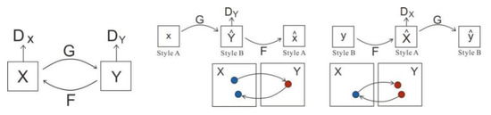
Figure 1.
Structure diagram of cyclic consistency generative adversarial network [27]. Model contains the two mapping functions and , and the associated adversarial discriminators and . encourages to translate into outputs indistinguishable from the domain , and vice versa for and . We introduced two cycle-consistency losses that illustrated the idea of translating from one domain to the other and back. We should arrive at where we started: forward cycle-consistency loss: , and backward cycle-consistency loss: .
The loss included antagonism and cyclic consistency loss . The former ensured that the generator and discriminator mutually evolved to produce more realistic images; the latter that the input and output images had the same content but different styles, because images must be converted between source and target domains. The antagonism is
During the mapping from X to Y, stands for generator and tries to generate an image that looks similar to the image in the target domain Y, and distinguishes the generated image from the real image . is the probability that the discriminator recognized the true data as true data; and is the probability that the discriminator still recognized the false data generated by the generator as false data. The adversarial loss is the sum of the two. The cyclic consistency loss is
where and are two image domains, is the generator of close samples; and refers to the generator of close samples. When we fed into , we got a fake graph called . Then we fed into to get an even faker graph called . This constituted a cycle. was the generated mapped back to X, and was defined similarly.
2.1.2. U-GAT-IT
Based on CycleGAN, U-GAT-IT [28] adds an adaptive instance (AdaIN) regularization layer to control the style transfer process for image-to-image translation. As shown in Figure 2, the generator carries out image downsampling on the input terminal and combines it with residual blocks to enhance image feature extraction. The attention module is guided by AdaIN to obtain the transformed image by upsampling the residual block. The discriminator converts the decoding process into an authentication output.
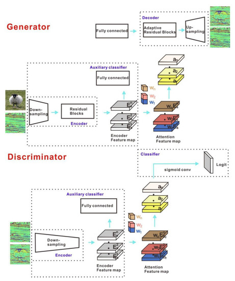
Figure 2.
Network structure of normalized unsupervised generation of adaptive layer instances [28]. The generator has a decoder module implemented by the AdaLIN algorithm more than in the discriminator. The input image of the generator creates the feature map through the encoding stage of the Encoder, and then an auxiliary classifier is added. The attention mechanism is introduced to maximize the pooling of the feature map. The prediction of a node is output through the full connection layer, and then the parameters of the full connection layer and the feature map are multiplied to obtain the feature map of attention. Finally, the output image is obtained through Decoder module . The discriminator compresses the input image at a deeper level and adds an auxiliary classifier . Finally, the output is judged by the classifier .
The model’s objectives include four loss functions, including antagonistic loss, which are used to match the generated and target image distributions:
In the mapping process from source domain to target domain , refers to the false data generated from source domain . The probability that the discriminator will still determine the false data generated by the generator in the source domain as false data is given by . is the probability that the discriminator will determine the true data as true data, and the adversarial loss is the sum of the two. Cyclic consistency loss reduced the mapping path from the source to the target domain. Given an image x ∈ , after the sequential translations of x from to and from to , the image should be successfully translated back to the original domain:
where refers to the false data generated from the source domain . We fed into to get the false data , which ideally should be comparable to the . This constitutes a cycle. We applied an identity consistency constraint to the generator to preserve the consistency of the color composition of the input and output images. Given an image x ∈, after the translation of x using , the image should not change:
Class activation map (CAM) loss is the biggest difference between the source and target domain. The auxiliary classifiers and help the generator and discriminator to evolve. For an image x ∈ {, }, and realize what makes the most difference between the two domains in the current state:
refers to the CAM loss of the generator in the source domain. If x is the true data, the cross-entropy output is ; if x is the false generated data, the cross-entropy output is . In order to make the generator as false as possible, should be as small as possible. The higher the discriminator’s ability to judge true data and false data, the better. refers to the probability that the auxiliary classifier collaborated with the discriminator to judge true data as true data as true data, and refers to the probability that the auxiliary classifier collaborated with the discriminator to continue to judge false data from the generator in the source domain as false data. The sum of the two, , is the CAM loss in the discriminator from the source domain to the target domain.
2.1.3. Lapstyle
Lapstyle [29] transmits a low-resolution global style mode through a drafting network, revises local details with high resolution through a correction network, and generates image residuals according to the image texture and sketch extracted by a Laplace filter. Higher-resolution details can easily be generated by superimposing revision networks with multiple levels of the Laplacian pyramid. All pyramid-level output is aggregated to obtain the final stylized image, as shown in Figure 3.
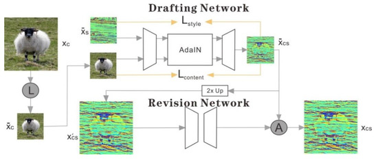
Figure 3.
Network structure of Laplacian pyramid network [29]. Firstly, the content image is reduced by two times, and , and in the image separately represent Laplacian concatenation and aggregation operations. At this time, the predefined style image is also reduced by two times to a low resolution version . In the drafting network stage, the content image and the style image after double down-sampling are generated through a encoder-decoder AdaIN module to generate a global but not detailed stylized image . In the revision stage of the network, twice the up-sampling processing and connecting with the residual detail image as the input, the stylized residual detail image is generated through a encoder-decoder module. Finally, we aggregate the two-level image pyramid and output the final stylized image .
The drafting network includes an encoder, several AdaIN modules and a decoder, as shown in Figure 4. The visual geometry group (VGG) encoder extracts corresponding granularity features at layers 2_1, 3_1, and 4_1, feeds them into an AdaIN module for aggregation, and merges them by jumping connection layers.
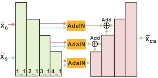
Figure 4.
Schematic diagram of drafting network [29]. After double down-sampling, the content image and the style image are extracted from the corresponding granularity features at the 1_1, 2_1, 3_1 and 4_1 layers. Then the features of the content and output of each layer of the AdaIN module are aggregated through an encoder–decoder AdaIN module. Finally, in each granularity of the decoder, the corresponding features are merged from the AdaIN module through the jump connection layer.
The revision network modified the rough stylized image by generating a residual detail graph of the image, and combined it with the rough stylized image to generate the final stylized image. As shown in Figure 5, the revision network has a simple, efficient codec architecture with only one undersampling and one upsampling layer. An image block discriminator helps the revision network capture fine block textures under adversarial learning.
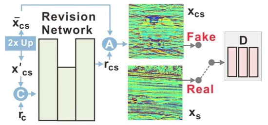
Figure 5.
Schematic diagram of network revision [29]. C and A represent concatenation and aggregation operations separately. The residual detail image is connected with the result image of the drafting network stage after double up-sampling. After revising the network, the residual detail image of the image is generated to modify the rough stylized image . Then is combined with the rough stylized image to generate the final stylized image which is output through the discriminator with the style image .
During training, the drafting and revision networks optimized the content and style, and the revision network adopted the adversarial loss function. We described the style and content loss and introduced the goals of each network. The Laplacian pyramid network is a single style for a single model during training, keeping one and one set of from the content set .
Following the STROTSS method, the rEMD and the commonly used mean-variance loss functions were combined into a style loss function. Given an image, we used the advance training VGG-19 encoder to extract a set of characteristic vectors for . The rEMD loss function measured the distance between the characteristic distribution of stylized images and . where denoted the distance of fitting the style map with pixels of the image and of the image. A smaller cosine distance term means that and are more similar. Assuming that and to be the properties of and , respectively, their rEMD losses are calculated as
The content loss function is adopted between and using normalized perceived loss and self-similarity loss. was equal to , and was equal to , because and had the same resolution. Perceptual loss is defined as
where represents the normalized channel direction . The purpose of self-similar loss is to maintain the relative relationship between the content and stylized images and is defined as
where and are the terms of self-similar matrices and , respectively. Here, is the cosine similarity .
In the training stage of the revision network, the parameters of the drafting network were fixed and the training loss was based on . To better learn local fine grain textures, a discriminator was introduced, and a revision network with an antagonistic loss term was trained. The overall loss function is defined as
where denotes the revision network, denotes the discriminator, and β controls the balance between basic style transfer loss and antagonism loss. is the basic content loss, and is the standard adversarial training loss.
2.2. Seismic Dataset Preparation
Herein, we discuss the required data, including seismic data, from a work area and the open-source COCO image instance segmentation dataset. The seismic profile classification dataset, shown in Figure 6, contains only seismic profiles and no artificial interpretations to avoid data leakage. These seismic profiles were selected because the faults were less developed, and the alignment of the in-phase axis was clear, thus avoiding ambiguity from the influence of geological structures or data processing. This avoided the influence of faults in the seismic profile classification dataset on the training of the Laplacian pyramid network. The seismic section classification dataset was only used in the image style migration network. We did not need to mark it, as it only provided the unique type, i.e., the seismic data class, used to pre-train the classification network in the style migration network, which this time was used to transfer the global style and local texture of the seismic section. Therefore, after migration, the image only had the sequence texture features of seismic data, and there were no obvious fault features to influence subsequent modeling.
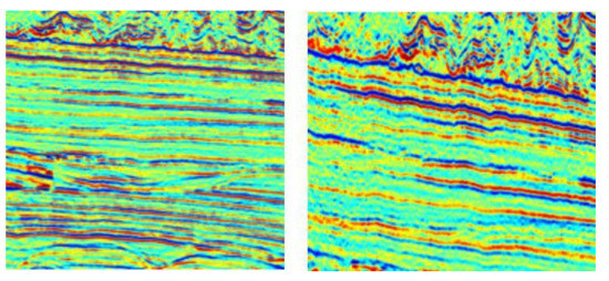
Figure 6.
Image of seismic profile classification dataset.
Microsoft Common Objects in Context (MS COCO) is a large, rich, object detection, segmentation, and subtitled dataset that takes scene understanding as the target and is mainly extracted from complex daily scenes. The target in the image is calibrated by precise instance annotation. The dataset includes 91 categories of objects, 328,000 images, and 2.5 million labels. So far, the largest dataset with semantic segmentation has 80 categories and more than 330,000 images of which 200,000 are labeled. Some images are shown in Figure 7.

Figure 7.
Images from COCO dataset.
3. Results
This section focuses on how the three models CycelGAN, U-GAT-IT, and Lapstyle are network trained in seismic image profile stylization. We compared and analyzed the results after stylized mapping both subjectively and objectively and use them to evaluate the quality of the stylized images.
3.1. Network Training of Each Algorithm
In the experiments, CycleGAN and U-GAT-IT were trained on 256 pixels with the parameter batch size set to 1. The Lapstyle experiment had three stages: the drafting network trained on 128 pixels, the revision network trained on 256 pixels with a batch size of 14 and the revision network trained on 512 pixels, with a batch size of 5.
The training results of the drafting network are shown in Figure 8, from which it can be seen that the content and style of the resulting graph were retained globally under the premise of migrating the profile style, so the Lapstyle experiment could be continued.
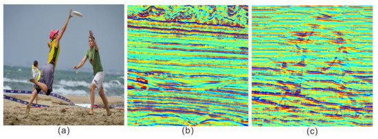
Figure 8.
Drafting network training results. Transferring the global pattern at low resolution, the result image has only a fuzzy contour; the leg and other details are seriously lost; and the overall color is dark. (a) Content; (b) Style; (c) Drafting network training transfer of the overall style of the graph (b) while ensuring that the content of the graph (a) as far as possible was not lost.
In the second stage of the experiment, the training weight of the drafting network was added. Five groups of control experiments were set according to the proportional relationship between content and style weights. The style weight was 3.0, 2.0, 1.0, 1.0, 1.0, with corresponding content weights of 1.0, 1.0, 1.0, 2.0, 3.0, as shown in Figure 9.
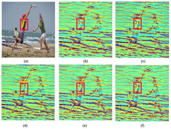
Figure 9.
First training results of revision network. (a) Content. (b) Content weight = 1.0; style weight = 3.0; and the woman’s clothing contour is fuzzy. (c) Content weight = 1.0; style weight = 2.0; seismic profile is obviously stylized; and the woman’s clothing details are not prominent. (d) Content weight = 1.0; style weight = 1.0; and the contour is clear, but the color is not obvious. (e) Content weight = 2.0; style weight = 1.0; the woman’s clothing is similar in color to (a) and more prominent. (f) Content weight = 3.0; style weight = 1.0; and the effect is equivalent to (e).
Figure 9 shows the top part of a woman framed by a red box. From left to right, the shape of the top becomes gradually clearer and the color more prominent. The effect of (f) is similar to that of (e), but in principle the greater the degree of style change the better because the image content can be recognized by the naked eye. Therefore, the migration effect of content weight 2 and style weight 1 was the best for the first modified network training. The training weight was assigned to the second modified network training, and five groups of control experiments were set. Figure 10 shows a woman’s calf framed by a red box. In (c), the outline of the leg is not clear, while in (d), the details of the calf muscle can clearly be seen. Based on the above principles, the migration effect of content weight 1 and style weight 1 were the best in the second revision of network training.
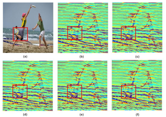
Figure 10.
Second training results of revision network. Visually, the overall color is brighter than before, and the beach position, shape of the waves and details of the woman’s legs are further highlighted. (a) Content. (b) Content weight = 1.0; style weight = 3.0; the woman’s leg muscle contour is blurred. (c) Content weight = 1.0; style weight = 2.0; the woman’s leg detail lines are too thick to finely restore the original leg features. (d) Content weight = 1.0; style weight = 1.0; the contour is clear and the overall composition is bright. (e) Content weight = 2.0; style weight = 1.0; the effect is equivalent to (d). (f) Content weight = 3.0; style weight = 1.0; the effect is equivalent to (e).
Some of the experimental results are shown in Figure 11, where several representative images were selected to facilitate the comparison of the experimental results. On the whole, it can be seen that the image changed; however, the original content information style of the migrated images changed fundamentally, and their characteristics and backgrounds showed features of the in-phase axis of the seismic section. Figure 11c shows that all seismic profile styles were transferred at low resolution. The image is blurry, and the color of the image content is almost covered by that of the style image. Therefore, modification was carried out, and residual texture details were extracted at high resolution. In Figure 11d, on the basis of the successful migration of the seismic profile style, the color of the woman’s clothes in the beach figure is differentiated; the motorcycle figure is clearly outlined; and the letters in the stamp figure can be identified. The variety and quality of textures in Figure 11e are significantly improved, and the stylistic characteristics of the seismic sections were obtained while preserving the content. The image is clearer, and the overall artistic effect of the visual image has been improved.
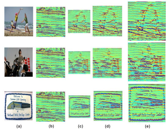
Figure 11.
Experimental results. All the content and style images were observed by our network training. (a) Content. (b) Style. (c) Drafting network training results. (d) First training results of revision network: content weight = 2.0 and style weight = 1.0. (e) Second training results of revision network” content weight = 1.0 and style weight = 1.0.
Figure 12 shows changes in the mean value of the generator and discriminator loss functions in the training of each network with the MS-COCO dataset transformed by the seismic profile style. Iter is the number of iterations, The Lapstyle and U-GAT-IT algorithms recorded every 3000 steps, and trained 30,000 pieces of data in total. The CycleGAN network generation model was limited by a rate of only 6000 iterations. During the training, the loss function values of CycleGAN, U-GAT-IT and Lapstyle all oscillated within an acceptable range; the convergence was general, and the obtained style transfer model was stable.
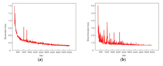
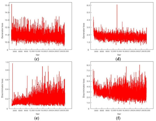
Figure 12.
Training loss comparison of each network. The smaller the probability that false data were judged as false by the discriminator, the better the probability that the false data generated by the generator tended to real data. The two fought against each other and finally maintained a relatively stable range. (a) During CycleGAN network training, the number of iterations was 6000; the generator loss decreased significantly; and tended to be stable with the increase in iterations. (b) During CycleGAN network training, the number of iterations was 6000, and the loss in the discriminator decreased with the increase in the number of iterations and finally oscillated in a stable range. (c) During U-GAT-IT network training, the number of iterations was 30,000 and the generator loss oscillated in a stable range of 10–14. (d) During U-GAT-IT network training, the number of iterations was 30,000 and the loss in the discriminator oscillated in a stable range of 1–3. (e) In the process of Lapstyle network training, the number of iterations was 30,000 and the generator loss fluctuated in a stable range of 0–0.6. (f) During Lapstyle network training, the number of iterations was 30,000 and the generator loss oscillated in a stable range of 1–6.
3.2. Comparative Analysis of Results
We selected CycleGAN, U-GAT-IT, and Lapstyle for comparative experiments, using the VGG-19 model for network training. The selected target content images were from the COCO dataset, and the style images were from the Yinggehai seismic profile dataset.
Figure 13 shows the effect of the abovementioned style transfer method, and a comparison of the experimental results of sheep, beach, and food. The subjective visual effects of CycleGAN’s experimental results showed that the original content image color was completely covered, and the stylized image lost part of the original content color information, resulting in ambiguity. U-GAT-IT improved upon CycleGAN, and the quality of the generated image obviously improved. In contrast, the stylized images drawn by the Lapstyle method were transformed from the real world into the seismic profile style based on the premise that the original content color and detail information were not lost, and both the overall contour migration and texture detail processing significantly improved.
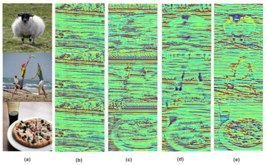
Figure 13.
Comparison of experimental results. (a) Content; (b) Style; (c) The style transfer graph generated by CycleGAN model has serious content information loss. (d) The style transfer graph generated by U-GAT-IT model has serious content information loss and dark overall image color. (e) The content information of the style transfer graph generated by Lapstyle model is well preserved and the color is relatively prominent.
4. Discussion
It was necessary to evaluate the stylized image quality both subjectively and objectively. Visual observation showed that the Lapstyle style transfer effect was obviously better than that of the other two methods, but there was no unified index for objective evaluation. Therefore, we adopted the widely recognized Structure Similarity Index Measure (SSIM) and an image fusion quality evaluation index called [30] to evaluate the quality of the stylized images objectively, and use the running time of an algorithm to evaluate the efficiency of the migration method.
The SSIM measures the similarity of image structures in brightness, contrast, and structure. uses local metrics to estimate the performance of input style and content images in the fused image. A higher indicates a fused image of better quality.
Figure 14 shows the SSIM, , and running time of stylized images generated by CycleGAN, U-GAT-IT, and Lapstyle. Compared with CycleGAN and U-GAT-IT, the stylized drawn image from Lapstyle had a higher fusion quality and greater structural similarity to the original image, indicating that its color information had been retained as much as possible and been transformed to the seismic profile style, which has the texture characteristics of the in-phase axis. The average running time of Lapstyle was 6.15 s, which was better than that of CycleGAN or U-GAT-IT (12.20 s and 20.21 s, respectively). Lapstyle also showed a better overall visual effect.
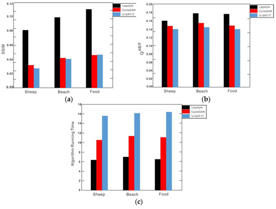
Figure 14.
Evaluations of statistical indicators. (a) Taking the sheep, beach and food images as examples, the SSIM evaluated the quality of stylized images: the higher the SSIM index, the better the quality of the stylized image. The SSIM index of Lapstyle was significantly higher than for CycleGAN or U-GAT-IT. (b) Taking the sheep, beach and food images as examples, was used to evaluate the quality of stylized images: the higher the index, the better the quality of the stylized images. Lapstyle’s index was slightly higher than that of CycleGAN or U-GAT-IT. (c) Taking the sheep, beach and food images as examples, the running time of the algorithm was used to evaluate the efficiency of the migration method. Lapstyle generated the style migration effect map with the fastest speed and in the shortest time.
The COCO dataset was uniform in format, rich in content and variety, and suitable for training convolutional neural networks. The results of the seismic profiling style conversion based on the COCO dataset showed that features such as overall contour information and texture detail can be preserved better based on the selection of a suitable migration algorithm. Because the style migration method was based on the computer field of vision, it had a strong similarity to most of the fault interpretations carried out by seismic profiling. Similarly, this method is applicable to the interpretation of special geological phenomena, such as seismic facies or diapir identification, which are visually identified. After the style transfer of the COCO dataset was completed, the semantic segmentation model was trained for the COCO dataset with a stylized seismic profile. The training label maintained the label of the original COCO dataset. After training was completed, the front weight of the semantic segmentation model was frozen, and only the last two weights were retained as the training state. The model structure of the last two layers was modified, and the number of channels in the last layer was changed from 81 to 2. Next, the dataset was replaced by the fault dataset of the target work area from the stylized COCO dataset to reduce the learning rate and to retrain, meaning that only the weights of the last two layers were fine-tuned. After the loss value converged, the fault recognition model of the target work area based on the stylized COCO dataset was obtained. This method solved the problem of insufficient training samples of actual seismic data and provided a feasible solution that could expand the application of artificial intelligence methods in interpreting seismic data.
5. Conclusions
In this paper, we addressed the lack of sufficient training samples for artificial intelligence methods in seismic data interpretation applications, and proposed the use of style migration to convert the image recognition COCO dataset into a seismic profile format. We drew three main conclusions.
- Using a suitable style migration algorithm, the COCO dataset was well migrated into the seismic profile format, which retained the overall contour information and features such as texture details more completely. This result can be used to increase artificial intelligence seismic interpretation training samples and realize the application of artificial intelligence to visually discernable seismic geological interpretation tasks such as fault interpretation, seismic facies interpretation, and special morphological geological body interpretation.
- By comparing the effects of multiple style migration models, the Laplace pyramid network was preferred for carrying out seismic profile stylization research. It transmitted low-resolution global style patterns through the drafting network, corrected high-resolution local details through the correction network, and aggregated all pyramid layers to output a final stylized seismic profile image. Experiments showed that this method ensured that the overall style pattern was effectively transmitted without losing the original image content. It provided theoretical guidance for fast and objective application of the model to learn seismic data features.
- The quality of stylized images was objectively evaluated on two indexes, SSIM and and the efficiency of the migration method was evaluated for algorithm running time. Thus, a quantitative evaluation of the good or bad quality of stylized images was achieved.
However, this study was limited to an analysis of the effect of stylized conversion, so further work and discussion are needed before implementing artificial intelligence algorithms combined with the training set of actual seismic interpretation data.
Author Contributions
Conceptualization, H.H. and R.S.; methodology, W.L.; software, W.L.; validation, H.H., W.L. and R.S.; formal analysis, H.H.; investigation, W.L.; resources, R.S.; data curation, W.L.; writing—original draft preparation, W.L.; writing—review and editing, H.H.; visualization, C.R.; supervision, J.Z.; project administration, R.S.; funding acquisition, H.H. All authors have read and agreed to the published version of the manuscript.
Funding
This work was supported by the National Natural Science Foundation of China (No. 42002149), the Natural Science Foundation of Heilongjiang Province (No. LH2021D007).
Acknowledgments
We thank all graduate research assistants who helped with data collection.
Conflicts of Interest
The authors declare no conflict of interest.
References
- Safaei-Farouji, M.; Kamali, M.R.; Rahimpour-Bonab, H.; Gentzis, T.; Liu, B.; Ostadhassan, M. Organic geochemistry, oil-source rock, and oil-oil correlation study in a major oilfield in the Middle East. J. Pet. Sci. Eng. 2021, 207, 109074. [Google Scholar] [CrossRef]
- Zhang, Z.; Chen, Z.; Yang, B. New understanding of Zhidan Group based on conventional seismic interpretation and inversion method. Coal Chem. Ind. 2021, 44, 67–70. [Google Scholar]
- Gersztenkorn, A.; Marfurt, K.J. Eigenstructure-based coherence computations as an aid to 3D structural and stratigraphic mapping. Geophysics 1999, 64, 1468–1479. [Google Scholar] [CrossRef]
- Marfurt, K.J.; Kirlin, R.L.; Farmer, S.L.; Bahorich, M.S. 3-D seismic attributes using a semblance-based coherency algorithm. Geophysics 1998, 63, 1150–1165. [Google Scholar] [CrossRef] [Green Version]
- Sun, X.; Du, S. The research of coherence technique algorithm and its application in seismic data interpretation. J. Pet. Univ. Nat. Sci. Ed. 2003, 27, 32–35. [Google Scholar]
- Cai, H. Improved algorithm of variance volume and its application in seismic interpretation. Coalf. Geol. Explor. 2008, 1, 74–76. [Google Scholar]
- Wang, J.; Wang, R. Fault identification method based on variance coherence. J. Eng. Geophys. 2006, 13, 46–51. [Google Scholar]
- Dorigo, M.; Gambardella, L.M. Ant colony system: A cooperative learning approach to the traveling salesman problem. IEEE Trans. Evol. Comput. 1999, 1, 53–66. [Google Scholar] [CrossRef] [Green Version]
- Middendorf, M.; Reischle, F.; Schmeck, H. Multi colony ant algorithms. J. Heuristics 2002, 8, 305–320. [Google Scholar] [CrossRef]
- He, H.; Wang, Q.; Cheng, H. Application of multi-scale edge detection technique in low-order fault identification. J. Pet. Nat. Gas 2010, 32, 226–228. [Google Scholar]
- Song, J.; Sun, Y.; Ren, D. Structure-oriented gradient attribute edge detection technique. Geophys. J. 2013, 56, 3561–3571. [Google Scholar]
- Wu, X.; Fomel, S. Automatic fault interpretation with optimal surface voting. Geophysics 2018, 83, 67–82. [Google Scholar] [CrossRef]
- Liu, Z.J.; He, X.L.; Zhang, Z.H. Fault identification technique based on 3D U-NET full convolutional neural network. Prog. Geophys. 2021, 36, 2519–2530. [Google Scholar]
- Badrinarayanan, V.; Kendall, A.; Cipolla, R. Segnet: A deep convolutional encoder-decoder architecture for scene segmentation. IEEE Trans. Pattern Anal. Mach. Intell. 2017, 39, 2481–2495. [Google Scholar] [CrossRef]
- Chehrazi, A.; Rahimpour-Bonab, H.; Rezaee, M.R. Seismic data conditioning and neural network-based attribute selection for enhanced fault detection. Pet. Geosci. 2013, 19, 169–183. [Google Scholar] [CrossRef]
- Wu, J.; Liu, B.; Zhang, H.; He, S.; Yang, Q. Fault Detection Based on Fully Convolutional Networks (FCN). J. Mar. Sci. Eng. 2021, 9, 259. [Google Scholar] [CrossRef]
- Wu, X.M.; Shi, Y.Z.; Fomel, S. Convolutional neural networks for fault interpretation in seismic images. In Proceedings of the 2018 SEG International Exposition and Annual Meeting, Anaheim, CA, USA, 14–19 October 2018. [Google Scholar]
- Yang, J.; Ding, R.W.; Lin, N.T. Research progress of intelligent identification of seismic faults based on deep learning. Prog. Geophys. 2022, 37, 298–311. [Google Scholar]
- Wu, X.; Geng, Z.; Shi, Y. Building realistic structure models to train convolutional neural networks for seismic structural interpretation. Geophysics 2019, 85, WA27–WA39. [Google Scholar] [CrossRef]
- Liu, Z.; Yang, X.; Gao, R.; Liu, S. Remove Appearance Shift for Ultrasound Image Segmentation via Fast and Universal Style Transfer. In Proceedings of the 2020 IEEE 17th International Symposium on Biomedical Imaging (ISBI), Iowa City, IA, USA, 3–7 April 2020. [Google Scholar]
- Qu, Y.Y.; Chen, Y.Z.; Huang, J.Y. Enhanced Pix2pix Dehazing Network. In Proceedings of the 2019 IEEE/CVF Conference on Computer Vision and Pattern Recognition (CVPR), Long Beach, CA, USA, 15–20 June 2019; 8160–8168. [Google Scholar]
- Yin, X.; Zhong, P.; Xue, W.; Xiao, Z.; Li, G. Uav image target detection method under foggy weather conditions by style transfer. Aviat. Weapon 2021, 28, 22–30. [Google Scholar]
- Chen, S.; Hai, X.; Yang, X.; Li, X. SAR and optical image registration algorithm based on style transfer invariant feature. Syst. Eng. Electron. 2021, 44, 1536–1542. [Google Scholar]
- Cao, K.; Jing, L.; Lu, Y. CariGANs: Unpaired photo-tocaricature translation. ACM Trans. Graph. 2018, 37, 1–14. [Google Scholar]
- Peśko, M.; Svystun, A.; Andruszkiewicz, P. Comixify: Transform video into comics. Fundam. Inform. 2019, 168, 311–333. [Google Scholar] [CrossRef] [Green Version]
- Wang, T.; Deng, L.J. A method to realize the special effect of fluid style (vortex) Van Gogh oil painting. Inf. Commun. 2014, 7, 38–40. [Google Scholar]
- Zhu, J.Y.; Park, T.; Isola, P. Unpaired image-to-image translation using cycle-consistent adversarial networks. In Proceedings of the 2017 IEEE International Conference on Computer Vision (ICCV), Venice, Italy, 22–29 October 2017; pp. 2242–2251. [Google Scholar]
- Kim, J.; Kim, M.; Kang, H. U-GAT-IT: Unsupervised Generative Attentional Networks with Adaptive Layer-Instance Normalization for Image-to-Image Translation. In Proceedings of the 2020 International Conference on Learning Representations (ICLR), Addis Ababa, Ethiopia, 25–30 April 2020. [Google Scholar]
- Lin, T.; Ma, Z. Drafting and Revision: Laplacian Pyramid Network for Fast High-Quality Artistic Style Transfer. In Proceedings of the 2021 IEEE/CVF Conference on Computer Vision and Pattern Recognition (CVPR), Nashville, TN, USA, 20–25 June 2021. [Google Scholar]
- Bondzulic, B.; Petrovic, V. Objective image fusion performance measure. Mil. Tech. Cour. 2020, 52, 181–193. [Google Scholar] [CrossRef] [Green Version]
Publisher’s Note: MDPI stays neutral with regard to jurisdictional claims in published maps and institutional affiliations. |
© 2022 by the authors. Licensee MDPI, Basel, Switzerland. This article is an open access article distributed under the terms and conditions of the Creative Commons Attribution (CC BY) license (https://creativecommons.org/licenses/by/4.0/).