Machine Learning in Solar Plants Inspection Automation

Abstract

The emergence of large photovoltaic farms poses a new challenge for quick and economic diagnostics of such installations. This article presents this issue starting from a quantitative analysis of the impact of panel defects, faulty installation, and lack of farm maintenance on electricity production. We propose a low-cost and efficient method for photovoltaic (PV) plant quality surveillance that combines technologies such as an unmanned aerial vehicle (UAV), thermal imaging, and machine learning so that systematic inspection of a PV farm can be performed frequently. Most emphasis is placed on using deep neural networks to analyze thermographic images. We show how the use of the YOLO network makes it possible to develop a tool that performs the analysis of the image material already during the flyby.

1. Introduction

The rapid growth of the capacity to generate electricity from renewable technologies observed in recent years can be further accelerated by the challenges set by a recent political situation. Renewable capacity growth between 2021 and 2026 is expected to be 50% higher than between 2015 and 2020, driven by the greater government policy support and more ambitious clean energy targets [1]. Global renewable electricity capacity is projected to increase by more than 60% by 2026 compared to 2020 levels, equivalent to the current combined fossil fuel and nuclear capacity, reaching more than 4.8 GW. Renewable sources are expected to account for nearly 95% of global capacity growth by 2026. Solar photovoltaic (PV) installations alone are expected to contribute to more than half of that growth. In many countries, the general trend is to develop larger installations with power reaching several tens or even hundreds of megawatts.

Although it may seem strange, many PV farm operators show little concern in quickly detecting problems in the installation operation and even in immediately repairing the faults detected. This results from the economic balance sheet, which shows that the potential loss of profit due to the reduced energy production is lower than the costs of monitoring and repair [2] (pp. 60–62). However, even the authors of the mentioned report state that ignoring defects is not a viable solution in the long term. In the next section of this paper, we will report experiments showing that even a temporary deterioration of the operating conditions of a cell by only partial shading results in measurable losses which grow if the problem is more severe. This section is aimed to convince the reader that neglecting the problems of vegetation or partial failures of some modules can quickly lead to serious deterioration of the whole plant. Only systematic and precise detection and localization of defects in PV modules can ensure the proper service life and efficient production of electricity, and thus the reliable operation of entire installations at a reasonable cost [3,4].

Operators of larger photovoltaic plants face a new challenge in ensuring the proper operation of a facility that often exceeds 100 hectares. They have to answer the question of whether to invest sufficient resources for systematic inspection to detect problems such as module damage or malfunctions caused by vegetation growth or to accept lower plant efficiency. The problem of monitoring module quality also applies to small domestic installations. Although they are not significant in terms of territory, they are usually located in places that are difficult to access, and the budget allocated by the owner for servicing the installation is usually very limited. The work of Hong and Pula [5] is a broad overview and attempt to categorize methods for testing defects in PV modules, including different data acquisition methods: visual method, thermal method, and electrical method. The conventional methods of identification and localization of failures are based on electrical measurements [4] and can be theoretically used for remote supervision of the system. However, for a large farm, this approach requires a tremendous extension of the sensing and communication infrastructure. Thus, the quest for cheaper approaches is still ongoing.

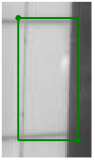
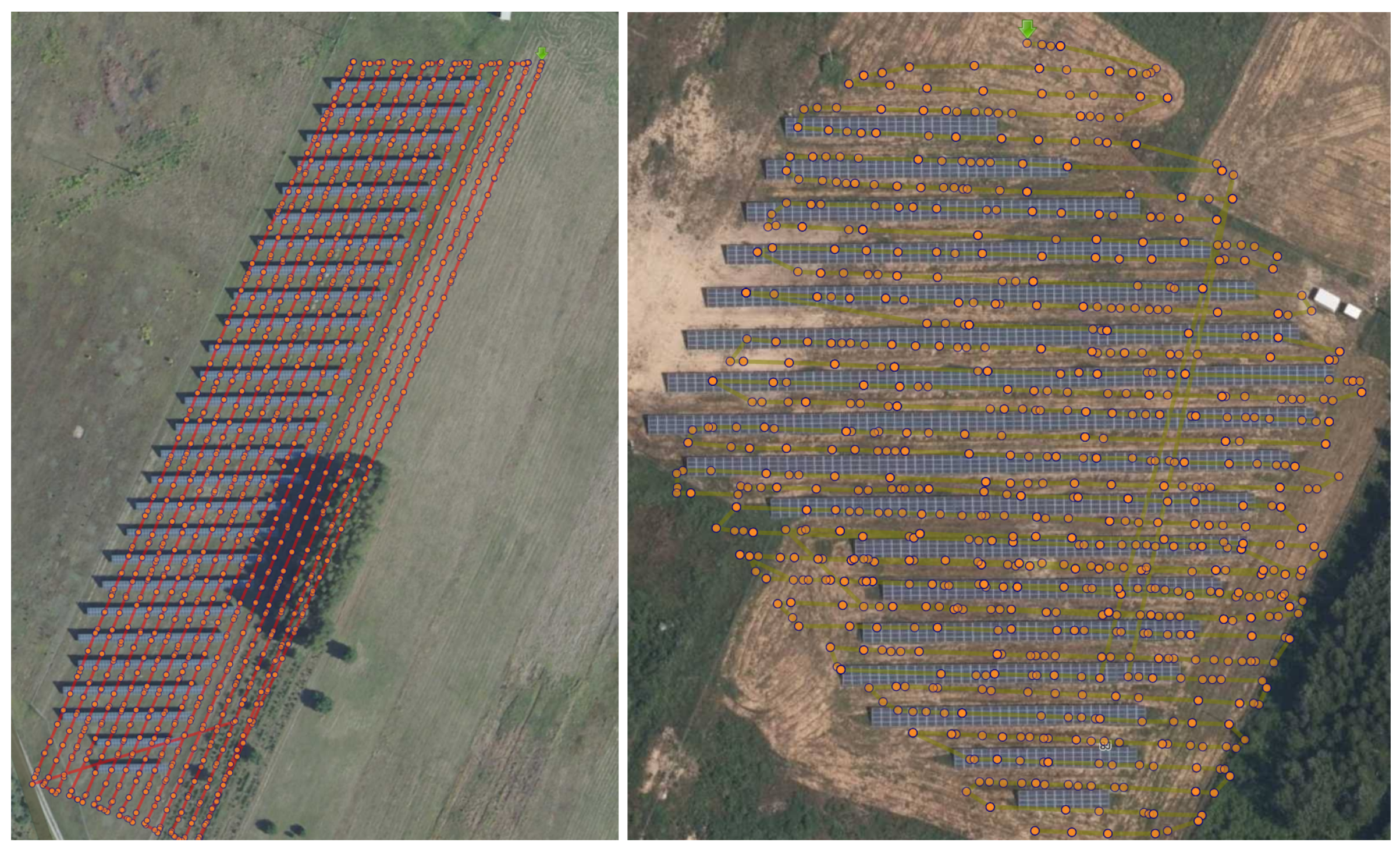
Malfunctions of a photovoltaic installation caused by faulty modules or electronic components or just shading of installation parts can be easily and quickly detected by analyzing images taken with a thermal imaging camera. In the case of installations that are difficult to access or extensive, such images are best taken with the help of an unmanned aerial vehicle (UAV) which can be controlled manually or appropriately programmed based on a map of the installation (see Figure 1). In the latter case, the flight over the farm is performed completely automatically based on GPS coordinates. Each image on top of the visible image and thermal data also contains a fairly precise location and information about the camera’s position, which allows locating the damage detected in the image on a map of the installation.

As a result of flying over a large farm, a considerable amount of photographic material is produced: the authors’ experience shows that per 1 MW there are 600–700 thermographic images (in resolution 640 × 512), and the total amount of data exceeds 5 GB (the camera usually also takes regular pictures in a higher resolution).

Flying over the farm and collecting the material is just the tip of the iceberg of the data processing task. If we rely on humans, it will take about 2 days of work for an experienced expert to review several hundred images and mark the detected problems. These estimates clearly show that without proper process automation, the diagnosis of a large farm would not be cheap.

Several methods have already been proposed to address this issue. While older works used human expertise [6] and digital signal processing [7,8,9,10,11] or parametric models of a PV module [12], the recent research trends tend to use a variety of machine learning tools such as traditional artificial neural networks [13,14,15] and support vector machines [16,17,18]. The introduction of deep neural networks has substantially changed the quality of automatic detection. Most recent works present applications of different deep (convolutional) neural networks (DNN or CNN) to the problem of automated evaluation of solar facilities. The actual review of almost 180 related papers can be found in [19]. The approaches are classified into two groups: algorithms based on digital image processing (DIP) and deep learning (DL) approaches. In both groups, we can find methods whose claimed accuracy reaches 100% [20,21]. However, according to the authors of this work, such results should be approached with great skepticism due to the huge variability of the data that such algorithms process. This variability is due to the different conditions under which the images can be taken, the variability of the equipment and its settings, and the qualifications of the UAV operator. Of course, we do not deny that the presented algorithms may achieve 100% accuracy on the data used in their preparation process (for example, deep learning). Still, this high accuracy on training data suggests that such an algorithm will achieve very good results when processing new data, as long as they are similar.

The goal of the authors is to develop a method that would provide high accuracy, defined as the ability to find more than 95 percent of defects, and at the same time would be fast enough to work in real time (meaning defects should be located on the fly) and could be used as both a desktop application and a web service. The second usage may be limited by the Internet connection quality at the controlled farm.

In this paper, an adaptation of You Only Look Once (YOLO) [22,23,24] deep convolutional neural network to automate the process of the detection and localization of the defects is discussed. The content is organized as follows: the next section briefly reviews selected problems that can occur in a photovoltaic system. The review focuses on presenting the measurable impact of a defect or incorrect installation on panel performance. It is then shown how these defects are visible in thermographic images, followed by a discussion of how to prepare the data used to train the CNN, which will be able to detect the defects. In the authors’ opinion, an appropriate dataset is currently the key to the successful application of CNNs. We will not describe the algorithm and methods used for object detection here. This work has already been conveyed elsewhere [23,25,26] and based on these reviews, the choice of one of the last versions of YOLO seems obvious. Nowadays, it is the fastest and yet most accurate DNN for object detection. However, the YOLO network was originally designed and trained on classical (visual) images, and adaptation to photovoltaic-oriented thermography requires additional data that are prepared and selected for this task. In the final section of this paper, we will show how the preparation of thermographic data affects the results of defect detection and classification. Four “recent” versions of the YOLO framework have been presented in the last three years [23,27,28,29]. We have chosen YOLOv4 here for two reasons. Firstly, it is the most mature yet sufficiently fast (the processing of a thermal image is an order faster than the preparation of this image from raw sensor data) and has reasonable accuracy (this accuracy is affected far stronger by the training dataset than by the YOLO version). It has been implemented in C++ and can be incorporated into the detection system as a dynamically loaded library, which seriously influences the system’s overall speed. The latest versions of YOLO are reported to run much faster, but the authors’ experience shows that the latest version of DNN software may not be as stable as the mature one. Considering that the last two versions were released in the last two months, we opted for the version we tested longer.

It has been shown [30] that carefully designed and properly trained DNN can model complex non-linear relationships. Since the beginning of the deep learning revolution, they have been successfully applied to problems of object detection [31,32,33]. In particular, the YOLO deep convolutional neural network was applied to detect defects in PV [34,35,36]. The novelty of this work lies firstly in using a newer version of YOLO (YOLOv4), which is considered better in terms of speed and accuracy, and secondly in a deeper analysis of the impact of data preparation on detection results.

2. Selected Problems of PV Installations

2.1. Technical Description of PV Modules

The correctness of the operation of the photovoltaic system is the main factor that primarily affects the efficiency and profitability of the investment and, consequently, the return-on-investment time, which should be as short as possible. One of the first systems to detect improper installation operating parameters is the inverter itself. Still, many faults are impossible to identify even by the inverter. The basic method of detecting module damage is to perform current–voltage characteristics, commonly known as the I–V curve. Based on it, it is possible to determine precisely what problems in the operation of a photovoltaic system are caused.

The typical I–V curve of a properly operating module is summarized in Table 1. Besides the characteristics, the important parameters of the module are:

• $P_{max}$—the maximal output power [W];
• $V_{mpp}$—output voltage at maximal power [V];
• $I_{mpp}$—current at maximal power [A];
• NOCT—standard temperature at nominal conditions [C];
• $\alpha$—temperature coefficient of $I_{sc}$ [%];
• $\beta$—temperature coefficient of $V_{oc}$ [%];
• $\gamma$—temperature coefficient of power [%].

To standardize and enable the comparison of the PV modules’ performance, it was necessary to standardize the measurement conditions. It has been achieved by establishing the benchmark (laboratory) conditions for measuring the parameters of PV modules, the so-called Standard Test Conditions (STC): insolation (irradiance) of 1000 [W/m${}^2$], PV module temperature 25 °C, and air mas factor of 1.5. STC is an industrial standard.

Table 1. Typical current–voltage characteristics of a properly functioning PV module.

Name	Symbol	Unit	Value STC
Output power	P	[W]	370	375	380	385	390
Output voltage	$V_{mp}$	[V]	34.11	34.41	34.71	35.00	35.30
Output current	$I_{mp}$	[A]	10.85	10.90	10.95	11	11.05
Open circuit voltage	$V_{oc}$	[V]	41.85	42.15	42.50	42.79	43
Short-circuit current	$I_{sc}$	[A]	11.37	11.42	11.47	11.52	11.57
Performance		[%]	20.31	20.59	20.86	21.13	21.41

γ = −0.35 (%/°C), β = −0.29 (%/°C), α = +0.048 (%/°C).

Table 1. Typical current–voltage characteristics of a properly functioning PV module.

Name	Symbol	Unit	Value STC
Output power	P	[W]	370	375	380	385	390
Output voltage	$V_{mp}$	[V]	34.11	34.41	34.71	35.00	35.30
Output current	$I_{mp}$	[A]	10.85	10.90	10.95	11	11.05
Open circuit voltage	$V_{oc}$	[V]	41.85	42.15	42.50	42.79	43
Short-circuit current	$I_{sc}$	[A]	11.37	11.42	11.47	11.52	11.57
Performance		[%]	20.31	20.59	20.86	21.13	21.41

γ = −0.35 (%/°C), β = −0.29 (%/°C), α = +0.048 (%/°C).

2.2. Experimental Evaluation of the Impact of Problems on PV Module Operation

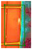
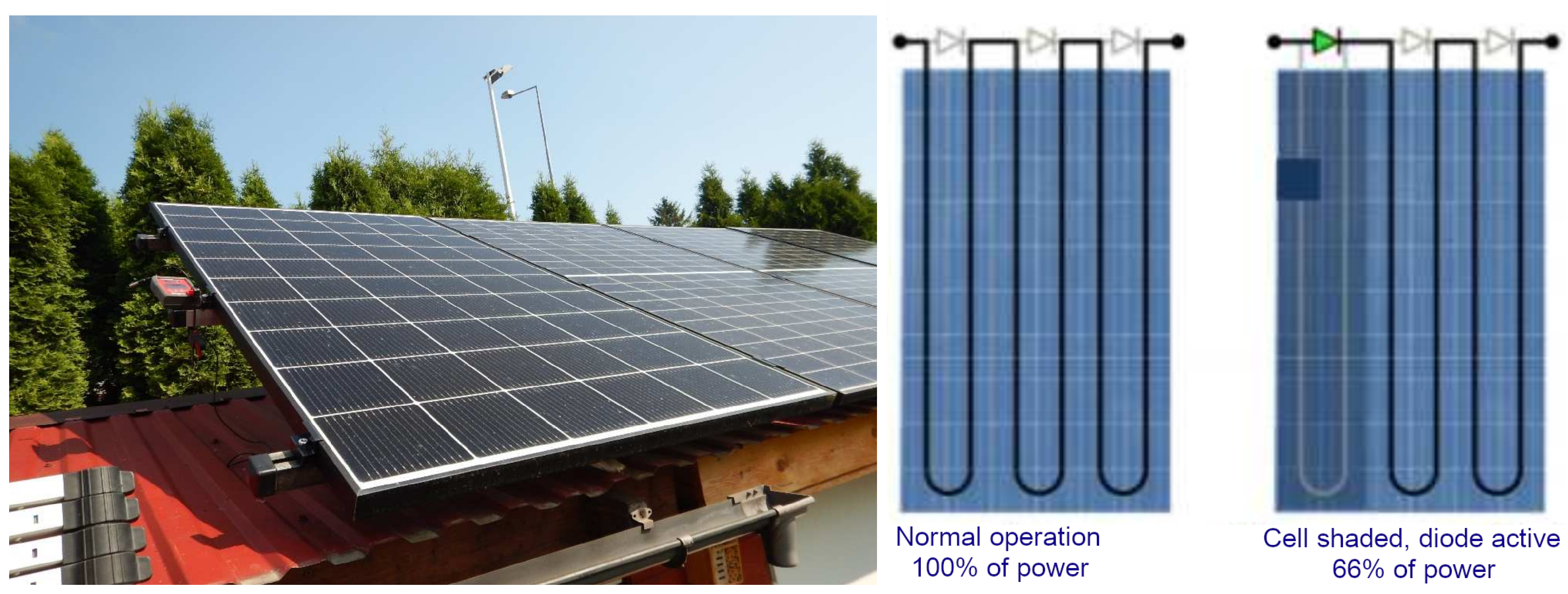
All measurements for this work were made on the existing photovoltaic system, shown in Figure 2. This system was designed and constructed with four photovoltaic modules of various models and types facing south and set at an angle of 35 degrees to the ground. The whole system is managed by a Hoymiles HM-1500 single-phase inverter. Thanks to this solution, it is possible to combine different photovoltaic modules into one system without worrying about the current–voltage mismatch. The system has been in operation for about two years now, thanks to which it is possible to observe a slight decrease in module efficiency associated with silicon cell degradation. The measurements took place in stable and cloudless weather at an air temperature oscillating around 30 C in the sun, with winds of negligible strength. To better illustrate the problems occurring during operation, one module was selected for the test—LG brand LG366N1C-N5, shown in the foreground of Figure 2. The PV module’s construction and orientation are shown on the right inset of Figure 2. The bypass diodes are located on the top of the module. This remark will be necessary when we begin to analyze the shading of a large part of the module. Plots of the nominal I–V curves are presented in Figure 3, Figure 4, Figure 5, Figure 6, Figure 7, Figure 8 and Figure 9.

The development of photovoltaics has been accompanied by the rapid development of the necessary diagnostic instruments. Most manufacturers of measurement equipment for the electrical industry offer devices for measuring photovoltaic installations. Companies such as Benning, Fluke, Metrel, HT Instruments, and Sonel have such instruments in their offerings. For this study, the Benning PV2 instrument was used along with the Benning Sun 2 attachment. In addition to the main measuring device, an important component of the system is the Sun2 attachment, whose most important functions are the measurement of sunlight intensity, air temperature, and PV module surface temperature. The attachment is equipped with an inclinometer for determining the angle of the PV module to the horizontal and a compass for determining the module’s azimuth. All these data are sent to the measurement module, where they are analyzed and included in the measurement results on an ongoing basis, presented graphically, and stored in the device’s memory.

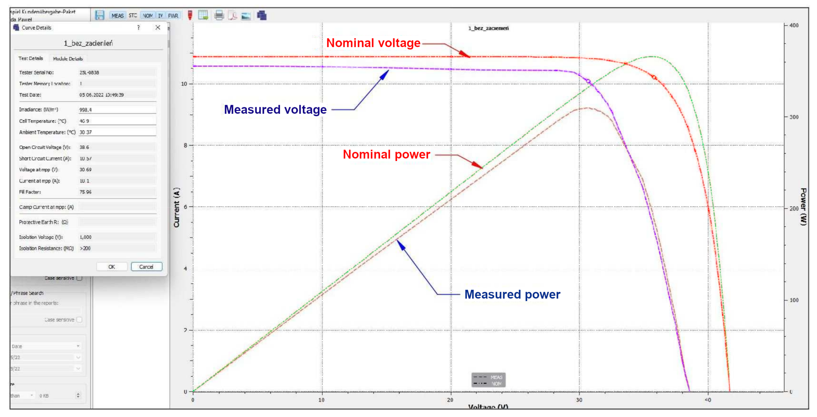
Figure 3 shows the current–voltage characteristics of a module illuminated correctly and without shading. However, it can be noted that the voltage and power values are different compared to nominal. This is due to several reasons [2]. The nominal characteristic is shown in a graph created for a new module operating under STC conditions; in the test case, we are dealing with a module that is already two years old and, therefore, partially degraded. An additional factor affecting the lower voltage operation is the high surface temperature of the module, which translates into a decrease in its voltage. The abovementioned factors are completely normal, and such modules are considered efficient.

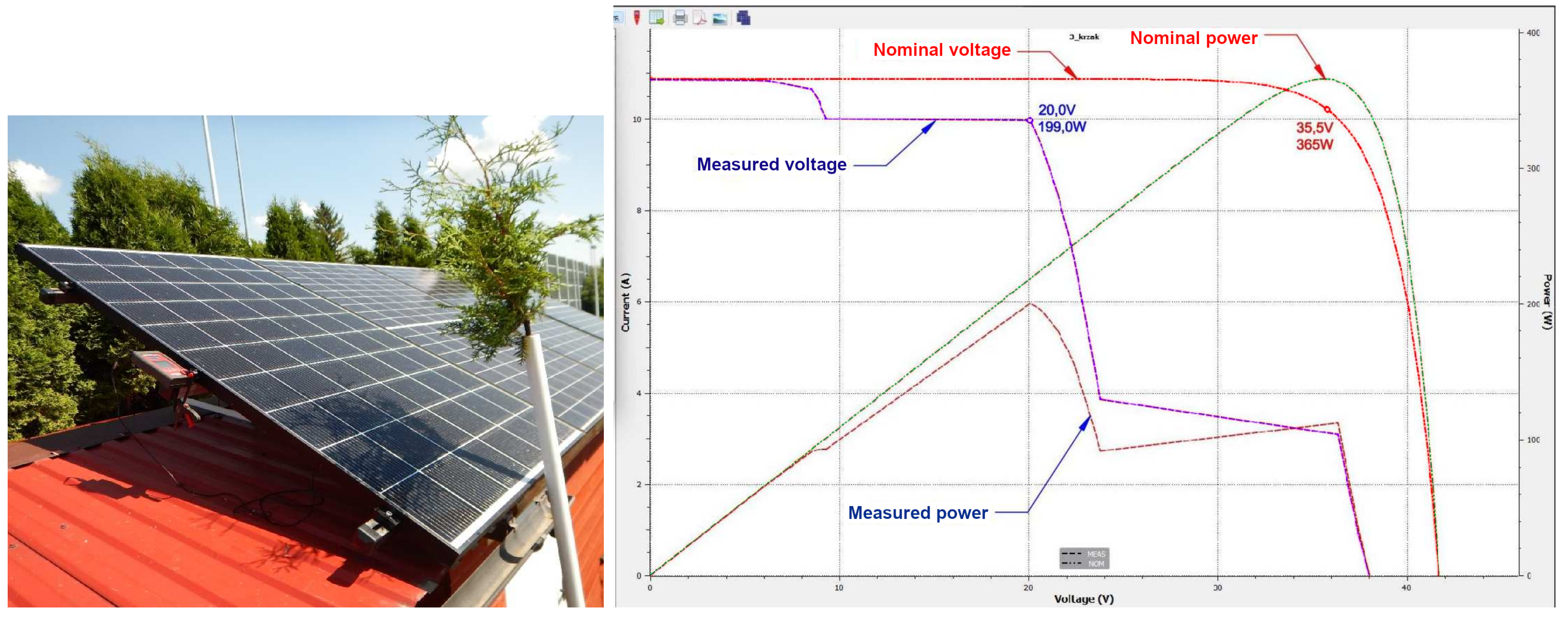
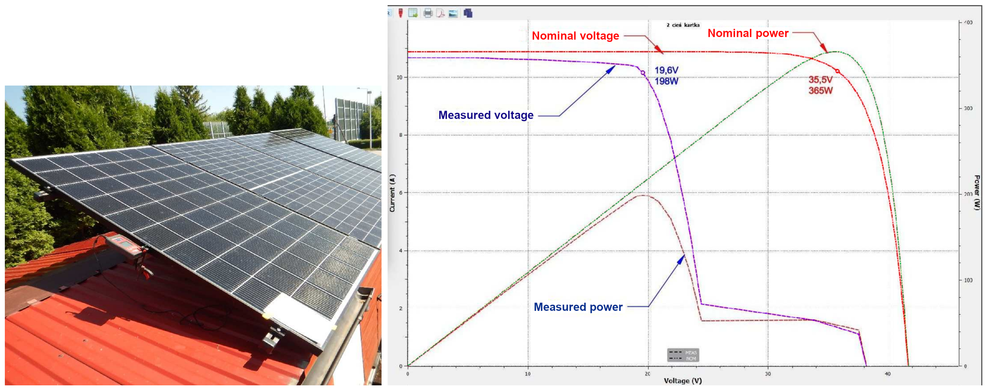
Figure 4 very clearly shows how the installation can be negatively affected even by a single relatively minor shading caused, for example, by a stuck leaf or accumulated bird droppings. The module’s power has dropped from a nominal value of 365 W to 198 W. To protect the module from the possible hotspot issue that is very dangerous in this case, bypass diodes are used, thus protecting the module and the entire installation from the possibility of damage to the module or even the occurrence of a fire. Comparing the nominal and measured power, we see the situation shown on the right inset of Figure 2.

Figure 5 presents the negative impact of shading by vegetation on system performance. This problem is often underestimated by owners of installations and can significantly affect the energy yield. In the case simulated above, the module’s power output dropped by more than 45% from 365 W to 199 W. In the case of a larger, not optimized system, consisting of a string of modules connected in series, losses of one module will translate proportionally into losses of the whole chain and thus will be very significant.

In the case of backyard installations, another concern is the impact of relatively small equipment mounted as standard on roofs on installation efficiency. Vent stacks, elements of antenna lashings, ladders, spires of lightning protection systems, etc., cause a phenomenon referred to in industry parlance as “traveling shadows” due to their movement with the sun’s path in the sky. An additional difficulty in assessing this type of shadow on a system is that its location changes depending on the year’s season and during the day. To eliminate the negative impact of the above devices on the PV system, it becomes necessary to use professional software that simulates shading areas on the system model. Only based on the analysis of such simulation results is it possible to determine how much negative impact on the system’s operation a particular device has so that an appropriate decision can be made. It may often be better to reduce the system by one module than place it in a shaded area, which will translate into a reduction in the efficiency of the entire installation.

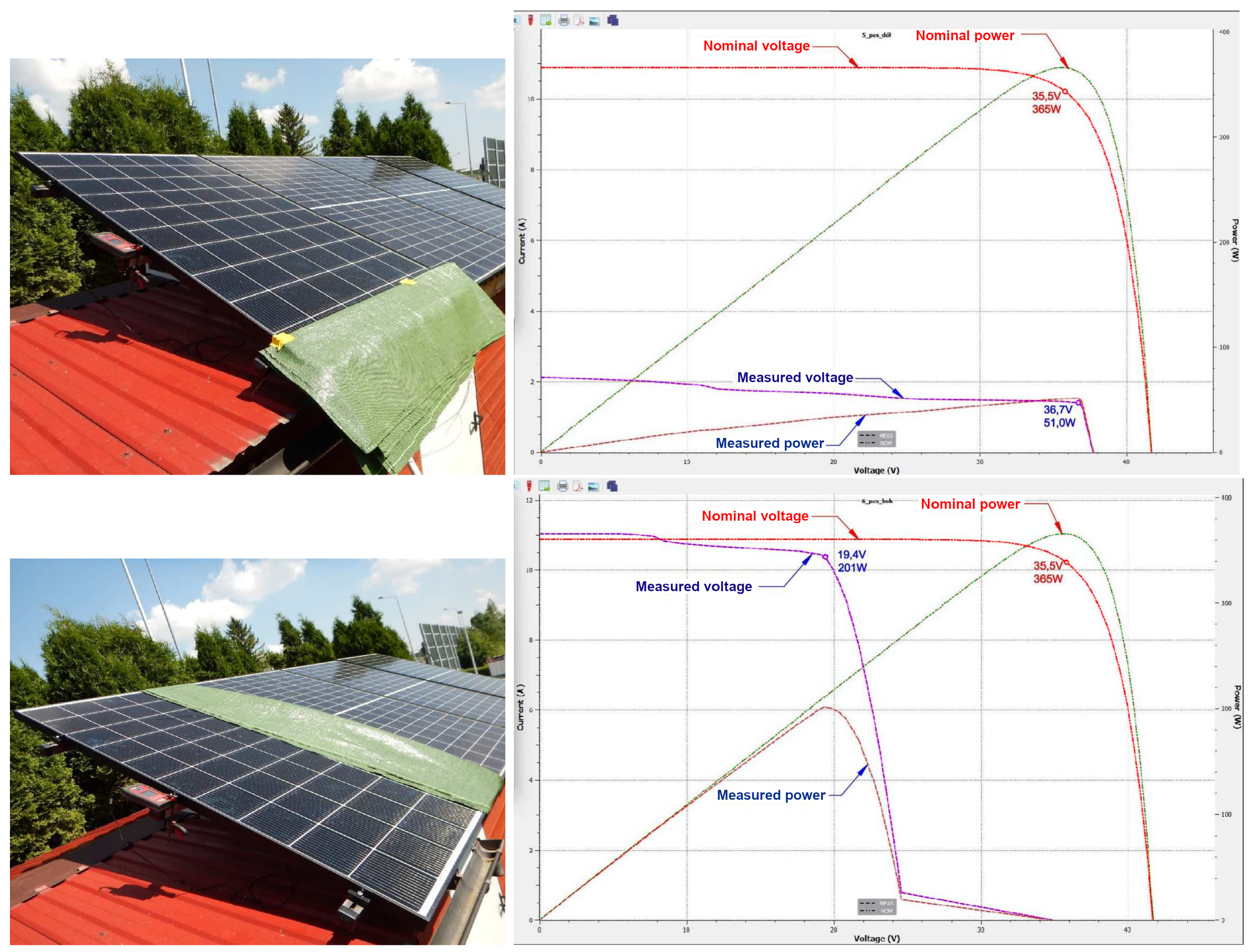
The top row of Figure 6 shows one of the worst possible shading cases. As can be seen on the I–V curve plot presented in the top-right inset Figure 6, covering the entire strip of cells in a module installed vertically, we can see a substantial loss of power: nearly 75%. In practice, such phenomena can occur in a case where sliding snow or a layer of dirt accumulates in the module’s lower part along its frame. This study tested traditional modules consisting of 60 cells to demonstrate the importance of the module’s correct orientation and inclination. Especially for small installations, horizontal mounting is a common mistake. With today’s 120-cell module (Half-Cut) technology, it is no longer as troublesome and loss-carrying as was the case with the older 60-cell modules.

In the top-left photograph in Figure 6, we see a 60-cell module, where green fabric obscured the lower strip of the module, covering one row of cells. Such a situation often occurs when dealing with sliding snow or vegetation (grass) growing along the lower edge of the panels installed near the ground. Obscured in this way, the module practically stops working altogether, all bypass diodes are activated, and the module’s generation drops to near zero.

The bottom row of Figure 6 shows the characteristics of the PV module shaded along the side edge. We can imagine that such a module is installed in a horizontal position. In such a case, if the sliding snow obscured its entire edge, only one bypass diode would operate, resulting in losses of 30–35%, which is far more favorable than vertical installation. As already mentioned, Half-Cut modules have significantly reduced the negative impact of obscuring the bottom edge of the cells on the operation of modules installed vertically. However, horizontal mounting is still far more advantageous and justifiable.

2.3. Effect of Shading on Module Strings

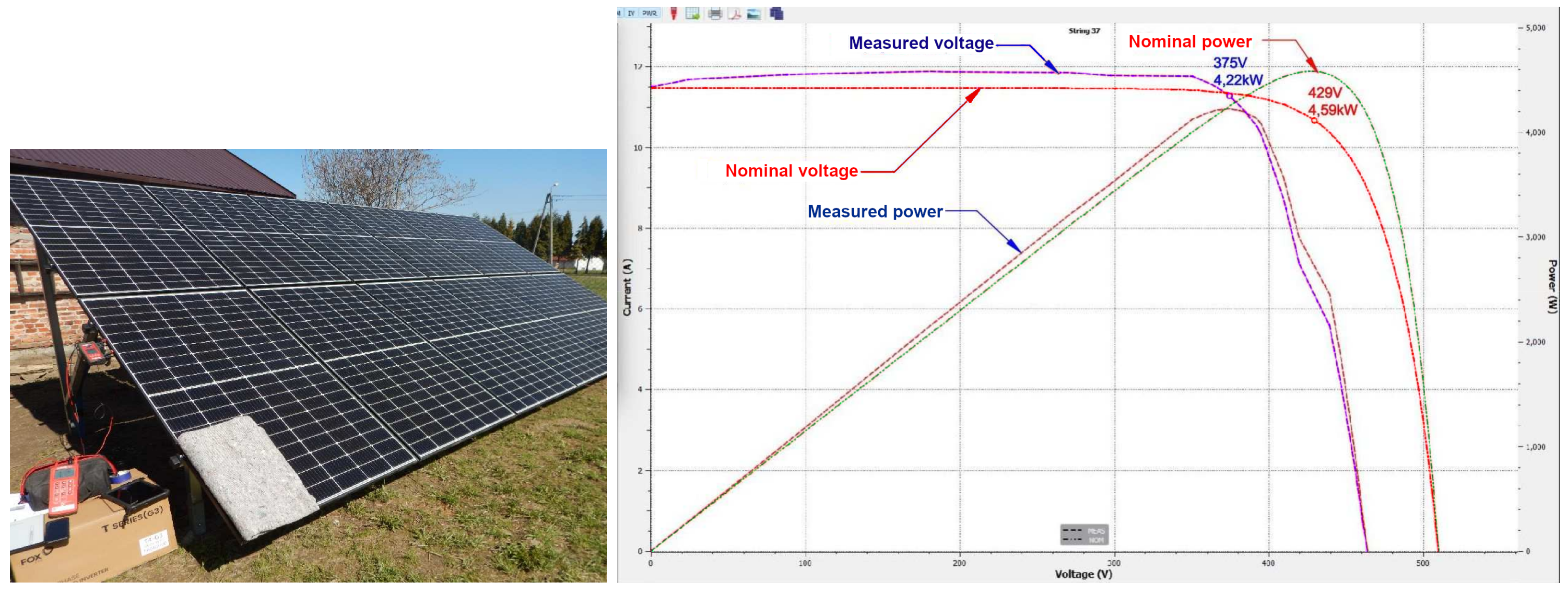
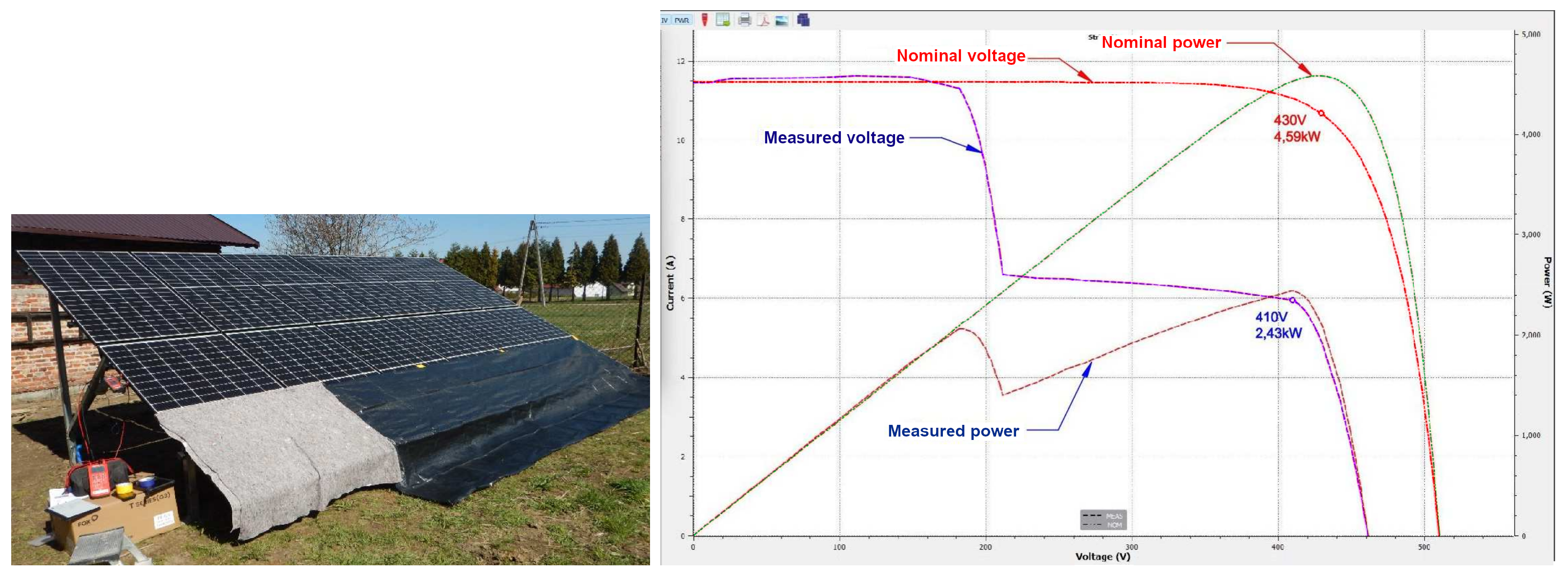
To complete the overall picture of research on losses resulting from shading, one must mention the impact of these phenomena on an installation consisting of multiple modules connected in series in a chain. Suppose the installation consists of more than one module, and the modules are done with different technologies. In that case, the effect of the shadow may have a different effect on the operation and behavior of the entire group of modules than on a single module. Consequently, the measurement result will be presented differently on the measuring equipment. We will demonstrate this using the existing ground system, constructed of 12 Chaser M6/120P (Half-Cut) photovoltaic modules of 380 W peak power each. All modules are connected in series into a single chain, oriented centrally to the south, and set at an angle of 35 degrees to the ground. Conditions during the tests were favorable, the weather stable and sunny. Radiant intensities ranged from 990–1010 W/m${}^2$. The air temperature was about 26 degrees Celsius in the sun, and the temperature of the PV modules ranged from 44–46 degrees Celsius.

We will not describe experiments analogous to those shown in Figure 5 with the shading of the installation by vegetation and small details. As a result, we found that minor shading has little effect on the efficiency of the installation, reducing its output by significantly less than 10%. Here we present only the setups which caused more substantial drops in the system performance.

Figure 7 shows the effect of covering a small section of the module on string performance. Moreover, in this case, only a small (about 9%) degradation of the performance is observed, favoring modules with Half-Cut technology.

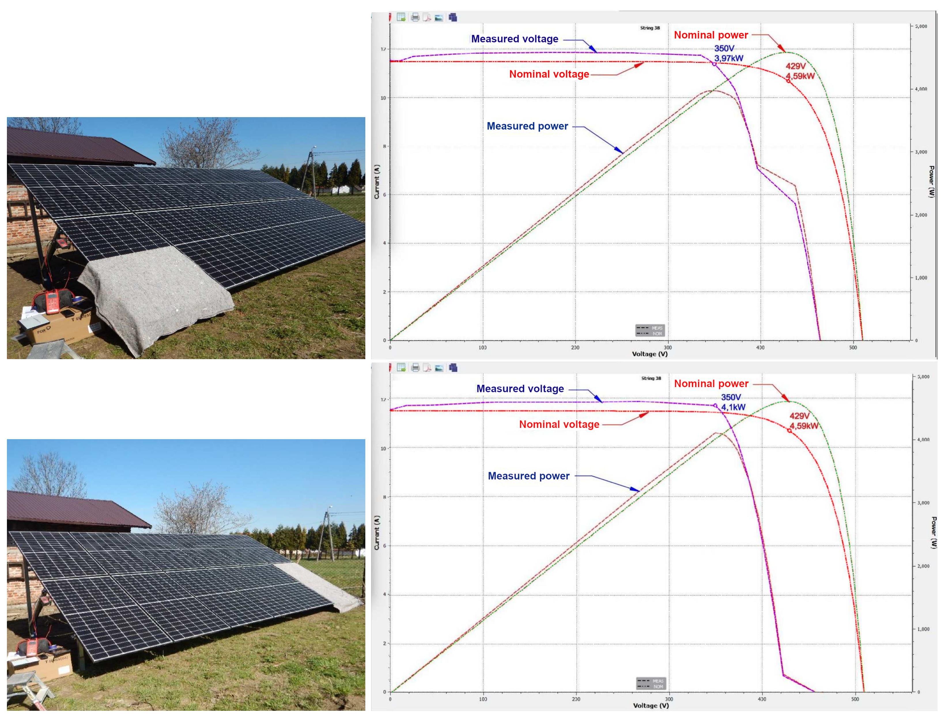
As expected, covering half of the module has a stronger impact on the installation performance. This case is documented in Figure 8 (top row). We can see that the peak power drops from 4.59 kW to 3.97 kW. More interesting is that blacking out the entire module produces similar (or even slightly weaker) effects—see the bottom row of Figure 8.

The most significant impact on the performance of the installation can be observed in the case of shading or covering the entire lower part of the string. Such a situation is presented in Figure 9. The installation still produces 2.4 kW, about half of its maximum output. In the case of standard 60-cell modules, such a situation could shut down the maximum power point tracking module of the inverter [37] due to a too-low chain voltage. Half-Cut modules, however, handle this type of problem quite efficiently.

3. Defects on Thermal Images

Thermography or infrared (IR or IRT) imaging is a non-destructive measurement technique that provides rapid, real-time imaging of PV module operation. It can be a non-contact method for diagnosing defects and problems in PV modules. For precise detection of defects, thermography can be performed under artificial illumination of the PV module and temperature distribution under different load conditions, such as short-circuited and open. However, this is an impractical approach for large installations or even small but usually difficult to access backyard systems. Luckily, thermography can also be performed during regular operation of the PV facility as an airborne scan of large systems built from many PV modules.

As already mentioned, this paper is focused on a low-cost and fast diagnostic method that will also, but not only, be practical for large, extensive, and not necessarily easily accessible installations. For this reason, we are interested in a method that will allow us to test the operation of modules under virtually any reasonable conditions. This necessitates advanced thermal image processing to minimize the impact of atmospheric conditions and uneven sunlight on the diagnostic result.

The international standard IEC TS 62446-3 [38] specifies the minimum requirements for thermal imaging cameras that can be used to inspect PV installations and also indirectly defines the correct way to take measurements by specifying the minimum resolution of the images (one pixel must image no more than 3 cm of the module edge). According to the standard, the thermographic inspection has to be executed under stable radiation of at least 600 W/m${}^2$ and weather conditions: a cloud coverage should not exceed 2/8 Cumulus and maximal 4 Beaufort wind. After short-term radiation or load changes (>10% per minute), a settling time of at least 10 min should be kept before proceeding with the inspection. However, even taking radiometric images following the recommendations of this standard does not guarantee that they will look the same for diverse farms and under different conditions for performing the fly-over.

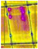
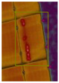
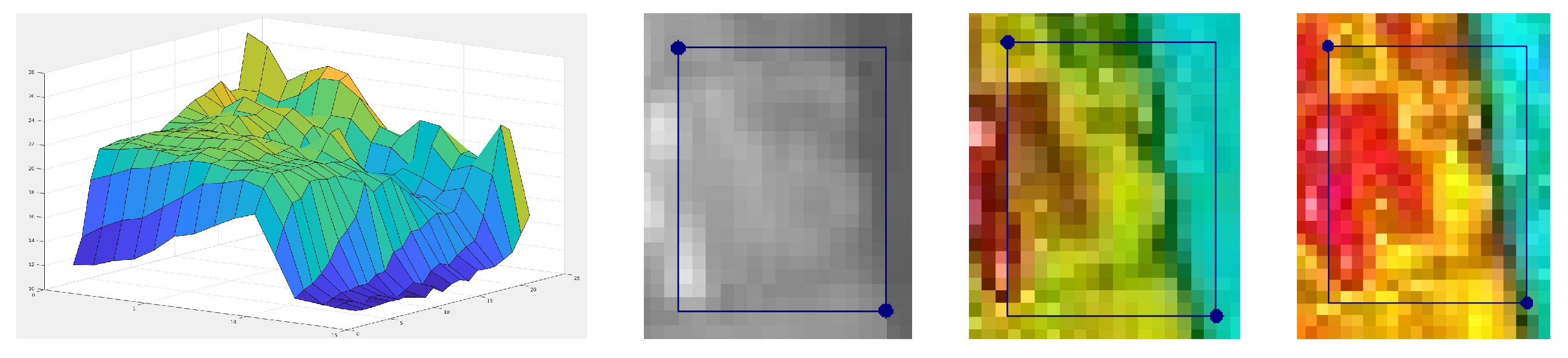
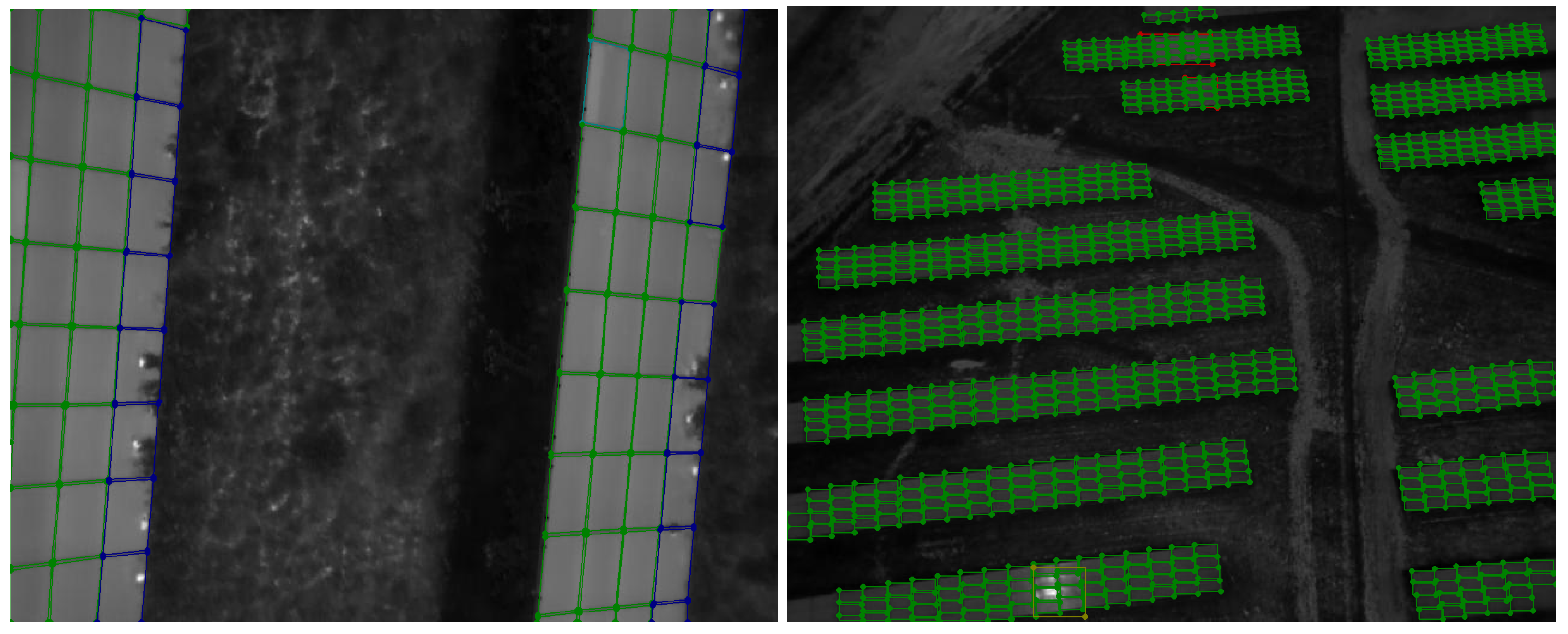
According to IEC TS 62446-3, aerial infrared thermography can reveal nine kinds of problems: overheated conductor strips, overheated cells, broken front glass of the module, overheated junction boxes, short circuits in string and substrings, disconnected string and substrings, and partial shading of modules. These problems are represented in IRT imagery by characteristic patterns; some are shown in

Table 2. Examples of IRT images of typical problems in PV installations.

Description	Temperature ${}^{+}$ [C]	Visualizations *
		Grayscale	RainbowHC	+ CLAHE ${}^{†}$
Disconnected substring
Hotspot (overheated cell)
Short circuit
Another short circuit
Partial shadow (vegetation)

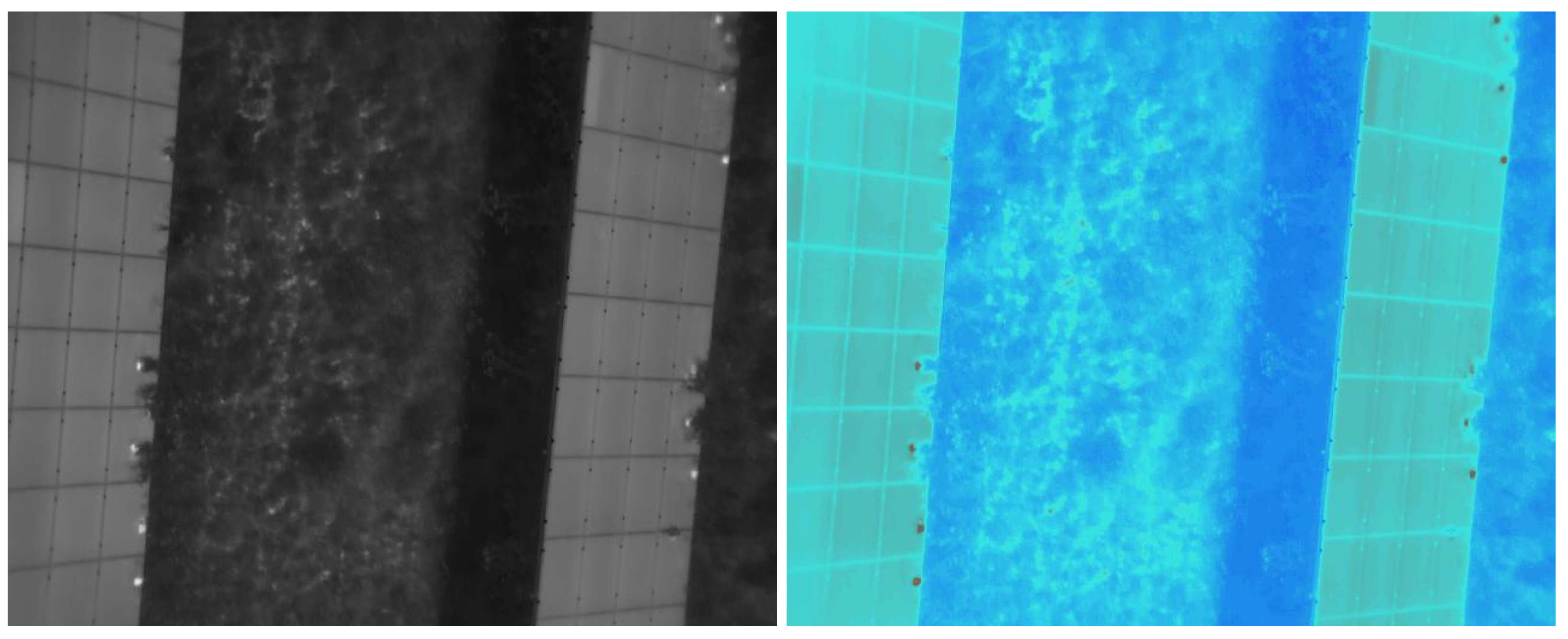
⁺ These columns show distribution of temperature on the surface of the selected PV module; ^* show visualizations of the temperature with different color palettes; ^† in this column, the Rainbow High Contrast (RainbowHC, RHC) palette [39] together with contrast limited adaptive histogram equalization (CLAHE) [40] was used.

. In the authors’ opinion, the most important function of this table is to draw the reader’s attention to the fact that the image presented on the camera’s display and stored on the memory card is just one of many possible representations of the registered temperatures. Depending on the temperature scale, color palette, and filters used, the same temperature can be depicted differently, and characteristic patterns of defects can be highlighted or blurred. To emphasize this remark in Figure 10, the DJI camera image used to create the third and fourth rows in Table 2 is compared to the temperature distribution extracted from the picture metadata.

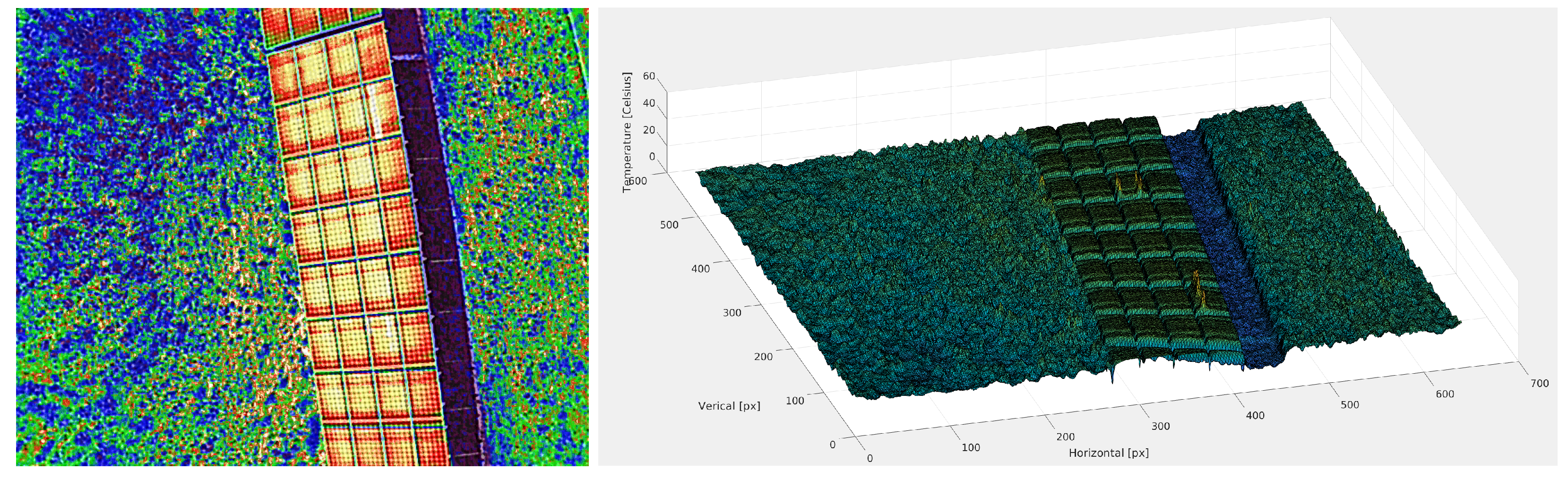
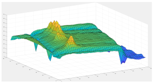
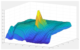
It is much easier for a human expert to evaluate images such as the one shown in the right inset of Figure 10. Together with image rotation and scaling tools, this allows precise evaluation of the area of each panel or string as a whole. Even small hotspots are visible as peaks, and the temperature scale makes it easy to assess temperature differences. However, it would be too expensive to manually evaluate several hundred or thousand of such images.

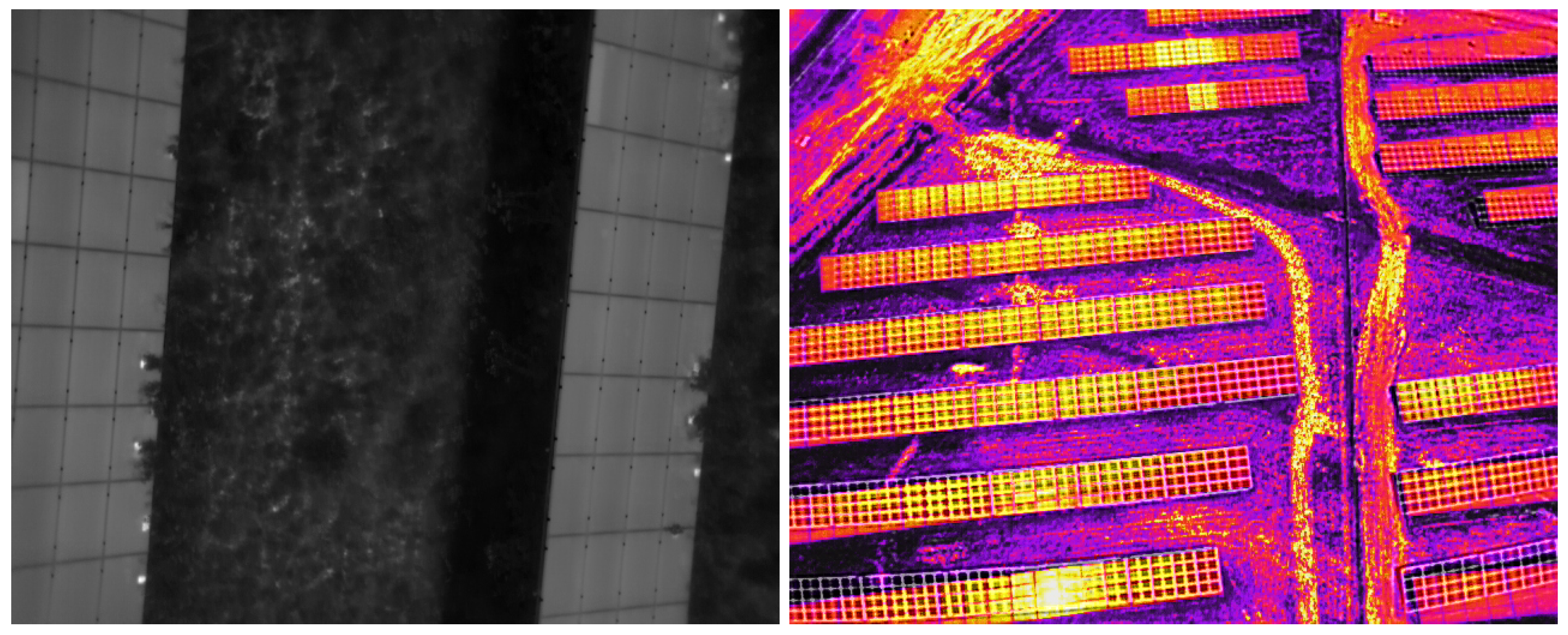
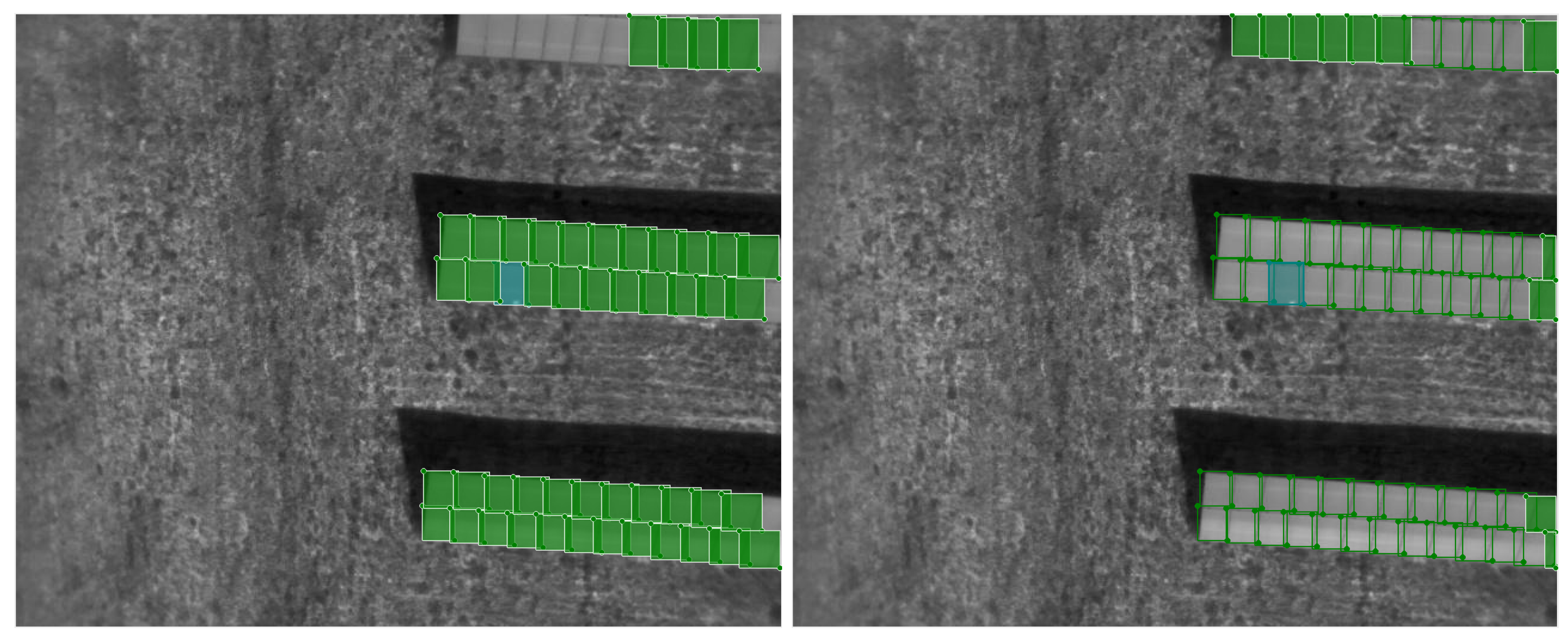
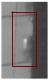
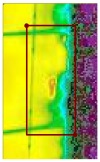
The signatures of defects of the same kind are not always clear. Comparing the third and fourth rows of Table 2, we can spot the difference, yet the origin of defects is identical and so should be their classification. The problem becomes more evident when comparing the last row of the table with a similar but bad-quality image of partial shadow shown in Figure 11. It can be said that such images do not comply with the standard because the image resolution is too low, and the 5 × 5 pixel limit for a single cell is not met. However, if we target a web-based system supporting farm inspections, dealing with poorly prepared data would also be a great advantage. Thus we do not exclude low-quality data from the learning dataset.

4. Automated Detection and Localization of Defects

The DNN

Deep Neural Networks (DNNs) have significantly popularized and dominated machine learning among data scientists and industrial applications over the past decade [41]. DNNs have found application in natural language processing, data generation (both text and images), data classification, and pattern detection. The authors study the latter example.

DNNs are neural networks consisting of more than three layers (input layer, many hidden layers, and output layer). The use of a neural network can be divided into two phases: the training phase and the use of a trained network. The network training phase requires prior preparation of training data and test data, which (in the case of DNN for detection) are pairs of files: a graphic file and a text file consisting of data describing each bounding box on a separate line. During the training phase, the numbers returned by the trained DNN are compared with the known (expected) values. Based on these results, the current DNN score is calculated, which affects the automatic update of the weights and other parameters for the next iteration of DNN training.

After completing the training, the next step is using the trained network. In that case, the input data are only image files (without additional text files), and the result from the last (output) layer is data of detected objects (described by bounding box coordinates).

The types of DNN that are best suited for detection purposes are convolutional neural networks (CNN). Their characteristic structural elements are convolutional layers, mainly responsible for extracting features from the input images. It can be assumed that a network consisting of many (not only) convolutional layers might be a better detector of the features of more complex objects (classes).

A particular example of CNN is the structure of the YOLO neural network model. This CNN was presented initially in 2015 [22] as an example of a real-time (30 frames per second or more) object detection neural network model. YOLO is a one-stage detector, which results in faster performance (unfortunately at the cost of less accuracy) because both bounding box regression and object classification are performed without earlier pre-generated region proposals (candidate object bounding boxes).

Each input image is divided into grid cells. YOLO estimates whether it contains a specific object (class) or not for each of those cells. For example, if the input image is 640 × 512 and the input layer is 416 × 416, then the image must be resized to the network input layer. After that, the image is split into 361 (19 × 19) grid cells of 21 × 21 size, and for each cell, YOLO estimates if it contains the specific object (the central point of that object) or not.

The mechanism for dealing with a situation where more than one object may be detected in a given cell is the idea of anchor boxes, i.e., predefined shapes of boxes with which YOLO tries to predict the localization of objects (classes).

It is quite possible, that several (more than one) anchor boxes in one of the cells will detect the same object. To minimize the risks of redundant object detection, YOLO uses a non-maximum suppression mechanism (NMS) to reject those bounding boxes which have a common part with others. Still, their predictions are less accurate (with a lower prediction value).

YOLO neural network model consists of several elements such as an input (which gets data in batches, e.g., 16 images simultaneously, to increase the efficiency of calculations), backbone, and neck parts responsible for features extraction and aggregation, respectively, and a head part, of which the aim is to make a prediction (object localization and classification) based on the extracted features.

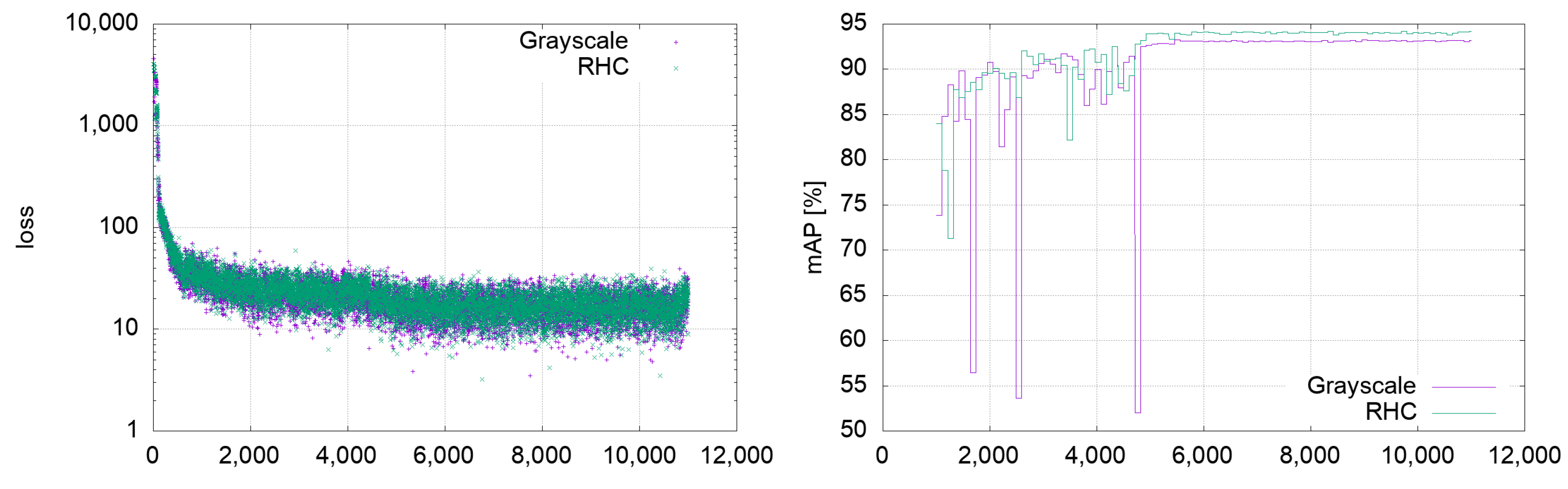
In the current research, the authors decided to use the YOLO implementation in version 4 [23], which is considered state of the art. In comparison to earlier versions, the following has been added:

• Bag of freebies (including, among others: mosaic data augmentation, self-adversarial training, drop-block);
• Bag of specials (including, among others: mish activation function [42] (which is more advanced and complicated than popular ReLU or Leaky ReLU) and Distance IoU NMS.

These additional extensions positively affect the prediction accuracy with minimal loss on the computing performance (compared to YOLOv3 [43], YOLOv4 improved mean average precision (mAP) [44] by 10%). From our point of view, the additional advantage of YOLOv4 is that it is implemented in C++, and it can be effortlessly incorporated into a larger system as a dynamically loaded library, allowing for the memory-based pipeline for image processing. Building a system based on the newer versions of YOLO (v5, v6, or v7), which are naturally implemented in Python, is much more complicated.

5. Preprocessing of Thermal Data

5.1. The Dataset

The dataset used in the experiments consists of 1060 aerial thermographic images collected at various PV farms in Poland in 2021 and 2022. The quality of the images varies; the two extreme cases are presented in Figure 12. Human experts processed all images with the help of two tools: the Thermal Studio Suite [45] with Sense Reporting plugin [46] used for image labeling, and the labelme [47] public domain graphical image annotation tool heavily extended by one of the authors. Two kinds of labeling were applied. The first one was aimed at the semantic segmentation of the images, which is not the subject of this paper. The other labeling was much simpler and oriented to be applied just for YOLO DNN. In Figure 13, both labelings are compared. It must be mentioned that the exact segmentation, shown in the left inset of Figure 13, is much more labor-intensive but also has more potential applications. It can be easily converted into the labels seen in the right inset of Figure 13, while automatically converting the bounding boxes into a segmentation is difficult. On the other side, bounding box labeling is much faster and easier. It took one 30 min to create the exact labelings shown in the left inset of Figure 13, but only less than 1 min to create what is shown in the right inset. The reader should note that segmentation is always based on the thermal, not visible image. The natural resolution of all thermograms is 640 × 512 pixels, so it is necessary to enlarge an image for manual labeling.

Seven labels were used: the “good” module, the disconnected substring, the hot spot, the short circuit of a substring, the disconnected string, the “other” fault, and the light reflex. The last label is quite special; it is not a fault of the PV module but rather the fault of the inspection, but it appears on many images and could potentially mislead the classifier. An example of the light reflex can be observed in the center of the bottom row of modules in the right inset of Figure 12 (it is also present and visible in the thermal map in Figure 13, but is almost completely covered by the labels). The original labeling is stored in XML files associated with the images. For YOLO training, these files are converted into the pure text format required by YOLO. Each label is stored in a separate line containing five numbers: the first is an integer describing the class, the next two are normalized coordinates of the box center, and the last two are normalized box width and height. Normalization involves dividing all horizontal dimensions by the width of the image, and all vertical dimensions by the height of the image.

5.2. The First Set Experiments: Two Classes

The labels were reduced to “good module” and “defective module” for the first set of experiments. Light reflexes were arbitrarily assigned to the defect group since it was assumed that it is better to “detect” a non-existent defect than to overlook an existing one. The whole dataset was divided (randomly) into two groups: 848 images for training and 212 for testing. The training dataset was enlarged by augmentation: each image was duplicated and then randomly converted. The conversion was a randomly chosen one of scaling by a random factor chosen from <0.5:0.9> or rotation by 90,180 or 270 and scaling by a random factor or by scaling by 0.25 and tiling.

YOLO has three input channels (typically RGB) and uses stacked convolutional filters. Individual filters act as feature detectors and can be (trained to be) sensitive to straight edges from dark to light or gradual transitions from green to red. Stacking them allows filters to be built for more complex features (such as PV modules). Thus, the original temperature maps from the images were converted to three-channel RGB images.

Four different conversion methods were used. In the first, the temperature of each image was independently scaled to <0:1> range with a simple formula

$$T_n=\frac{T-T_{min}}{T_{max}-T_{min}},$$

(1)

where $T_{min}$ and $T_{max}$ are the image’s minimal and maximal temperature. The normalized temperature $t_n$ was then multiplied by 255 and converted with the default grayscale color map of OpenCV [48,49] library to the three-channel grayscale image. An example of such an image is shown on the left inset of Figure 13. Additional examples are presented in the second column of Table 2.

In the second method, the Rainbow High Contrast (RHC) colormap [39] was used instead of the grayscale one. The examples of this colorization are shown in the third column of Table 2.

In the third method, the contrast limited adaptive histogram enhancement (CLAHE) [40] was applied to the image colored with RHC. CLAHE was originally defined for single-channel images. To apply it to the color one, the image is first converted to the CIELAB colorspace [50]. The CLAHE was applied to the “L” component (representing luminance), and, finally, the image was converted back to RGB.

In the fourth approach, the temperature was normalized using <0:100> range for all images:

$$T_{u}n=\frac{T-0}{100-0},$$

(2)

regardless of the values of $T_{min}$ and $T_{max}$. Then the results were converted to a three-channel image using Arctic [39] color scale. The resulted images may have black or white spots for regions where the temperature is lower than 0 (the reader should bear in mind that the Celsius scale is used) or higher than 100. Figure 14 shows the comparison of the adaptive and uniform temperature scaling.

In each experiment of the first group, the network was trained longer than required by YOLOv4 authors [23]. However, the mean average precision [23] (shown as mAP on Figure 15) was monitored to prevent loss of generality. Figure 15 shows learning curves for two example experiments: the grayscale images and the RHC images. Learning curves for other data were very similar, and the final mAP difference was lower than 1%. Figure 15 shows an unusually large final loss, which is the difference between the expected and obtained classification results. This is caused by the big diversity of the training data and the mass-scale detection of the modules shown only partially in an image. This problem is illustrated in Figure 16 where the “ground truth” image (on the left) is compared with the results of detection (on the right).

The metrics calculated for the test data in the first group of experiments are summarized in

Table 3. Metrics for the first group of experiments.

Experiment	Class	TP	FP	FN	Precision	Recall	F1
Grayscale	0	13,931	2366	1846	0.855	0.883	0.869
	1	367	115	44	0.761	0.893	0.822
RHC	0	13,482	2730	2295	0.832	0.855	0.843
	1	320	45	44	0.877	0.779	0.825
RHC + CLAHE	0	12,860	2551	2917	0.834	0.815	0.825
	1	270	38	141	0.877	0.657	0.751
Arctic	0	14,129	3006	1651	0.825	0.895	0.858
	1	277	42	134	0.868	0.674	0.759

Threshold value of IoU = 0.67; Data augmentation caused different values of TP + FN for each class. The best value of the most important recall value for the “defect” class is highlighted with the bold font.

.

Standard designations used in DNN assessments have been adopted. In assessing whether a module has been correctly located, a measure of intersection over union (IoU) is determined as the ratio of the area of the common portion of the module’s true marking, and its detection to the sum of the marked areas is primarily used. In all calculations used in this article, a threshold IoU value of 0.67 is assumed. True positive (TP) means an object is located correctly (at least 67% of its marking overlaps with the true position). False positive (FP) is the marking of an object not really in the image, and false negative (FN) is when the object in the image was not detected. Precision is calculated as the ratio of the real objects among detected ones ($p=TP/(TP+FP)$ and the recall as a ratio of existing objects being detected ($r=TP/(TP+FN)$. The most important value is the recall—the ratio of correctly located defects is shown in the seventh column of the even rows. The highest score was obtained for grayscale images. It is highlighted in Table 3.

In the second series of experiments, the network was trained to distinguish all seven classes shown in

Table 4. Labels in the database used for experiments.

Description	Number of Labels
	in Original Dataset	in Augmented Dataset
“Good” module	81,771	209,539
Disconnected substring	186	489
Hot spot	1287	3301
Disconnected string	173	413
“Other fault”	26	66
Short circuit in the substring	186	699
Light reflex	289	478

. It must be stressed that the number of samples is too low for some defects, at least for the class “other fault”. The “disconnected string” samples were also taken from just three defects. Thus the number of images is not as small, but they are similar. Thus, we cannot expect good results (i.e., high precision and high recall) for these two classes.

We have tested two sets of images: temperature converted to grayscale and temperature converted to RHC. The training process shown in Figure 17 was similar, but the RHC scale produced a slightly better mAP index. The results metrics obtained for all classes in the second set of experiments are compiled in

Table 5. Metrics for the test data for the second group of experiments.

Class	Colormap	TP	FP	FN	Precision	Recall	F1
0 (good)	grayscale	14,400	2591	1626	0.848	0.896	0.872
	RHC	14,491	2399	1543	0.858	0.904	0.881
	grayscale ${}^S$	9454	1576	33	0.857	0.997	0.922
	RHC ${}^S$	9455	1657	32	0.851	0.997	0.918
1 (faulty substring)	grayscale	31	16	2	0.660	0.939	0.775
	RHC	31	7	2	0.816	0.939	0.873
	grayscale ${}^S$	31	15	1	0.660	0.969	0.795
	RHC ${}^S$	31	6	1	0.838	0.969	0.899
2 (hotspot)	grayscale	286	37	13	0.885	0.956	0.920
	RHC	280	41	19	0.872	0.936	0.903
3 (faulty string)	grayscale	38	8	16	0.333	0.211	0.258
	RHC	38	17	25	0.405	0.447	0.425
4 (other)	grayscale	0	0	7	0	0	0
	RHC	0	0	7	0	0	0
5 (light reflex)	grayscale	38	32	4	0.543	0.905	0.679
	RHC	36	33	6	0.521	0.857	0.649
6 (short circuit)	grayscale	24	37	1	0.393	0.96	0.558
	RHC	24	6	1	0.800	0.96	0.873

^S Only images compliant with the IEC TS 62446-3 standard; threshold value of IoU = 0.67. The best value of the most important recall values for each class are highlighted with the bold font.

.

The experiments confirmed the expectation that for the correct operation of the DNN, we need to use many different examples of the objects to be detected in the training data. The lack of proper representation of class 3 and class 4 resulted in poor recognition of these defects. This problem can be solved by completing the database and teaching the network with the new one. Using the previously computed weights will speed up considerably the additional training. This method is known as transfer learning and is used by default in YOLO applications [23]. The network generally performs better processing images of good quality, but the results for images not compliant with the standard are also not disqualifying.

In the case of a normally operating PV installation, we can expect that only a small part of the installation is affected, and most panels work correctly. Thus the proper inspection of the farm should focus on the faulty modules. In the authors’ opinion, the final report should be as concise as possible. It should list all faults, specifying their position and kind (severity/origin). In addition, performing the diagnosis already during the installation’s fly-over can allow additional images to be taken, focusing on defects located earlier.

A great advantage of YOLO is the ability to analyze the images truly online. It takes less than 20 milliseconds to process a single image in detection mode using a powerful (with large memory) graphics card. The experiments described in this paper were conducted using an NVIDIA GeForce RTX 3090 Ti card with 24 GB RAM.

6. Conclusions

The main goal of this paper is to show the concept of the real-line, cheap, and effective system aimed at inspection of large or/and not easily accessible photovoltaic installations. We show that neglecting even the small problems in the module’s operation leads to measurable loss of the potential income from the plant and that an effective system can be designed with YOLO DNN. We have chosen not the newest but still competitive YOLOv4, owing to the easy incorporation of this version into a larger system.

Using a YOLO network for detecting problems in a photovoltaic installation based on thermographic images taken with a UAV should enable the development of a cost-effective solution for the ongoing inspection of even large photovoltaic farms where individual modules are not easily accessible.

YOLO allows for performing the processing of the collected material in a real online mode. Assuming that the UAV takes thermographic images no more often than once per second, YOLO makes it possible to detect defects visible in such an image even before flying the UAV to the next position. This makes possible correction of the possibly not correct detection in case of a false positive encounter. Therefore, the crucial problem of proper DNN training is to reduce the number of false negative cases. Legitimate hypersensitivity, which will result in a not-so-high precision rate, can be offset by additional diagnostics by other methods.

Two possible applications of YOLO can be imagined. In the first scenario, the YOLO is used ex-post the fly-over (or in parallel to it) and works as a filter, selecting the “suspicious” images which are later processed more precisely and comprehensively. In this scenario, using YOLO reduces the number of images that more time-consuming methods must process.

In the second scenario, YOLO is used as a standalone detector, and its speed allows to control UAV adaptively, forcing it, if a suspicious image is detected, to deviate from the pre-programmed route and take additional shots of the suspicious part of the installation from a different height, angle, or direction.

In both cases, the crucial issue of the successful application of any DNN for automated detection is the collection of an extensive, diverse database of defects. The database used in this paper was made based on material collected from almost 20 different installations for a year. Hundreds of hours were necessary to label the PV modules by human experts. However, the experiments documented in this paper showed that the database must be substantially enlarged to recognize all kinds of defects properly.

The following novelties presented in the article can be pointed out: firstly, the concept of a defect detection system operating in real-time (during the farm’s overflight, with adaptive flight path control); secondly, the emphasis on the importance of the database, and that the size, diversity, and representativeness are more important than the choice of DNN used for defect detection (all the latest architectures have essentially similar high accuracy).