Abstract
To address time delay and noise problems in control systems, in this study, we integrated an extended state filter for signal filtering into an active disturbance rejection control (ADRC) system and derived an improved ADRC approach. In addition to the active anti-disturbance and active tracking estimation functions of the existing ADRC, the proposed approach also includes active filtering and active advance prediction functions, which can filter out the effect of measurement noise on system state observation while reducing the delay between the system control output and the detection of the sensor input. We verified through an evaluation in a simulation environment that the proposed approach may be expected to achieve improved control accuracy and increase the stability of closed-loop control systems.
1. Introduction
In recent years, the theory of active disturbance rejection control (ADRC) technology has been actively developed [1,2]. Several studies [3,4] have analyzed the frequency approximation of ADRC control systems, and found that their stability margins are large and their stability is less influenced by system parameters.
It is well known that phase delay is a key issue that affects the stability of control systems. For example, the design of controllers for time-delay systems is very challenging as the time delay induces an additional phase delay [5]. Similarly, if a time delay is present between the input of the system sensing a signal and the output action of the controller, a phase delay is also introduced, which leads to an increase in the control time uncertainty and a decrease in the stability margin of the system, and may even cause the system to become unstable. Predictive ADRC was proposed to reduce the time delay between the system input and the controller output [6]. Additionally, random measurement noise is prevalent in the sensing and detection systems of realistic controllers [7,8,9], which reduces the observer bandwidth of ADRC. Furthermore, high-gain bandwidth introduces high-frequency noise, which vastly degrades the control performance of a closed-loop system, and may even destabilize the system.
The Kalman filter (KF), based on the least variance estimation, is an unbiased least variance estimation only for linear systems with Gaussian white noise. Extended Kalman filtering (EKF) is the application of the KF algorithm to linearized nonlinear systems. However, it has some limitations in dealing with nonlinear uncertain systems, because EKF is linearly expanded at the current estimate value of the state, which makes the linearization error a higher-order term of the current estimate error. When the system linearization error is large, the linearization error may become the main term in the system, which makes the filter value diverge. Therefore, when the initial estimation error and noise term are large, the stability of EKF is difficult to be guaranteed.
An ESF considers the uncertainty, process noise, and measurement noise of the system. Based on the idea of ESO, the total uncertain disturbance of the system is compensated, and the nonlinear uncertain system is changed into a linear system. Considering the process noise and measurement noise of the system at the same time, the ESF extended observation filter is derived based on the optimal prediction and estimation correction idea of the Kalman filter. ESO and KF are very mature algorithms. Using ESO disturbance compensation, the uncertain nonlinear system can be compensated to a linear system. Combined with KF filtering algorithm, it avoids the divergence and instability of the system caused by the linearization error of EKF approximation.
To address the time delay and noise problems in control systems, in this study, we derived a new anti-disturbance algorithm named EPADRC, the core idea of which is to incorporate an extended state filter [10,11] used for signal filtering into the PADRC control technology. This not only reduces the delay between the system output and the controller output, but also enables adaptive adjustment of ADRC parameters, which reduces the effect of random noise on the control system, because it performs the functions of active filtering, active tracking estimation, active anti-disturbance, and active prediction.
Active disturbance rejection control algorithms have been widely used in engineering and academia, but the traditional active disturbance rejection algorithm is basically used in engineering at present. In view of the uncertainty, high-frequency process noise, and measurement noise in practical control systems, this paper proposes for the first time an intelligent combination of an ESF and PADRC to solve the problems of limited gain of ESO that lead to low tracking and control accuracy of traditional ADRC and PADRC.
An extended state filter (ESF) serves as the core of predictive ADRC technology (PADRC) with ESF, which is primarily used to filter the detection signal. However, in the new ADRC technique EPADRC proposed in this work, the ESF can not only track the system output signal and the differential state of each order, but also dynamically reject random noise generated by sensors. Thus, the EPADRC can replace existing PADRC, and the control performance can be guaranteed in the presence of the significant external disturbances, which meet the specific requirements of power-electronics-based systems.
2. Extended State Filter
ESFs are a new type of observer with filters proposed for certain multi-input and multi-output (MIMO) nonlinear systems [12,13] with continuous uncertain dynamics and discrete measurements containing noise. An ESF is both a filter and an observer. Although the system contains nonlinear time-varying uncertainty, the covariance of the ESF filter error converges, and the range of the filter error can be evaluated in real time by the parameters (gain coefficients) of the ESF filter. Moreover, if the uncertainty is an invariant constant value, an ESF can be proven to be a linear minimum variance filter.
Developed from the extended state observer (ESO) [14,15,16], an ESF improves the ESO structure by considering the nature of measurement noise, uncertain dynamics, and discrete errors present in the system, and automatically optimizes the parameters of ESO to form the ESF. The authors of [17] derived the ESF through state estimation, tracking a MIMO system from a rigorous mathematical perspective. The derivation is relatively complex and technical. Hence, in this section, we consider single-input and single-output (SISO) systems [18,19] as an example to derive a corresponding recursive ESF algorithm.
First, we consider an nth-order nonlinear time-varying uncertainty system.
where denotes the continuous state variable, y represents the discrete sampled measurement output, is the sampling time, and is the measurement noise. This is a typical hybrid system in which the observation equation is continuous and the measurement equation is discrete. In this study, we focus primarily on the filtering characteristics of the ESF under open-loop conditions, i.e., when . In this case, Equation (1) may be rewritten as
where , , .
From Equation (2) above, it may be deduced that the ESF filter was designed to estimate the system state and unknown disturbances from discrete measurement outputs in the presence of uncertainty and measurement noise . The uncertainty exists because computing the value of from the function is impossible in practical engineering, even if the model of the function is known, because the true value of the system state is unknown.
Because filtering algorithms are usually implemented via numerical calculations carried out by computers, for example, by ZOH or FOH methods, the hybrid system (2) may be equivalently converted to the following discrete form.
where , ,
, and .
The discrete error satisfies [20].
We assume that the measurement noise is a zero-mean Gaussian sequence. Taking as an extended state, system (3) is equivalent to
where , , , and .
Let the nominal model of the nonlinear function be and the relationship of to the state variables be known in advance. Then, , the nominal model of , is given as
Then, the state filter of the discrete system (5) is
where , which denotes the tracking estimates of the state variables and of system (5) at , respectively. They are also referred to as the filtered values . Equation (7) presents the extended state filter (ESF) of the hybrid system (2).
The optimal solution of , the gain of ESF, in Equation (7) is critical for the ESF algorithm. The derivation of based on the optimal recursion method and the proof of stability of the ESF is given below.
Let the estimation error of LESO be , Then, the estimation error satisfies the following equation:
The estimation error is essentially a random variable, and since are independent of each other, we consider its mean square error of the ESF:
To find the optimal gain , the extremum of is calculated, which is .
From , , eventually, the ESF observer gain is recursively given by
where [20]
, where w0 is the initial discretization error of continuous system (1), and .
, , , here .
The stability analysis of the ESF:
If the noises and are negligible, since is Hurwitz, there is certainty that a unique positive definite matrix exists, which satisfies .
The Lyapunov function is chosen as . Then, we can get
So, .
If the noise of the system is to be considered, the Equation (8) is a stochastic system and can be rewritten as:
where, .
If a real number is given, and , there exist two positive definite symmetric matrices , and let
where and are angular moments.
Assuming that the above Equation (15) can ensure that the following formula holds,
Then by recursion, we can get:
Additionally, the mathematical expectation of satisfies the following equation:
where are the largest and smallest eigenvalues of the real symmetric matrix , respectively.
In addition, the mathematical expectation of satisfies:
From Equations (17)–(19), we can get
Since there is always a real number , , satisfying
From Equations (20) and (21), it can be deduced that:
Equation (22) shows that the state tracking error of the ESF is bounded, thus proving the stability of the ESF.
The gain of LESO is based on the same pole allocation in [21]. It is known that the convergence of ESO is , where is a small positive number.
In addition, the literature [22] provides the following convergence formula for a LESO stability proof:
, where is the bandwidth of LESO.
Additionally, for the stability of generalized ESO, the convergence conclusion is as follows in reference [23]:
, where .
In summary, the convergences of [21,22,23] mentioned above are proved, and ESF is based on the minimum variance of to obtain the gain. It can be seen that .
Equations (10)–(13) constitute the ESF parametric self-seeking algorithm, which has the following important properties and advantages.
- The mean squared error of the estimation error of the ESF is bounded regardless of whether the system is linear or nonlinear, time-variant or time-invariant, whether the dynamic model is known, and whether it contains measurement noise. Furthermore, the upper bound of the covariance matrix of the estimation error can be obtained online in real time by the parameter Pk. As is well known, in practical engineering, obtaining the exact value of the estimation error is impossible, because the state of the system is unknown. Thus, ESFs can obtain the estimation error evaluation online, which is of great significance in engineering.
- ESF can actively estimate the nonlinear part of the system (2), whereas other existing filters usually require an accurate model of the nonlinear part. Hence, ESF provides a new approach to deal with nonlinear unknown dynamics, whereas other filters have divergent filter values for large ranges of uncertain systems.
- Using ESO disturbance compensation principle, ESFs transform the uncertain nonlinear system into a linear system. Combined with a KF filtering algorithm, it avoids the divergence and instability of the system caused by the linearization error of EKF approximation.
In this way, another salient advantage of the ESF over the extended Kalman filter (EKF) is that it does not require linearization of the system model, which avoids complex computations and linearization errors. In fact, the convergence of the traditional EKF is only guaranteed for approximately linear systems. The ESF is not subject to this limitation, because it inherits the core idea of ESO—extending the nonlinear part into a new state. That is, ESF guarantees consistency (i.e., ), whereas EKF does not guarantee consistency, and its estimation error may be divergent.
- 4.
- The smaller the choice of (P0, Qk, Rk) when Equation (13) is satisfied, the smaller the PK and the better the designed ESF, as may be observed from Equation (12). Thus, P0, a diagonal array, is taken as small as possible to exceed the required variance of the initial estimation error, which is physically meaningful.
- 5.
- When the nonlinear uncertainty function is constant and the initial value of the system state variable is known, the ESF is the linear minimum variance filter. That is, when , , , the ESF is the linear minimum variance estimator of . Conversely, the ESF is the optimal tracking estimator for a system under constant total perturbations.
- 6.
- If , then , where P is the unique solution to the following Riccati equation.
It can be concluded that if and are consistently bounded, and their bounded values are and , respectively, then the consistent bound of is the solution to the Riccati Equation (23) above.
Further analysis indicates that the EKF observer gain matrix Kk also converges to a constant matrix
which is defined as the stability factor of the ESF. Additionally, θ is chosen based on the principle that P is minimized according to Equation (13).
As may be deduced from this analysis, the purpose of considering the extended state in ESF is to estimate the uncertainty term in the model in real time. Thus, its tracking estimation of the state variables is not affected by the bias resulting from the uncertainty and nonlinearity of the model, because linearization processing is not required. Hence, a filter designed in this manner does not depend on the exact model of the system, thereby avoiding the complex calculations and linearization error involved. Thus, the filter is a self-adaptive filter with self-seeking optimization, which can ensure the convergence and tracking by the filter of the state variables submerged in the measurement noise.
3. EPADRC Algorithm Incorporating ESF Filtering
A practical discrete system implementation would involve a strict time constraint such that the delay between the sensor input and the controller output should be as small as possible, which implies that the computational time consumption of the controller should be minimized. Owing to the observer-based approach, the ADRC controller has a greater computational complexity than the conventional proportional-integral-derivative (PID) controller. Thus, we aim to reduce the computational complexity of ADRC, and propose improved methods to reduce the delay between input and output in this work.
Furthermore, as random measurement noise is prevalent in the sensing and detection system of the real controller, a high-gain bandwidth introduces high-frequency noise, which significantly degrades the control performance of closed-loop systems, and can lead to system instability. Thus, such noise reduces the observer bandwidth of ADRC.
In this section, we describe our approach to fuse the ESF filter with the PADRC control technology to constitute a new anti-disturbance control technology. Because this new technology is the first new ADRC control technology proposed in this work, we refer to it hereafter as EPADRC control technology. In this section, we introduce the derivation process of EPADRC, and present that the results of simulations conducted verify that EPADRC can perform active filtering, active tracking estimation, active anti-disturbance, and active prediction, among other functions, as well as highly dynamic and high-accuracy performance.
3.1. Predictive ADRC Techniques
For nonlinear uncertain systems, compared to traditional ADRC, the PADRC has the advantage of leading the phase and reducing the input and output delay of the entire system. The literature [24] adopts the ZOH method to realize advanced observation of ESO, while PADRC is advanced predictive control of the whole control algorithm, including not only advanced prediction of the ESO part, but also advanced predictive control processing of the control law calculation part.
In applications with a fixed sampling frequency, the performance of the controller can be improved by reducing the delay between obtaining the system output signal and refreshing the controller output signal (which is also the system input signal) within a single sampling cycle. The input-output lag does not necessarily depend on the entire computation of the controller algorithm, but rather on the necessary computation required to obtain the controller output, whereby the tedious and complex computation can be performed whenever possible in the remaining time of the sampling cycle after the controller output refresh. Thus, we propose a PADRC control technique with prediction followed by correction.
We consider a second-order nonlinear time-varying uncertain system given as follows.
where , , .
This is a continuous time system, where denotes the continuous state variable , and y denotes the system output. Its corresponding PADRC loop iteration algorithm is given as follows.
where , , , , , and , , , .
Because the matrices , , , and can be computed ahead of the control algorithm, only a single multiplication and subtraction operation is performed at time , and the other complex calculations are performed after the ADRC controller output is refreshed, which significantly reduces the time delay between the system output and the controller output . In contrast, the delay between the feedback system output and the input is an important factor that affects the dynamic tracking accuracy of the system.
3.2. Theoretical Derivation of EPADRC Algorithm with an ESF
The derivation in this section includes a new EPADRC control algorithm that combines an ESF with PADRC. EPARC aims to improve the filtering performance, uncertainty compensation, phase advance, and system stability of the whole system for nonlinear and uncertain systems.
Here, we consider nth-order nonlinear time-varying uncertain systems.
where , , , .
This is the continuous time system, where denotes the continuous state variable and y represents the system output.
By the ZOH or FOH methods, the continuous system (18) can be equivalently converted to the following discrete form.
where and . Moreover,
The linearized discrete error satisfies
We assume that the measurement noise is a zero-mean Gaussian sequence. Taking as an expansion state, the system (28) is equivalent to
where , , , , .
For the discrete system (28), the terms , , and are added to the ESF covariance array for consideration. Its corresponding discrete time-extended state filter DESF is given as:
where denotes the state variables of the system (30) and the filtered values of at , respectively.
Through the derivation in Section 3.2, we know that the ESF observer gain is recursively given by
of which
In the dependencies given above, the matrix inequalities like X > Y, it means that every element of X is larger than that in Y if X and Y are matrixes.
Here, contains the estimate the extended state . Then, we can obtain its estimation error dispersion equation,
As can be deduced from the estimation error Equation (36), the characteristic roots of the matrix determine the decay process of estimation error dynamics. The observer gain determines the pole configuration of the matrix , while can be obtained automatically from Equation (32) based on the magnitude of the noise variance, indicating that the ESF has an automatic optimal configuration of the poles of the matrix.
Siemens engineers have been using the delay of the signal to lead to a deadband, the existence of which may render the control loop unstable. To reduce unnecessary time delay, we adopted the “advance prediction” and “current correction” strategy introduced above. Similar to the basic idea of Kalman filtering, the process of refreshing and outputting a filtering result is divided into two steps. First, the prediction phase is performed, in which the predicted value is obtained based on the latest measurement at time k–1. Second, the correction phase is performed, in which the predicted value is corrected based on the latest current measurement output to obtain the final estimate .
We substitute the prediction expression of Equation (37) into the correction expression to obtain
For Equation (38), we simplify the Digital Linear ESO (DLESO) as
where .
For the nth-order system of Equation (37), we generally use the linear state feedback control law given as
where , . Then, Equation (40) can be simplified as
The structure of the improved ADRC controller is presented in Figure 1.
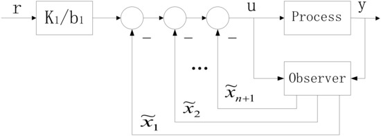
Figure 1.
Diagram of the improved ADRC structure.
Comparing Equations (40) and (41), through matrix transformation, we can convert the new estimated variable from the previously estimated variable .
where . From Equation (39), we obtain DLESO with the new estimated variable as the estimated value of the state variable
where , , .
If the matrices , , and can be precalculated ahead of the control algorithm, resource-consuming calculations such as the division of the state variables with and the multiplication with in the feedback control law (40) can thus be avoided, thereby greatly reducing the execution time of the algorithm. Because the value of the desired output at each time point is known in advance, can be computed before the algorithm execution time point, which can further improve the operational efficiency of the controller. Finally, the simplified control feedback law may be obtained as given in Equation (30).
Because the estimated state variable must be updated at each time point according to Equation (43) and the controller output is calculated using Equation (40), further optimization of the control algorithm is required.
Substituting Equation (43) directly into Equation (44) yields
As may be observed from Equation (44), the control output depends not only on the system output and the system output expectation at the moment of , but also on and at the moment of . A method that can compute with low latency is required for this purpose; at the moment of , it must precompute the part of that can be computed and correct with the current value after obtaining the system measurement output and the system output expectation at time to improve the computational efficiency of .
Normally, the system output expectation setting is known, and the calculation can be further optimized by calculating the term related to in advance at the moment of so that only the system measurement output is involved in the update of the control output at the moment of . Then, we adopt the prediction and correction to refresh the output, which is obtained from Equation (44) as:
where
The state estimate is updated using the forecast term correction, the update equation of which is given by (46).
where
Substituting Equation (48) directly into Equation (46), the prediction term for the control output is derived as
According to Equation (47), the estimated state prediction term described in Equation (49) is expressed as
Then, Equations (45), (47), (49), and (50) form the ADRC controller loop iteration algorithm, as given below.
Incorporating the recursive Equations (32)–(34) for the ESF gain derived in Section 2 into Equation (51), a new ADRC technique with self-adaptive filtering and state and control output prediction with optimal time delays is derived as follows, which we refer to as EPADRC.
3.3. Convergence of EPADRC
Since the control law of EPADRC adopts the feedforward compensation of disturbance, which is obtained by ESF observation, the nonlinear uncertain system (1) is approximately transformed into a linear series integral type:
According to Equation (40), the feedback control law of linear system (54) can be obtained as follows:
Further, the closed-loop transfer function of the system can be obtained as follows:
Then, the error transfer function is:
For step input, the flowing formula can be obtained by using the final value theorem:
So, it has been proven above that EPADRC is stable.
4. Simulation and Analysis of Results
Here, we consider a second-order nonlinear system as given below.
We considered the following simulated experimental scenario. The desired trajectory was set to a sine signal and a step signal , and the measured noise variance comprised several combinations of σ = 0.0, σ = 0.001, and σ = 0.01. The sampling time was 1 ms, and the system (59) was a closed loop controlled using PADRC and EPADRC, respectively. The results of the simulation are shown in Figure 2, Figure 3, Figure 4, Figure 5, Figure 6 and Figure 7.
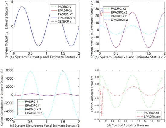
Figure 2.
Comparison of PADRC and EPADRC dynamic control performance without measurement noise.
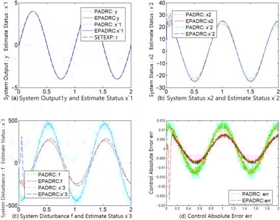
Figure 3.
Comparison of PADRC and EPADRC dynamic control performance for measurement noise σ = 0.00.
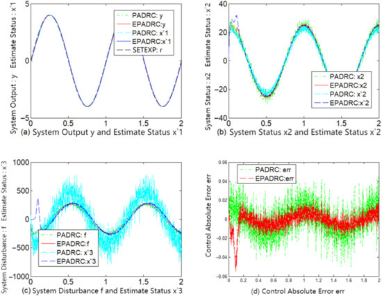
Figure 4.
Comparison of PADRC and EPADRC dynamic control performance for measurement noise σ = 0.01.
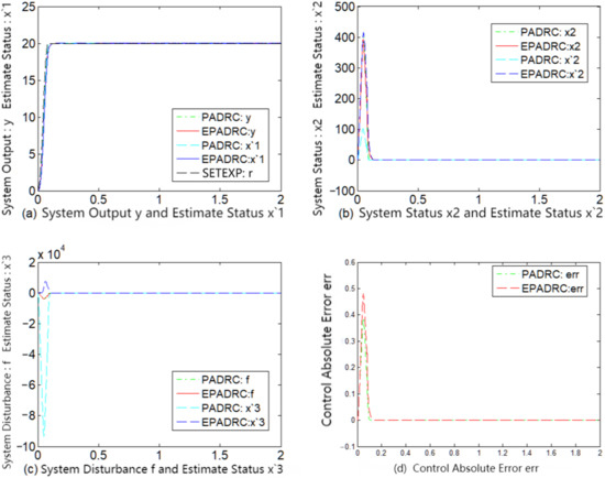
Figure 5.
Comparison of PADRC and EPADRC steady-state control performance without measurement noise.
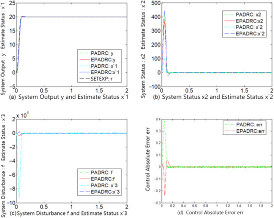
Figure 6.
Comparison of PADRC and EPADRC steady-state control performance for measurement noise σ = 0.001.
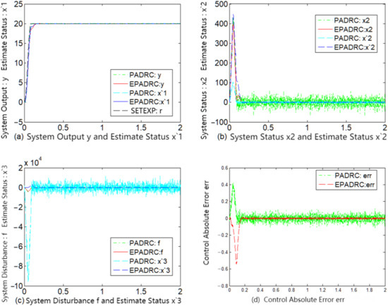
Figure 7.
Comparison of PADRC and EPADRC steady-state control performance for measurement noise σ = 0.01.
A comparative analysis of the subfigures (d) of each of Figure 2, Figure 3, Figure 4, Figure 5, Figure 6 and Figure 7 indicates that the control accuracy of EPADRC is higher than that of PADRC (except for the initial stage of the controller output, when the peaking phenomenon exists. In the actual project, to avoid the initial peaking phenomenon, the output was set to zero in the initial stage of time, both in terms of dynamic and stable control accuracy). In the initial stage, the control error of EPADRC is large, because the initial value of ESF observer gain is zero, and a short period of time is required it to seek the optimal value. Once the ESF automatically seeks the optimal value of the observer gain, its tracking accuracy greatly improves over time.
By comparing the subfigures (c) of each of Figure 2, Figure 3, Figure 4, Figure 5, Figure 6 and Figure 7, it may be deduced that EPADRC exhibited a high accuracy in estimating the unknown perturbation tracking, and thus the control error of EPADRC was smaller than that of PADRC.
As may be deduced from the subfigures (a), (b), (c), and (d) of each of Figure 2, Figure 3, Figure 4, Figure 5, Figure 6 and Figure 7, the tracking estimates of EPADRC for each state of the system were less affected by measurement noise, and the output state estimates were thus closer to the true values, thereby exhibiting better filtering capability. Conversely, the state tracking estimates of PADRC were sensitive to measurement noise, and thus the tracking estimation errors were larger compared with EPADRC.
These results demonstrate that EPADRC outperformed PADRC from the perspective of theory and simulation experiments, whereas PADRC outperformed the traditional ADRC because it has less delay between the system output measurement signal and the input control signal. Furthermore, among the three, EPADRC exhibited the best control and filtering performance.
In addition, the gain of ESF in EPADRC is the real-time optimal gain based on the minimum variance of the observation error, considering the system process noise and measurement noise. For traditional ADRC (including PADRC), the coincidence pole assignment proposed by Professor Gao Zhiqiang [25] is generally used to obtain the relationship between ESO gain and equivalent bandwidth , and then the equivalent bandwidth is manually adjusted to obtain ESO gain. The ESO gain obtained by this method is not optimal, and it is difficult to debug the optimal gain of ESF manually.
5. Conclusions
Based on a rigorous analysis and investigation of ESF, in this study, we have proposed the idea of incorporating an ESF filter in a PADRC closed-loop control system, and derived a new ADRC algorithm named the EPADRC control technique through an analysis of the optimization process of ADRC algorithm. Moreover, we have seamlessly incorporated the recursive algorithm of the ESF gain into ADRC.
We comparatively studied the tracking and filtering characteristics of EPADRC and PADRC through simulations in MATLAB, which verified that the algorithm not only possesses the functions of traditional ADRC, including active anti-disturbance and active tracking estimation, but also active filtering and active advance prediction. These new functions can filter out the effect of system measurement noise on observations of the system state, and concurrently reduce the delay between the system control quantity output and the detection of sensor inputs, thereby improving the control accuracy of the system. Hence, the proposed approach may be expected to increase the stability of closed-loop control systems.
Author Contributions
Conceptualization, S.S. and P.C.; methodology, S.S.; validation, C.Z. and L.G.; formal analysis, P.C. and Z.Z.; writing—original draft preparation, P.C.; writing—review and editing, S.S. and Z.Z.; project administration, Z.Z.; funding acquisition, P.C. and S.S. All authors have read and agreed to the published version of the manuscript.
Funding
This research was funded by the National Natural Science Foundation of China (Grant No. 51909245, 62003314); the Fundamental Research Program of Shanxi Province (Grant No. 201901D211244, 202103021224187), the Aeronautical Science Foundation of China (Grant No. 2019020U0002).
Data Availability Statement
Not applicable.
Conflicts of Interest
The authors declare no conflict of interest.
References
- Chen, S.; Xue, W.; Zhong, S.; Huang, Y. On comparison of modified ADRCs for nonlinear uncertain systems with time delay. Sci. China Inf. Sci. 2018, 61, 70223. [Google Scholar] [CrossRef]
- Wu, Z.-H.; Deng, F.; Guo, B.-Z.; Wu, C.; Xiang, Q. Backstepping Active Disturbance Rejection Control for Lower Triangular Nonlinear Systems with Mismatched Stochastic Disturbances. IEEE Trans. Syst. Man Cybern. Syst. 2021, 55, 2688–2701. [Google Scholar] [CrossRef]
- Tian, G.; Gao, Z. Frequency Response Analysis of Active Disturbance Rejection Based Control System. In Proceedings of the 16th IEEE International Conference on Control Applications Part of IEEE Multi-Conference on Systems and Control, Singapore, 1–3 October 2007; pp. 1595–1599. [Google Scholar]
- Shi, S.; Li, J.; Zhao, S. On Design Analysis of Linear Active Disturbance Rejection Control for Uncertain System. Int. J. Control Autom. 2014, 7, 225–236. [Google Scholar] [CrossRef]
- Zhao, S.; Gao, Z. Modified active disturbance rejection control for time-delay systems. ISA Trans. 2014, 53, 882–888. [Google Scholar] [CrossRef] [PubMed]
- Wu, J.-A.; Tian, C.; Yan, P. A Predictor-Based ADRC for Input Delay Systems Subject to Unknown Disturbances. In Proceedings of the 2018 Chinese Automation Congress (CAC), Xi’an, China, 30 November–2 December 2018; pp. 231–236. [Google Scholar]
- Ramírez-Neria, M.; Madonski, R.; Shao, S.; Gao, Z. Robust Tracking in Underactuated Systems Using Flatness-Based ADRC with Cascade Observers. J. Dyn. Syst. Meas. Control 2020, 142, 091002. [Google Scholar]
- Song, J.; Zhao, M.; Gao, K.; Su, J. Error Analysis of ADRC Linear Extended State Observer for the System with Measurement Noise. In Proceedings of the 21st IFAC World Congress on Automatic Control—Meeting Societal Challenges, Berlin, Germany, 11–17 July 2020; pp. 1306–1312. [Google Scholar]
- Grelewicz, P.; Nowak, P.; Czeczot, J.; Musial, J. Increment Count Method and Its PLC-Based Implementation for Autotuning of Reduced-Order ADRC with Smith Predictor. IEEE Trans. Ind. Electron. 2021, 68, 12554–12564. [Google Scholar] [CrossRef]
- Hui, J.; Yuan, J. Kalman filter, particle filter, and extended state observer for linear state estimation under perturbation (or noise) of MHTGR. Prog. Nucl. Energy 2022, 148, 104231. [Google Scholar] [CrossRef]
- Xue, W.; Zhang, X.; Sun, L.; Fang, H. Extended state filter based disturbance and uncertainty mitigation for nonlinear uncertain systems with application to fuel cell temperature control. IEEE Trans. Ind. Electron. 2020, 67, 10682–10692. [Google Scholar] [CrossRef]
- Liu, Y.; Zhu, Q. Adaptive neural network asymptotic control design for MIMO nonlinear systems based on event-triggered mechanism. Inf. Sci. 2022, 603, 91–105. [Google Scholar] [CrossRef]
- Dutta, L.; Kumar Das, D. Nonlinear disturbance observer-based adaptive nonlinear model predictive control design for a class of nonlinear MIMO system. Int. J. Syst. Sci. 2022, 53, 2010–2031. [Google Scholar] [CrossRef]
- Mandali, A.; Dong, L. Modeling and Cascade Control of a Pneumatic Positioning System. J. Dyn. Syst. Meas. Control 2022, 144, 061004. [Google Scholar] [CrossRef]
- Li, H.; Li, S.; Lu, J.; Qu, Y.; Guo, C. A Novel Strategy Based on Linear Active Disturbance Rejection Control for Harmonic Detection and Compensation in Low Voltage AC Microgrid. Energies 2019, 12, 3982. [Google Scholar] [CrossRef]
- Ran, M.; Wang, Q.; Dong, C.; Xie, L. Active disturbance rejection control for uncertain time-delay nonlinear systems. Automatica 2020, 112, 108692. [Google Scholar] [CrossRef]
- Bai, W.; Xue, W.; Huang, Y.; Fang, H. The Extended State Filter for A Class of Multi-Input Multi-Output Nonlinear Uncertain Hybrid Systems. In Proceedings of the 33rd Chinese Control Conference, Nanjing, China, 28–30 July 2014. [Google Scholar]
- Li, X.; Wen, C.; Zou, Y. Adaptive Backstepping Control for Fractional-Order Nonlinear Systems with External Disturbance and Uncertain Parameters Using Smooth Control. IEEE Trans. Syst. Man Cybern. Syst. 2021, 51, 7860–7869. [Google Scholar] [CrossRef]
- Hill, R.; Luo, Y.; Schwerdtfeger, U. Exact recursive updating of state uncertainty sets for linear SISO systems. Automatica 2018, 95, 33–43. [Google Scholar] [CrossRef]
- Bai, W.; Xue, W.; Huang, Y.; Fang, H. On extended state based Kalman filter design for a class of nonlinear time-varying uncertain systems. Sci. China Inf. Sci. 2018, 61, 042201. [Google Scholar] [CrossRef]
- Zheng, Q.; Chen, Z.; Gao, Z. A practical approach to disturbance decoupling control. Control Eng. Pract. 2009, 17, 1016–1025. [Google Scholar] [CrossRef]
- Xue, W.; Huang, Y. On Performance Analysis of ADRC for Nonlinear Uncertain Systems with Unknown Dynamics and Discontinuous Disturbances. In Proceedings of the 32nd Chinese Control Conference, Xi’an, China, 26–28 July 2013; pp. 1102–1107. [Google Scholar]
- Guo, B.-Z.; Zhao, Z.-L. On the convergence of an extended state observer for nonlinear systems with uncertainty. Syst. Control Lett. 2011, 60, 420–430. [Google Scholar] [CrossRef]
- Miklosovic, R.; Radke, A.; Gao, Z. Discrete Implementation and Generalization of the Extended State Observer. In Proceedings of the 2006 American Control Conference, Minneapolis, MN, USA, 14–16 June 2006; Volume 6, pp. 2209–2214. [Google Scholar]
- Gao, Z. Scaling and Bandwidth-Parameterization Based Controller Tuning. In Proceedings of the 2003 American Control Conference, Denver, CO, USA, 4–6 June 2003; pp. 4989–4996. [Google Scholar]
Publisher’s Note: MDPI stays neutral with regard to jurisdictional claims in published maps and institutional affiliations. |
© 2022 by the authors. Licensee MDPI, Basel, Switzerland. This article is an open access article distributed under the terms and conditions of the Creative Commons Attribution (CC BY) license (https://creativecommons.org/licenses/by/4.0/).