Article

Analysis of Energy Loss on a Tunable Check Valve through the Numerical Simulation

1
Faculty of Mechanical Engineering, Cracow University of Technology, 31-155 Cracow, Poland
2
PONAR Wadowice S.A., 34-100 Wadowice, Poland
*
Author to whom correspondence should be addressed.
These authors contributed equally to this work.
Energies 2022, 15(15), 5740; https://doi.org/10.3390/en15155740
Submission received: 13 July 2022 / Revised: 1 August 2022 / Accepted: 2 August 2022 / Published: 8 August 2022
(This article belongs to the Special Issue Computer-Aided Design of Hydraulic Systems)

Abstract

:
The article presents a study of the flow through a tunable check valve used as a hydraulic lock in a system with an actuator. Special attention is given to energy losses of the liquid stream in the poppet gap. In the first stage of the research, CFD methods were used to determine the speed and pressure distributions for the fixed values of the input flow rate and the poppet position. The values of the jet angle and pressures determined based on the CFD results were used to build a simulation model of the entire hydraulic system in Matlab/Simulink environment. The influence of the spring parameters pressing the poppet against the valve seat on the pressure drop and thus on the amount of energy lost was investigated. In particular, the spring stiffness and initial tension were studied. The obtained results were used to develop guidelines for constructing a valve prototype. Finally, the results of simulation tests were verified based on the actual valve characteristic obtained on a test bench.

1. Introduction

Check valves are widely used as flow control elements in current hydraulic and pneumatic drives. They are the key elements controlling the working medium flow direction, exposed to high pressures, and thus subjected to high forces. In hydraulic systems, especially those containing actuators subjected to long-term, continuous loads, check valves are applied as hydraulic locks, the function of which is to quickly shut off the flow and maintain complete tightness in the event of a power failure or the need to keep the current position. Such requirements apply to construction equipment, such as cranes, load-handling devices, including forklifts, conveyors, stock pickers, elevators, and manufacturing equipment, e.g., industrial presses. Studies on determining the characteristics of these valves, and thus estimating and minimizing energy losses during the flow of the working fluid through valve channels and gaps, are conducted in leading research centers. The subject of research is often related to the transient state during flow opening and the appropriate selection of parameters of simulation models. Ye et al. [1] studied transient flow characteristics of a high-pressure hydrogen check valve. In the first step, fluid flow properties during the opening process were obtained, including the velocity changes and pressure distribution. Next, fluid forces, valve spool acceleration and velocity were determined. Finally, the influence of inlet pressure on the operating characteristics of the spool was analyzed. In further work, Ye presented check valve spool-head angle optimization results in the high-pressure hydrogen storage system [2]. The transient CFD method and the moving mesh technology were used to determine flow characteristics against the spool-head angle during the opening process. In contrast, Kim and Yeong [3] provided recommendations related to the choice of an appropriate CFD mesh moving method in the check valve closing behavior modeling. Four different techniques were modeled and tested. Then the obtained results were compared, and practical conclusions were formulated.
The flow characteristics of a butterfly check valve in a small modular reactor by means of CFD method were determined by Wen et al. [4]. The authors obtained the valve loss coefficient against the valve opening angle using five different turbulence models. The research showed that the best compliance of the simulation results with experiments was obtained for the k ε model. The transient flow of check valves installed in the nuclear industry systems was also investigated by Lai et al. [5], using the unsteady CFD method. Lai analyzed a multi-receiver system in the parallel arrangement and used check valves to reduce energy consumption in the case when not all branches are put into operation. Another analysis of the characteristics of a directional poppet valve using the CFD method was presented by Gomez in [6]. The influence of the poppet cone angle on pressure and flow forces was investigated. Special attention was paid to predicting the valve behavior operating at high frequencies. It was found that with the assumed operational conditions, the cone angle has a negligible effect on pressure loss, while the flow force rises as the angle decreases. Similarly, Deng et al. [7] took up the transient opening state of a check valve under multiphase flow conditions. Deng built several candidate CFD transient models with different turbulence models, which were next subjected to probabilistic modeling to predict the check valve opening height more accurately. Moreover, Ling et al. [8] focused on the dynamics and transient states of a novel, high-speed, precise piezoelectric flow control valve.
In the field of research on the check valve design modifications, one can mention the publication by Shin et al. [9], in which the authors proposed to change the pressure valve opening control to an active driving force, which significantly improved the reliability of the studied system. In turn, Morgan et al. [10] introduced the concept of a tunable check valve for low flow, which can be used for marine nutrient sensing. The use of a permanent magnet eliminated the need for an additional power supply. Gao et al. [11] conducted a comparative analysis of two design solutions: swing and tilting check valves with systems containing compressible fluids. Based on the CFD tests performed, recommendations were formulated regarding the advantages and disadvantages of both tested solutions. Furthermore, Baluyev et al. [12] presented a study on the functional characteristics of a check valve installed in the safety system of a liquid metal cooled reactor. The research included calculations in Ansys CFX based on a scaled model and laboratory experiments. As a result, the hydrodynamic characteristics of the valve against the selected design and operational parameters were obtained. In the field of research on check valves in specific systems, Yang [13] provided a method of integrating check valves in the flapping wing membrane of a micro air vehicle. Schickofer [14] used high-order FSI simulations and low-order analytical models to examine the stability and non-linear dynamics as well as the opening and closing characteristics of a check valve in a shock absorber.
This work is a continuation of previous research conducted by the authors using the CFD method and laboratory experiments on check valves. The studies included an analysis of flow through a directional control valve consisting of four poppet seat valves [15] and a proposal of geometric modifications of an adjustable check valve [16]. This paper concerns research on a check valve designed for larger flows, with a nominal volumetric flow rate Q n o m = 360 dm3 min−1. The greatest emphasis is placed on the analysis of flow parameters, such as velocity and pressure, with special attention put on pressure losses occurring in the poppet gap.

2. Working Principle of a Tunable Check Valve

The subject of the analysis is a tunable check valve whose default design is shown in Figure 1. The flow channels are made in the body (1) closed with covers (2) and (3). The flow can occur in both directions, A-B and B-A, through the annular slot of the poppet (4). The valve opens the flow in the A-B direction against the spring (7) force and the flow forces. In contrast, unblocking the flow through the valve in the B-A direction is possible after giving an appropriate pressure control signal acting on the pilot surface (8). The signal generates a force sufficiently large for displacing the poppet. A relatively high nominal flow characterizes the analyzed valve; therefore, it was proposed to use an initial valve, including the tapered hole in the poppet, the ball (5) and the disc (6). This solution makes it possible to compensate for the pressures on both sides of the poppet before the main flow is opened.
Essential, both for the initial phase of valve opening and the total pressure losses during the flow, is the appropriate selection of the spring (7) stiffness, which generates the force of pressing the operating surface of the poppet against the edge of the seat. The second parameter affecting the flow forces, and thus the valve-opening characteristic, is the initial tension imposed on the spring.

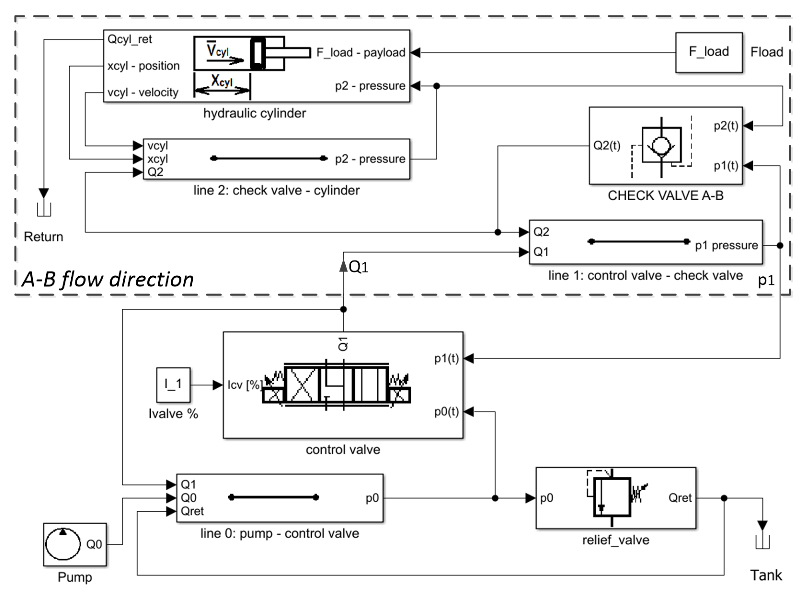
3. Mathematical Model of the System

The modeled hydraulic system includes a fixed speed pump, a control valve, the above-mentioned check valve, and a hydraulic actuator with a maximum load of 500 kN (Figure 2). The model was created according to the methodology proposed by Novak et al. [17], considering both flow directions through the check valve, A-B and B-A, respectively. The input signal is the pump flow rate. Next, equations of fluid mass conservation are written for the distinguished volumes, and equations of motion based on force balances are formulated for the valve poppet and the hydraulic cylinder piston. Flow equations through throttle slots are based on Bernoulli’s law and geometrical relations.
The input flow rate was determined, assuming the use of a piston pump with z pistons, the piston stroke rate per revolution q r e v and the angular speed ω 0 , as follows:
Q 0 ( t ) = q r e v · ω 0 ( t ) · k = 0 z / 2 1 s i n ( ω 0 · t + 2 π k z ) ,
where the angular speed ω 0 ( t ) increases linearly at the start-up time t s t a r t and then remains constant:
ω 0 ( t ) = ω n o m · t / t s t a r t for t < t s t a r t ω n o m otherwise .
The equation of mass conservation formulated for the supply line takes into account the division of the fluid stream into control valve and relief valve flow rates, Q 1 and Q r e t , respectively:
d p 0 ( t ) d t = B f / V 0 · ( Q 0 ( t ) Q 1 ( t ) Q r e t ( t ) ) .
Control valve flow rate Q 1 ( t ) is determined based on the characteristics obtained during previous studies [18], as a function of the pressure difference Δ p = p 0 p 1 and the control signal U:
Q 1 ( t ) = f ( p 0 ( t ) , p 1 ( t ) , U ) ,
while the relief valve opens in the case when the p 0 pressure exceeds the allowable range:
Q r e t ( t ) = f ( p 0 ( t ) ) .
Pressures p 1 ( t ) and p 2 ( t ) depend on the control valve setting. Depending on whether the pump is connected to port A (A-B flow direction) or port B (B-A flow direction), the mass conservation equations have the following form:
d p 1 ( t ) d t = B f / V 1 · ( Q 1 ( t ) Q 2 ( t ) ) ( A - B direction ) B f / V 1 · ( Q 1 ( t ) A c y l , r · v c y l ) ( B - A direction )
d p 2 ( t ) d t = B f / V 2 · ( Q 2 ( t ) A c y l · v c y l ) ( A - B direction ) B f / V 2 · ( A c y l · v c y l Q 2 ( t ) ) ( B - A direction ) .
Similarly, the equation of the hydraulic cylinder piston motion in both directions can be written as follows:
m c y l d 2 x c y l ( t ) d t 2 = p 2 ( t ) · A c y l p r e t ( t ) · A c y l , r φ · d x c y l ( t ) d t F l o a d ( A - B direction ) p 1 ( t ) · A c y l , r p 2 ( t ) · A c y l φ · d x c y l ( t ) d t F l o a d ( B - A direction ) .
The flow rate through the check valve depends on the poppet position and, therefore, the width of the annular gap. The force balances in the A-B and B-A flow directions are shown in Figure 3a,b, respectively.
For the A-B direction, the poppet motion equation was written as follows:
m p d 2 x p ( A B ) ( t ) d t 2 = F h s A 1 F h s A 2 F s p r F f F h d .
where hydrostatic forces acting on both sides of the poppet F h s A 1 ( t ) = p 1 ( t ) · A p A , F h s A 2 ( t ) = p 2 ( t ) · A p B . Spring force includes the initial spring tension and deflection due to poppet displacement: F s p r ( t ) = ( x s 0 + x p ( t ) ) · k s p r . The friction force, which is proportional to poppet velocity, depends on the geometry and fluid dynamic viscosity: F f ( t ) = η · Φ g · d x p d t , where the geometrical factor Φ g = π · d p · l p · ( c r p 1 ( e p / c r p ) ) 1 . Hydrodynamic force acting on the spool: F h d = ρ · Q 2 ( t ) · v a v g · c o s ( λ ) , where the average fluid velocity v a v g = 2 / ρ · ( p 1 ( t ) p 2 ( t ) ) . The methodology for determining the λ angle based on CFD results was presented in [19,20,21]. In the B-A flow direction, the equation of the poppet motion has the form:
m p d 2 x p ( B A ) ( t ) d t 2 = F h s C + F h s A 1 F h s A 2 F s p r F f + F h d .
Compared to the A-B direction, there are no differences in the hydrostatic force F h s A 2 , spring force F s p r and friction force F f formulas. The hydrodynamic force equation is also the same, except for the difference in determining the average velocity: v a v g = 2 / ρ · ( p 2 ( t ) p r e t ) . The hydrostatic force moving the valve pilot comes from the pressure transmitted through the X port: F h s C ( t ) = p 2 ( t ) · A p C , while the force acting on the left side of the poppet comes from the return line pressure: F h s A 1 ( t ) = p r e t ( t ) · A p A .

4. Check Valve Discrete Model and CFD Analysis

The CFD analyses were carried out utilizing a university research package of ANSYS/Fluent software, while the check valve geometric model was built using PTC Creo. Next, boundary conditions and the turbulence model in ANSYS/Fluent were assigned. Based on the geometric model, the initial meshing process was conducted and preliminary CFD calculations were made in order to assess the mesh quality. After the mesh parameters were finally selected, complete valve flow tests were performed for the set flow rate values.

4.1. Boundary Conditions and Turbulence Model

The following boundary conditions were set: the inlet average fluid velocity based on the input flow rate and the outlet pressure. The input velocity was assigned as perpendicular to the boundary with the Boundary Conditions/Velocity Specification Method option. The Outlet Condition/Gauge Pressure option was used to define the outlet pressure p o u t . Values of the physical model parameters are shown in Table 1.
The value of the Reynolds number determined for the given flow channel geometry, fluid viscosity ν and the flow rate range Q m i n Q m a x varies from R e m i n = 2.8 × 10 3 to R e m a x = 2.5 × 10 4 . The value of R e indicates the transient or turbulent flow; thus, the turbulence model needs to be assigned. Based on the literature related to CFD studies on hydraulic and pneumatic elements, such as a pump [22], a turbine [23], and valves [4,24,25], the standard k ε model was chosen. ANSYS/Fluent provides several variants of the k ε model. However, earlier studies of the authors on a similar, smaller-size check valve [16] have shown that the standard k ε model gives almost identical results to the RNG and realizable variants. On the other hand, the computation time, which is a crucial parameter in long-term calculations, is shorter by about 10%.
The transport equations used for determining the main factors, such as kinetic energy of the turbulence k, kinetic energy dissipation ε and turbulent viscosity μ t , can be found in many publications, e.g., [16,24,26]. Table 2 shows the parameters defining the specificity of turbulence, including intensity I (Equation (11)), length scale (Equation (12)) and other constants with values recommended by ANSYS [27].
I = 0.16 · R e 0.125 ,
= 0.07 · D H ,
where D H is the relevant hydraulic diameter, R e is the Reynolds number, and ρ is the fluid density.

4.2. Meshing and Assessing Mesh Quality

The mesh was created using irregular elements. The boundary layers were made of prisms, while the bulk flow was modeled with tetrahedrons. The pressure–velocity coupling was achieved using the pressure-based solver. The condition for convergence was to obtain values less than 10 4 for both mass and momentum residuals.
The mesh quality was assessed by comparing the results of the CFD simulation with the results of actual laboratory tests of the valve, carried out for the A-B direction at the fixed flow rate Q = 300 dm3 min−1. The pressure drop measured at the test bench was Δ p l a b = 0.66 MPa. The steady-state CFD simulations performed using the k ε turbulence model allowed us to obtain the value of pressure losses, following ISO 4411 [28].
In the beginning, the sizes of mesh elements were adopted under the general recommendations of ANSYS, obtaining values significantly different from the laboratory results. After that, using the progressive mesh refinement technique, the mesh density was gradually increased, especially in the critical areas near the valve poppet head and the seat. These activities significantly brought the CFD simulation outcomes closer to the results of laboratory experiments. However, the computation time of a single test was simultaneously extended from 30 minutes to almost 28 hours. Three representative meshes are shown in Figure 4, while the comparison of results is summarized in (Table 3).
The results obtained for cases II and III were almost identical and highly consistent with the results of laboratory tests. Since the computation time of the case II mesh was approximately 7 times shorter, this mesh was adopted for further tests. The following mesh quality parameter values were read with the Statistics/Mesh Metrics option: maximum aspect ratio 8.9 , maximum skewness 0.92 with the average value below 0.30 , the average orthogonal quality 0.92 with the minimum value of 0.68 .

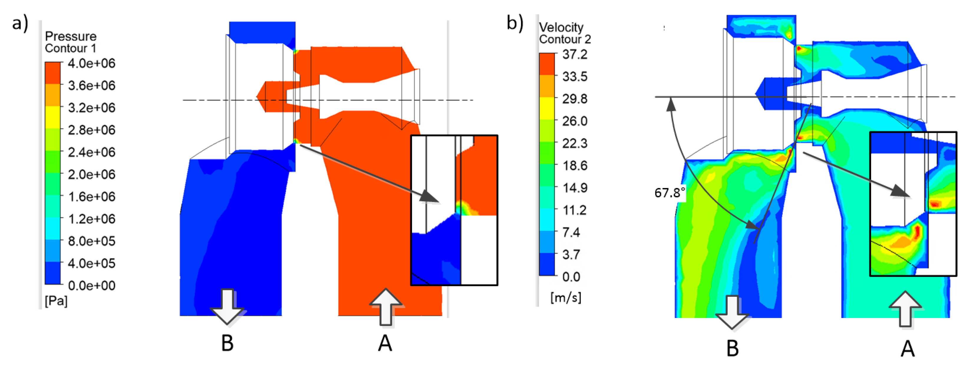
4.3. CFD Simulation Results

The CFD test plan included simulation with the nominal flow rate Q = 300 dm3 min−1 in the A-B direction and different poppet positions that define the flow gap widths: x p = 1.0 , 2.0 , 3.0 , 4.0 , 5.0 mm, respectively. In each case, the pressure and velocity distributions were obtained. The example results for x p = 1.0 , 3.0 and 5.0 mm are shown in Figure 5, Figure 6 and Figure 7, while jet angle values are summarized in Table 4.
Based on the obtained results, a linear function of jet angle against the poppet position λ = f ( x p ) was determined using linear interpolation (Equation (13)), achieving the correlation coefficient R = 0.997 and the residual sum of squares R S S = 1.4 × 10 4 . The function is valid for x p given in mm, and the resulting λ value is in radians.
λ ( x p ) = 0.0502 · x p + 1.235 .
In contrast, there is no need to determine the λ ( x p ) function for the B-A direction, as the valve is designed to fully open when a pressure signal is applied to the X port. The obtained λ ( x p ) dependency was next used to build a complete simulation model in Matlab/Simulink.

5. Simulations in Matlab/Simulink Environment

A general view of the Simulink model for the A-B flow direction, including blocks representing the main hydraulic components and reduced volumes, is shown in Figure 8. The difference in the block arrangement for the B-A direction is displayed in Figure 9.
The model includes the following components: pump, relief valve, control valve, tunable check valve and hydraulic cylinder. The reduced volumes represent lines between the elements: pump and control valve (index 0), control valve and check valve (index 1), as well as a check valve and hydraulic cylinder (index 2), respectively. The system operates at a maximum load force exerted on the actuator F l o a d = 500 kN. Figure 10 shows the input signal values in the form of a piston pump flow rate. The mean values were Q 0 = 100 , 200 , 300 , 600 , 900 dm3 min−1, marked as (1), (2) … (5), respectively. In the graph, one can observe the pulsation of approximately 6%.

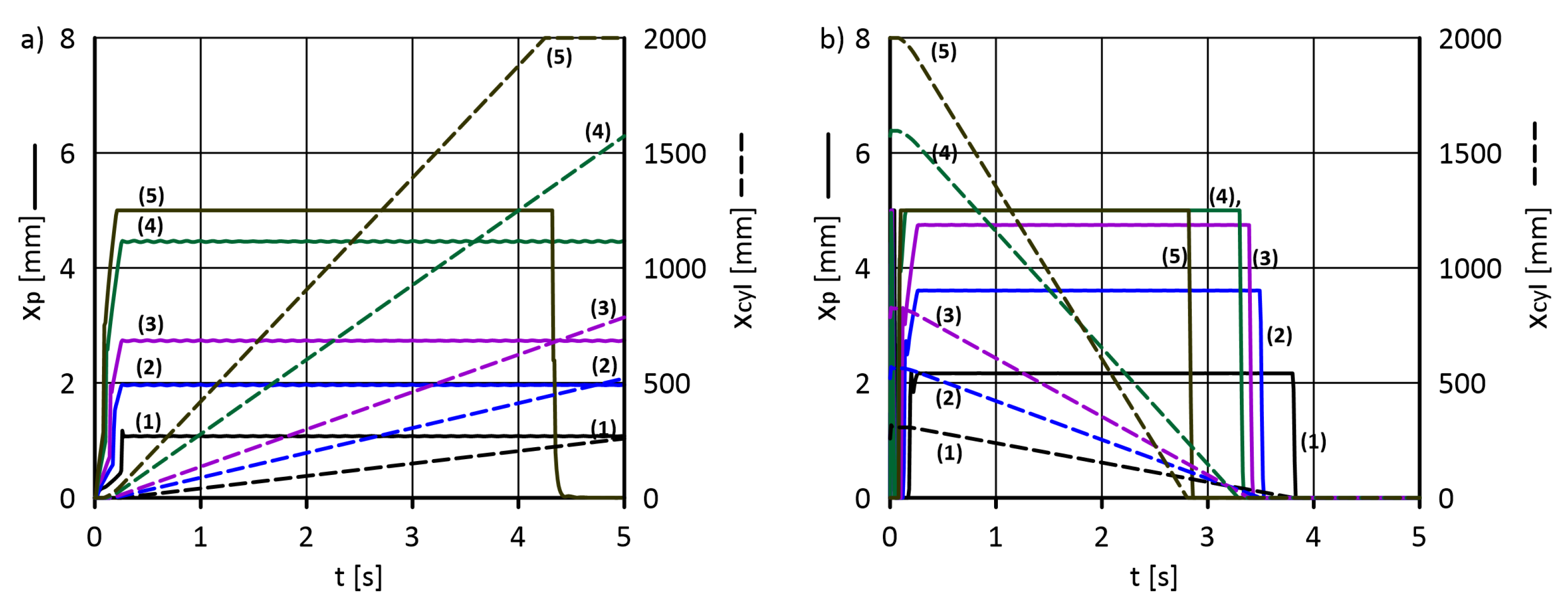
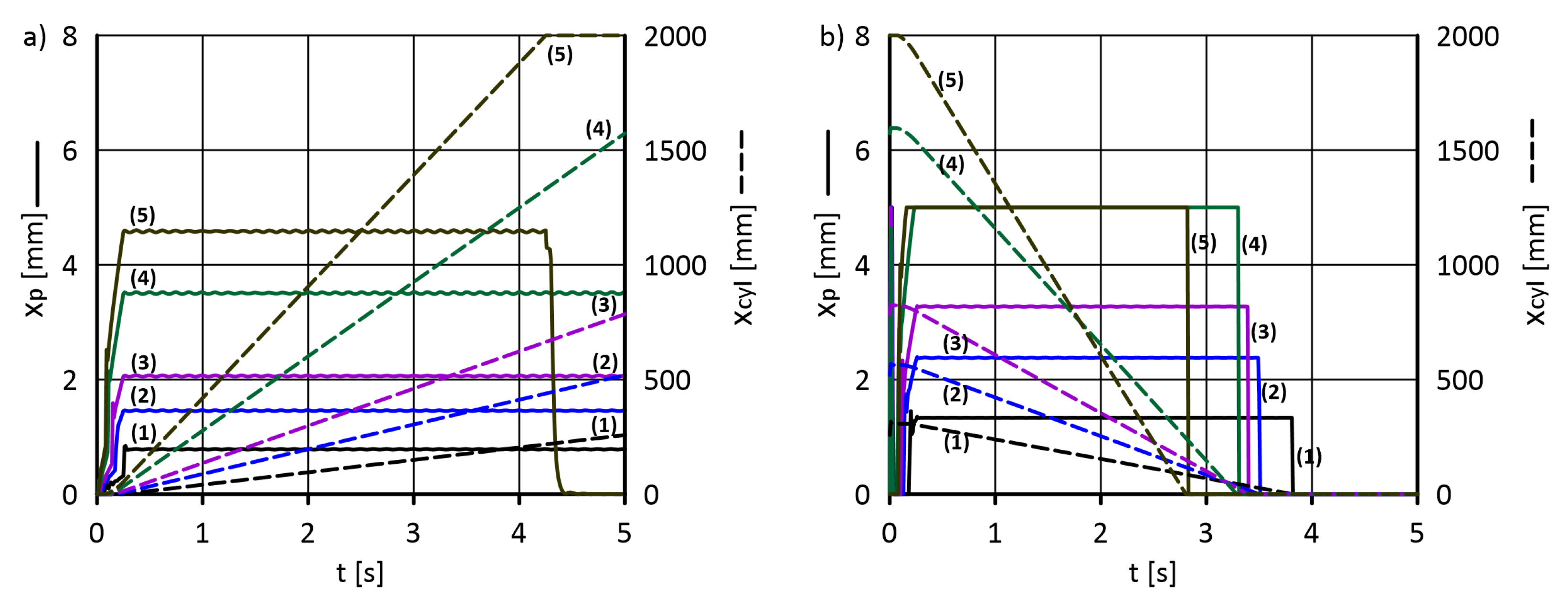
5.1. Determining the Valve Gap Width and Actuator Piston Displacement

After assigning nominal spring parameters, including stiffness of 41 N mm−1 and initial tension of 7 mm, the hydraulic system was simulated with the actuator movement in both A-B and B-A directions. The obtained courses of the check valve opening width and the actuator displacement against time for both flow directions are shown in Figure 11.
The displacement of the actuator piston in the B-A direction takes place at a higher speed due to the fluid supply to the cylinder from the piston rod side. For the same reason, the valve opening width x p is larger for the B-A flow direction. It obtains the maximum value of x p = 5.0 mm for Q 0 = 600 dm3 min−1, and for Q 0 = 300 dm3 min−1 is equals to x p = 3.8 mm. In contrast, in the A-B direction x p = 3.95 mm for Q 0 = 600 dm3 min−1 and reaches full opening for Q 0 = 900 dm3 min−1.
In two subsequent tests, the valve springs with the modified stiffness were applied. Figure 12 shows the results obtained with a softer spring (stiffness reduced by 40%, k s p r = k 1 = 24.6 N mm−1). The analogous results achieved with a 40% stiffer spring ( k s p r = k 2 = 57.4 N mm−1) are presented in Figure 13.
The results show that the spring parameters are important for the width of the flow gap. For example, at a flow rate of 300 dm3 min−1 in the A-B direction, the gap width x p varies from 2.0 mm (stiffness k 2 ) to 2.85 mm (stiffness k 1 ). In the B-A direction the difference in the opening width is even greater, from 3.1 mm to 4.8 mm. As a result, the pressure drop across the valve changes, which leads to different energy losses.

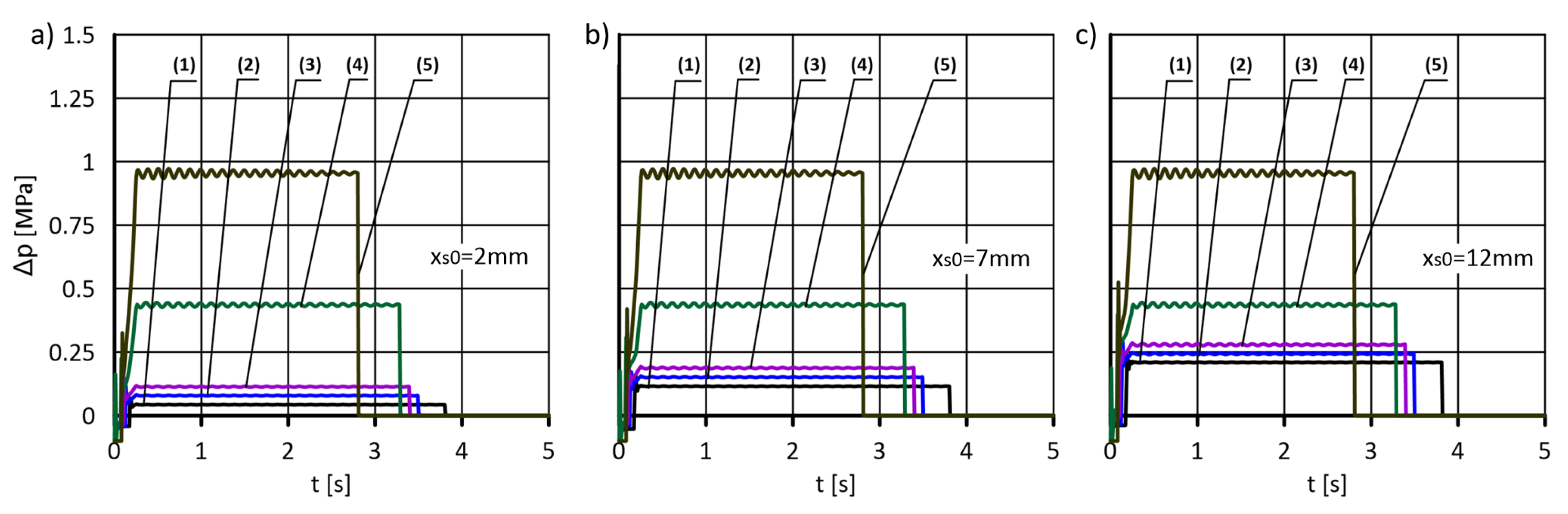
5.2. Determination of the Pressure Drop across the Valve

In the next stage, the value of the pressure drop on the check valve was determined as a function of the flow rate depending on the stiffness and initial spring tension. Figure 14 and Figure 15 and Table 5 show the pressure drop against time for different stiffness values in the A-B and B-A direction, respectively. Figure 16 and Figure 17 and Table 6 present the results obtained for the nominal spring with the different initial tension values. Depending on the flow rate and spring parameters, the obtained pressure drop varies from 0.25 MPa to 1.59 MPa in the A-B direction and from 0.08 MPa to 0.95 MPa in the B-A, respectively.

5.3. Estimation of the Check Valve Energy Efficiency

With the valve flow rate and pressure drop determined, the power required to open the valve and the total energy loss during the working cycle were estimated. The summary of the required power is shown in Figure 18, while the energy consumption is presented in Figure 19. As can be seen from the results, energy losses across the valve depend mainly on the flow rate and, to a lesser extent, on the spring stiffness. When operating at a nominal flow rate of Q = 300 dm3 min−1, the power requirements do not exceed 7 kW for the A-B flow direction and 3 kW for the opposite. This results in energy consumption during the working cycle of approximately 31 kJ and 12 kJ, respectively. Increasing the flow rate to 900 dm3 min−1 causes an over 4-fold increase in power demand, which leads to the energy consumption of the working cycle being 122 kJ (A-B) and 59 kJ (B-A).
The percentage share of energy consumed by the check valve and the effective cylinder piston displacement compared to the total energy necessary to complete the hydraulic system working cycle in both directions is presented in Table 7.
The obtained results show that the energy losses on the valve at nominal flow 300 dm3 min−1 do not exceed 3–5% of the total energy consumption during the flow in the A-B direction and 1–2% in the B-A direction, depending on the spring stiffness. Increasing the flow rate to 900 dm3 min−1 results in a greater percentage of valve loss; however, in the worst case, it is 7–8% and 5%, respectively. At the same time, the share of energy effectively used to move the actuator decreases from 92.3–94.3% to 85.6–88.3% for A-B and from 97.1–97.6% to 91.5% for B-A.

6. Comparison of Results with Laboratory Experiments

The last stage of the research was verifying the simulation results using the laboratory tests of the valve prototype provided by the manufacturer. Due to technical limitations, the bench tests were carried out for flow rates up to 350 dm3 min−1. A valve spring with a nominal rate of k s p r = 41.0 N mm−1 was used. The test bench scheme and the valve prototype during the tests are shown in Figure 20.
Each test consisted of the following steps: setting the minimum pump flow, opening the flow by overriding the control valve, and measuring the pressures while gradually increasing the pump flow to the maximum value and then back to zero. The pressures were measured with Trafag NAT sensors with a range of 32 MPa, an accuracy class of ± 0.2 % and voltage transducers 0–10 V. A Kracht TM turbine flow meter with a range of 2–500 dm3 min−1 and an accuracy class of ± 0.5 % and analogous voltage output signal was used to measure the flow rate. A 16-bit NI PCIe-6321 DAQ card with an SCB-68A terminal acquired pressure and flow rate signals from transducers. The measured pressure drop on the check valve was compared with the results of the numerical calculations, shown in Figure 21.
A high level of convergence of simulation and laboratory results was obtained. The value of the Pearson’s correlation coefficient determined for the A-B flow direction is R A B = 0.95 , while for B-A, it is R B A = 0.98 .

7. Summary and Conclusions

The subject of the analysis presented in this paper was a tunable check valve with a nominal flow Q = 300 dm3 min−1 and maximum working pressure p m a x = 35 MPa. As part of the research, CFD analyses and simulations in the Matlab/Simulink environment were carried out to obtain the flow characteristics of the valve. In particular, the values of the flow gap opening width and pressure drop were obtained as a function of the flow rate and the parameters of a spring pressing the valve plug against the seat, including spring stiffness and initial tension. A system with a one-sided hydraulic cylinder and a control valve was adopted to carry out the tests, ensuring the possibility of moving the piston rod in both directions. The hydraulic cylinder rod was loaded with the force F c y l = 500 kN, which ensured that the pressure in the system was close to the maximum value. Pressure drop and the related energy losses across the valve were estimated at the flow rates up to Q = 900 dm3 min−1. The simulation outcomes show a high level of compliance with the results of laboratory tests carried out on the valve prototype by the manufacturer.
The detailed conclusions are as follows:
  • The energy losses across the valve vary substantially depending on flow direction. Although the same connection diameters are used, the flow direction significantly impacts the amount of loss.
  • The spring stiffness and the initial tension, which is necessary to maintain tightness, are of significant importance for the level of energy loss, especially at lower flows. On the other hand, energy losses at the flow that guarantees full valve opening no longer depend on the spring parameters.
  • With the flow rate not exceeding the nominal value Q = 300 dm3 min−1, the determined energy losses are at the maximum level of 2–4% of the total system demand. However, the results show that the valve is not fully open. On the one hand, this makes the spring parameters more affecting the pressure drop, while on the other, it encourages research on expanding the flow rate range.
  • Doubled nominal flow Q = 600 dm3 min−1 causes the valve to open fully in the B-A direction and almost entirely in the A-B when using a softer spring. The share of energy losses, in this case, was 2.5% (B-A) and 4.1% (A-B), which can be considered acceptable values, as they are close to those obtained by a valve with a standard spring at nominal flow.
  • The maximum flow rate Q = 900 dm3 min−1 resulted in full opening in both directions. Depending on the flow direction, energy losses were estimated at 5.2–8.2%. These are not disqualifying values; however, taking into account the additional losses on the other components of the system, they should be included in the overall energy balance of the system.

Author Contributions

Conceptualization, E.L.; methodology, G.F. and J.R.; software, E.L. and G.F.; validation, J.R. and E.L.; formal analysis, J.R.; investigation, E.L., G.F. and J.R.; resources, J.R.; writing—original draft preparation, G.F.; writing—review and editing, E.L.; visualization, G.F.; supervision, E.L.; project administration, G.F.; funding acquisition, E.L. and G.F. All authors have read and agreed to the published version of the manuscript.

Funding

This research received no external funding.

Institutional Review Board Statement

Not applicable.

Informed Consent Statement

Not applicable.

Data Availability Statement

Not applicable.

Conflicts of Interest

The authors declare no conflict of interest.

Nomenclature

Indices
0 , 1 , 2 flow line
c v check valve
c y l hydraulic cylinder
ppoppet of the check valve
r e t return line
Parameters
A c y l , A c y l , r cylinder piston area, piston area on the rod side (m2)
A p A , A p B valve poppet left/right sectional area (m2)
A p C valve pilot sectional area (m2)
B f fluid bulk modulus (Pa)
C 1 ε , C 2 ε , C μ turbulence model constants (-)
E t o t a l total energy consumption per operating cycle (kJ)
F l o a d external force exerted on the hydraulic cylinder (N)
F h s , F h d , F s p r , F f force: hydrostatic, hydrodynamic, spring, friction (N)
I , turbulence model factors: intensity, length scale (-, m)
Q n o m nominal flow rate (dm3 min−1)
Q 0 , Q 1 , Q 2 Q r e t flow rate: pump, line 1, 2, return (dm3 min−1)
Ucontrol valve control signal (percentage) (%)
V 0 , V 1 , V 2 volume: supply line, line 1,2 (m3)
d p , l p , c r p , e p poppet dimensions: diameter, length, clearance, eccentricity (m)
k s p r valve spring stiffness (N m−1)
m p , m p 2 , m c y l mass: valve poppet, valve pilot, cylinder piston with rod (kg)
p 0 , p 1 , p 2 , p r e t pressure: supply line, 1, 2, return line (MPa)
Δ p pressure drop (MPa)
q r e v pump piston stroke rate per revolution (m3/rev)
s k , s ε turbulence model constants (-)
t , t s t a r t time, start-up time (s)
v p , v c y l , v a v g velocity: poppet, cylinder piston, fluid (average) (m s−1)
x p , x c y l position: valve poppet, hydraulic cylinder piston (m)
x s 0 initial valve spring deflection (m)
znumber of pistons (pump) (-)
α poppet head opening angle (°)
η fluid dynamic viscosity (Pa s)
λ check valve jet angle coefficient (-)
ν fluid kinematic viscosity (m2 s−1)
μ t turbulent viscosity (m2 s−1)
ρ fluid density (kg m−3)
φ damping coefficient (N s m−1)
Φ g valve poppet friction force geometrical factor (m)
ω 0 , ω n o m pump rotational speed, pump nominal speed (rev/s)

References

  1. Ye, J.; Zhao, Z.; Zheng, J.; Salem, S.; Yu, J.; Cui, J.; Jiao, X. Transient Flow Characteristic of High-Pressure Hydrogen Gas in Check Valve during the Opening Process. Energies 2020, 13, 4222. [Google Scholar] [CrossRef]
  2. Ye, J.; Zhao, Z.; Cui, J.; Hua, Z.; Peng, W.; Jiang, P. Transient flow behaviors of the check valve with different spool-head angle in high-pressure hydrogen storage systems. J. Energy Storage 2022, 46, 103761. [Google Scholar] [CrossRef]
  3. Kim, N.S.; Jeong, Y.H. An investigation of pressure build-up effects due to check valve’s closing characteristics using dynamic mesh techniques of CFD. Ann. Nucl. Energy 2021, 152, 107996. [Google Scholar] [CrossRef]
  4. Wen, Q.; Liu, Y.; Chen, Z.; Wang, W. Numerical simulation and experimental validation of flow characteristics for a butterfly check valve in small modular reactor. Nucl. Eng. Des. 2022, 391, 111732. [Google Scholar] [CrossRef]
  5. Lai, Z.; Karney, B.; Yang, S.; Wu, D.; Zhang, F. Transient performance of a dual disc check valve during the opening period. Ann. Nucl. Energy 2017, 101, 15–22. [Google Scholar] [CrossRef]
  6. Gomez, I.; Gonzalez-Mancera, A.; Newell, B.; Garcia-Bravo, J. Analysis of the Design of a Poppet Valve by Transitory Simulation. Energies 2019, 12, 889. [Google Scholar] [CrossRef] [Green Version]
  7. Deng, H.; Liu, Y.; Li, P.; Ma, Y.; Zhang, S. Integrated probabilistic modeling method for transient opening height prediction of check valves in oil-gas multiphase pumps. Adv. Eng. Softw. 2018, 118, 18–26. [Google Scholar] [CrossRef]
  8. Ling, M.; He, X.; Wu, M.; Cao, L. Dynamic Design of a Novel High-Speed Piezoelectric Flow Control Valve Based on Compliant Mechanism. IEEE/ASME Trans. Mechatron. 2022, 1–9. [Google Scholar] [CrossRef]
  9. Shin, S.M.; Kim, D.S.; Kang, H.G. Power-operated check valve in abnormal situations. Nucl. Eng. Des. 2018, 330, 28–35. [Google Scholar] [CrossRef]
  10. Morgan, S.C.; Hendricks, A.D.; Seto, M.L.; Sieben, V.J. A Magnetically Tunable Check Valve Applied to a Lab-on-Chip Nitrite Sensor. Sensors 2019, 19, 4619. [Google Scholar] [CrossRef] [Green Version]
  11. Gao, Z.x.; Liu, P.; Yue, Y.; Li, J.y.; Wu, H. Comparison of Swing and Tilting Check Valves Flowing Compressible Fluids. Micromachines 2020, 11, 758. [Google Scholar] [CrossRef] [PubMed]
  12. Baluyev, D.; Gusev, D.; Meshkov, S.; Nikanorov, O.; Osipov, S.; Rogozhkin, S.; Rukhlin, S.; Shepelev, S. Study of functional characteristics for safety system check valve using scaled model. Nucl. Energy Technol. 2015, 1, 99–102. [Google Scholar] [CrossRef] [Green Version]
  13. Yang, L.J.; Waikhom, R.; Wang, W.C.; Jabaraj Joseph, V.; Esakki, B.; Kumar Unnam, N.; Li, X.H.; Lee, C.Y. Check-Valve Design in Enhancing Aerodynamic Performance of Flapping Wings. Appl. Sci. 2021, 11, 3416. [Google Scholar] [CrossRef]
  14. Schickhofer, L.; Wimmer, J. Fluid–structure interaction and dynamic stability of shock absorber check valves. J. Fluids Struct. 2022, 110, 103536. [Google Scholar] [CrossRef]
  15. Filo, G.; Lisowski, E.; Rajda, J. Pressure Loss Reduction in an Innovative Directional Poppet Control Valve. Energies 2020, 13, 3149. [Google Scholar] [CrossRef]
  16. Filo, G.; Lisowski, E.; Rajda, J. Design and Flow Analysis of an Adjustable Check Valve by Means of CFD Method. Energies 2021, 14, 2237. [Google Scholar] [CrossRef]
  17. Novak, P.; Guinot, V.; Jeffrey, A.; Reeve, D.E. Hydraulic Modelling—An Introduction: Principles, Methods and Applications; CRC Press, Taylor & Francis Group: Boca Raton, FL, USA, 2010. [Google Scholar]
  18. Lisowski, E.; Filo, G. CFD analysis of the characteristics of a proportional flow control valve with an innovative opening shape. Energy Convers. Manag. 2016, 123, 15–28. [Google Scholar] [CrossRef]
  19. Valdés, J.R.; Miana, M.J.; Núñez, J.L.; Pütz, T. Reduced order model for estimation of fluid flow and flow forces in hydraulic proportional valves. Energy Convers. Manag. 2008, 49, 1517–1529. [Google Scholar] [CrossRef]
  20. Posa, A.; Oresta, P.; Lippolis, A. Analysis of a directional hydraulic valve by a Direct Numerical Simulation using an immersed-boundary method. Energy Convers. Manag. 2013, 65, 497–506. [Google Scholar] [CrossRef]
  21. Lisowski, E.; Filo, G.; Rajda, J. Pressure compensation using flow forces in a multi-section proportional directional control valve. Energy Convers. Manag. 2015, 103, 1052–1064. [Google Scholar] [CrossRef]
  22. Anh, P.N.; Bae, J.S.; Hwang, J.H. Computational Fluid Dynamic Analysis of Flow Rate Performance of a Small Piezoelectric-Hydraulic Pump. Appl. Sci. 2021, 11, 4888. [Google Scholar] [CrossRef]
  23. Woldemariam, E.T.; Lemu, H.G.; Wang, G.G. CFD-Driven Valve Shape Optimization for Performance Improvement of a Micro Cross-Flow Turbine. Energies 2018, 11, 248. [Google Scholar] [CrossRef] [Green Version]
  24. Chen, F.; Qian, J.; Chen, M.; Zhang, M.; Chen, L.; Jin, Z. Turbulent compressible flow analysis on multi-stage high pressure reducing valve. Flow Meas. Instrum. 2018, 61, 26–37. [Google Scholar] [CrossRef]
  25. Jin-yuan, Q.; Lin, W.; Zhi-jiang, J.; Jian-kai, W.; Han, Z.; An-le, L. CFD analysis on the dynamic flow characteristics of the pilot-control globe valve. Energy Convers. Manag. 2014, 87, 220–226. [Google Scholar] [CrossRef]
  26. Scuro, N.; Angelo, E.; Angelo, G.; Andrade, D. A CFD analysis of the flow dynamics of a directly-operated safety relief valve. Nucl. Eng. Des. 2018, 328, 321–332. [Google Scholar] [CrossRef]
  27. ANSYS Fluent Tutorial Guide, 18.0 ed.; ANSYS Inc.: Canonsburg, PA, USA, 2017; Available online: http://www.ansys.com (accessed on 6 June 2022).
  28. ISO:4411:2019; Hydraulic Fluid Power—Valves—Determination of Differential Pressure/Flow Rate Characteristics. ISO: Geneva, Switzerland, 2019.
Figure 1. Scheme of the analyzed tunable check valve: 1—body, 2, 3—cover, 4—poppet, 5—ball, 6—disc, 7—spring, 8—pilot spool; A,B—connection ports.
Energies 15 05740 g001
Figure 2. Scheme of hydraulic system: 1—pump, 2—relief valve, 3—control valve, 4—check valve, 5—actuator; (A-B), (B-A)—flow directions.
Energies 15 05740 g002
Figure 3. Balance of forces acting on the check valve poppet; (a) A-B flow direction, (b) B-A flow direction.
Energies 15 05740 g003
Figure 4. Mesh model with refined areas marked: (a) initial, (b) dense, refined poppet head and seat, (c) double dense, refined; A,B—connection ports.
Energies 15 05740 g004
Figure 5. Results of CFD simulation for poppet position x p = 1.0 mm: (a) pressure distribution, (b) velocity distribution; λ = 67 . 8 .
Energies 15 05740 g005
Figure 6. Results of CFD simulation for poppet position x p = 3.0 mm: (a) pressure distribution, (b) velocity distribution; λ = 62 . 1 .
Energies 15 05740 g006
Figure 7. Results of CFD simulation for poppet position x p = 5.0 mm: (a) pressure distribution, (b) velocity distribution; λ = 56 . 0 .
Energies 15 05740 g007
Figure 8. Simulation model for the A-B flow direction.
Energies 15 05740 g008
Figure 9. Difference in the simulation model for the B-A flow direction.
Energies 15 05740 g009
Figure 10. Piston pump flow rate with an average value of: 100 ( 1 ) , 200 ( 2 ) , 300 ( 3 ) , 600 ( 4 ) , and 900 ( 5 ) dm3 min−1.
Energies 15 05740 g010
Figure 11. Check valve gap width x p ( t ) and hydraulic actuator displacement c c y l ( t ) for the nominal stiffness k s p r = k n o m = 41.0 N mm−1; (a) A-B flow direction, (b) B-A flow direction.
Energies 15 05740 g011
Figure 12. Check valve gap width x p ( t ) and hydraulic actuator displacement c c y l ( t ) for the reduced stiffness k s p r = k 1 = 24.6 N mm−1; (a) A-B flow direction, (b) B-A flow direction.
Energies 15 05740 g012
Figure 13. Check valve gap width x p ( t ) and hydraulic actuator displacement c c y l ( t ) for the increased stiffness k s p r = k 2 = 57.4 N mm−1; (a) A-B flow direction, (b) B-A flow direction.
Energies 15 05740 g013
Figure 14. Pressure drop on check valve for different spring rates: (a) reduced, (b) nominal, (c) increased; flow direction A-B.
Energies 15 05740 g014
Figure 15. Pressure drop on check valve for different spring rates: (a) reduced, (b) nominal, (c) increased; flow direction B-A.
Energies 15 05740 g015
Figure 16. Pressure drop on check valve for different initial spring tension values: (a) reduced, (b) nominal, (c) increased; flow direction A-B.
Energies 15 05740 g016
Figure 17. Pressure drop on check valve for different initial spring tension values: (a) reduced, (b) nominal, (c) increased; flow direction B-A.
Energies 15 05740 g017
Figure 18. The power required to open the valve, flow direction: (a) A-B, (b) B-A.
Energies 15 05740 g018
Figure 19. Energy consumption of the valve during the working cycle, flow direction: (a) A-B, (b) B-A.
Energies 15 05740 g019
Figure 20. Test bench: (a) scheme, (b) valve; 1—pump, 2—relief valve, 3—tested check valve, 4—control valve, 5—throttle valve, 6—filter, 7—flow meter, 8—temperature gauge, 9,10—pressure transducers, 11—computer DAQ system.
Energies 15 05740 g020
Figure 21. Comparison of the pressure drop on the check valve from numerical simulations and laboratory tests as a function of flow rate; vertical markers—standard deviation.
Energies 15 05740 g021
Table 1. Physical model parameters.
Kinematic ViscosityDensityTemperatureMin Inlet FLOW RateMax Inlet Flow RateOutlet Pressure
ν ρ T Q m i n Q m a x p r e t
41 × 10 6 87050.01009000.1
m2 s−1kg m−3°Cdm3 min−1dm3 min−1MPa
Table 2. Turbulence model parameters.
Kinetic Energy
Constant
Kinetic Energy
Dissipation Constants
Turbulent Viscosity
Constant
Turbulence IntensityLength Scale
s k s ε C 1 ε C 2 ε C μ I
1.01.31.441.920.094.5–5.91.53
-----%mm
Table 3. Mesh quality assessment.
Mesh CaseNo. of NodesNo. of ElementsComput. TimePressure DropDifference from
Laboratory Result
Initial (I) 3.0 × 10 3 1.3 × 10 4 30 min 0.566 MPa 14.21 %
Dense,
refined (II)
9.1 × 10 4 4.6 × 10 5 240 min 0.644 MPa 2.36 %
Double dense,
refined (III)
2.5 × 10 5 1.4 × 10 6 1660 min 0.645 MPa 2.32 %
Table 4. Jet angle against poppet position from CFD simulation.
InputQ (dm3 min−1)300
x p (mm)1.02.03.04.05.0
Output λ ( )67.865.062.158.956.0
Table 5. Check valve pressure drop (MPa) against flow rate Q and spring stiffness k s p r .
x s 0
mm
Q
dm3 min−1
k spr = 24.6 N/mm k spr = 41.0 N/mm k spr = 57.4 N/mm
A-BB-AA-BB-AA-BB-A
7.01000.340.060.480.120.650.17
2000.410.100.560.150.740.21
3000.470.150.650.190.830.25
6000.700.390.920.421.150.43
9001.260.891.370.921.510.92
Table 6. Check valve pressure drop (MPa) against flow rate Q and initial tension x s 0 .
k spr
N/mm
Q
dm3 min−1
x s 0 = 2.0 mm x s 0 = 7.0 mm x s 0 = 12.0 mm
A-BB-AA-BB-AA-BB-A
41.01000.240.050.480.120.770.21
2000.320.080.560.150.850.24
3000.410.110.650.190.930.26
6000.670.390.920.421.210.43
9001.260.901.370.921.560.92
Table 7. Percentage share of energy consumption by the check valve E c v and the hydraulic cylinder E c y l against flow rate Q and spring stiffness k s p r .
DirectionQ
dm3 min−1
k spr = 24.6 N/mm k spr = 41.0 N/mm k spr = 57.4 N/mm
E cv % E cyl % E cv % E cyl % E cv % E cyl %
A-B1002.195.42.994.63.893.7
2002.495.13.494.24.393.2
3002.894.33.893.34.992.3
6004.191.55.290.46.489.3
9007.088.37.086.78.285.6
B-A1000.998.11.297.91.697.7
2000.898.01.297.71.597.5
3000.997.61.397.31.797.1
6002.595.52.595.52.695.4
9005.291.55.291.55.291.5
Publisher’s Note: MDPI stays neutral with regard to jurisdictional claims in published maps and institutional affiliations.

