Article

FTCN: A Reservoir Parameter Prediction Method Based on a Fusional Temporal Convolutional Network

1
Qingdao Institute of Software, College of Computer Science and Technology, Qingdao 266580, China
2
School of Geosciences, China University of Petroleum (East China), Qingdao 266580, China
3
Geophysical Research Institute of Shengli Oilfeld Branch, Sinopec, Dongying 257022, China
4
Shandong Provincial Key Laboratory of Deep Oil & Gas, China University of Petroleum (East China), Qingdao 266580, China
*
Author to whom correspondence should be addressed.
Energies 2022, 15(15), 5680; https://doi.org/10.3390/en15155680
Submission received: 14 July 2022 / Revised: 31 July 2022 / Accepted: 2 August 2022 / Published: 5 August 2022

Abstract

:
Predicting reservoir parameters accurately is of great significance in petroleum exploration and development. In this paper, we propose a reservoir parameter prediction method named a fusional temporal convolutional network (FTCN). Specifically, we first analyze the relationship between logging curves and reservoir parameters. Then, we build a temporal convolutional network and design a fusion module to improve the prediction results in curve inflection points, which integrates characteristics of the shallow convolution layer and the deep temporal convolution network. Finally, we conduct experiments on real logging datasets. The results indicate that compared with the baseline method, the mean square errors of FTCN are reduced by 0.23, 0.24 and 0.25 in predicting porosity, permeability, and water saturation, respectively, which shows that our method is more consistent with the actual reservoir geological conditions. Our innovation is that we propose a new reservoir parameter prediction method and introduce the fusion module in the model innovatively. Our main contribution is that this method can well predict reservoir parameters even when there are great changes in formation properties. Our research work can provide a reference for reservoir analysis, which is conducive to logging interpreters’ efforts to analyze rock strata and identify oil and gas resources.

1. Introduction

Reservoir parameters are very important in petroleum exploration and development and also a significant reference foundation to analyze reservoir geology and evaluate oil and gas reservoirs accurately. In the actual exploitation process, obtaining reservoir parameters is expensive from core data, and the amount of data obtained is limited. At the same time, the actual development environment is changeable, and the underground geological situation is complex and diverse. Affected by the original data, logging cost, the level of explorers, the empirical coefficients, response logging curve selection, heterogeneous formation, depositional environment and tectonic location, it becomes extremely complex to obtain accurate reservoir parameters.
In recent years, artificial intelligence technology has provided a possibility for intelligent exploration [1]. Deep learning methods such as BP (back propagation) network [2], recurrent neural network (RNN) [3], long short-term memory (LSTM) [4] and gated recurrent unit (GRU) [5] have been applied to petroleum field by many researchers. Dos [6] proposed a computational system based on deep recurrent neural networks (RNNs) as an effective method to automatically identify lithofacies patterns from well logs. For forecasting petroleum production, a novel method based on a gated recurrent neural network has been proposed. It has multiple hidden layers, and each layer has a number of nodes. The robustness of this model is very good [7]. Heghedus [8] concentrated on pressure-rate datasets accumulated with massive installation of permanent downhole gauge production and injection wells based on an LSTM network. The research results provide a basis for filling gaps in well monitoring data. Meanwhile, it also becomes a research hotspot for intelligent reservoir parameter prediction.
For the sake of enhancing the prediction results of reservoirs in intricate geology effectively, a new parameter prediction method named the fusional temporal convolutional network (FTCN) has been proposed. Firstly, the relationship between logging curves and reservoir parameters is analyzed deeply, and the logging curves, which are closely related to reservoir parameters, are obtained. We use the selected correlation logging curves to predict the reservoir parameters. Secondly, we present a fusion module on TCN to improve the affection of reservoir parameter prediction innovatively. We weigh the output of different network layers and combine the output to enrich the data characteristics obtained by the predictive network model. A fusion module is raised to utilize the information from different network layers adequately, which decreases the large deviation in the fluctuation of local peak values. Finally, experiments are set up on the actual logging data. Our method provides better support to understand and analyze reservoir conditions technically and thus provides a novel reference to the exact interpretation of the logging data.
There are a lot of measurement data in the petroleum industry. These data usually contain momentous information describing the characteristics of strata and reservoir properties and play an important role in production and reservoir management. Logging records provide a data source for logging interpretation experts to analyze reservoir properties. Logging experts can obtain the information of reservoir characteristics by analyzing logging records. Reservoir parameters are exceedingly significant for logging interpreters to analyze formation properties and reservoir capacity and are also the foundation for fine logging reservoir evaluation and analysis of oil-gas. Reservoir parameters, such as porosity, permeability and water saturation, reflect the reservoir’s storing ability. Generally, the greater the porosity is, the more likely it is to store oil and natural gas in the pores. The higher the permeability is, the stronger the fluidity of oil, and the easier it is to be exploited. Predicting reservoir parameters effectively can provide a reference for analyzing reservoir properties, characterizing oil reservoirs and providing accurate interpretation of well logging data, which can assist logging interpreters in judging formation conditions and evaluating oil-gas potential. Thus, it provides a support for reserve calculation, flow unit identification and reservoir evaluation. Using the effective porosity parameter of the fracture and cavity reservoirs in combination with the effective thickness, oil-bearing area and other reserve calculation parameters, Kuanzhi [9] formulated a reserve estimation scheme for fractured vuggy carbonate reservoirs so as to guide the exploration and development of oil and gas reservoirs. In the research of reservoir flow unit identification in the North Rumaila Oilfield, according to the logging curve similarity, the porosity and permeability crossplot, the capillary pressure data, the porosity and water saturation and depth relationship and the flow zone indication method, Al-Jawad [10] subdivided the primary reservoir units in the oilfield, interpreted and classified the sub units and thus identified the good reservoirs. Therefore, reservoir parameters play an important role in the exploration and development of the petroleum industry.
The main contributions of this paper are as follows:
(1)
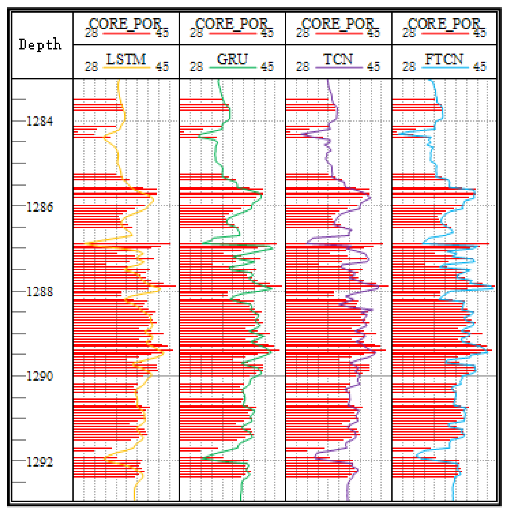
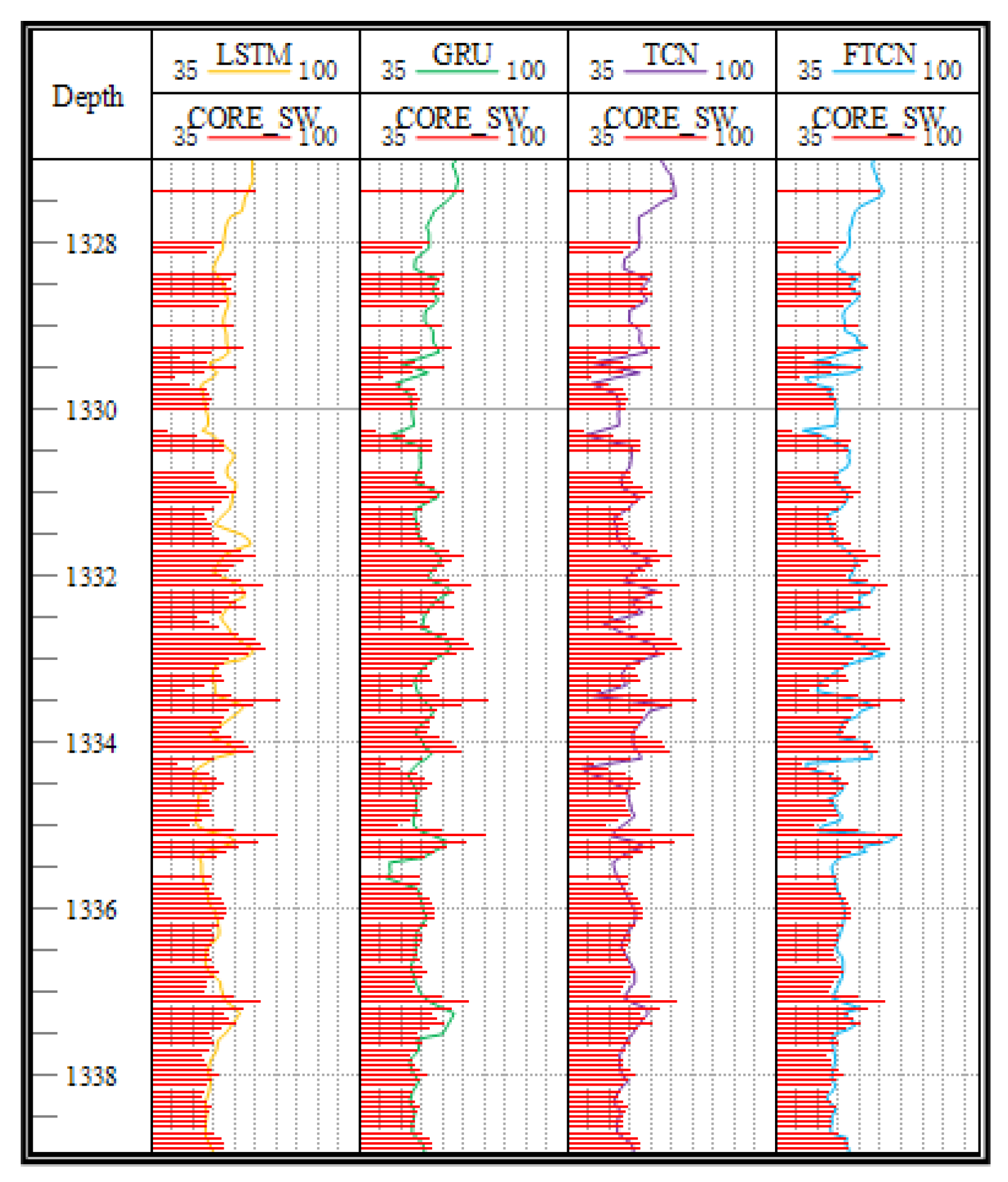
Our method can predict reservoir porosity, permeability and water saturation effectively. It is beneficial for logging interpreters to analyze rock strata and identify oil and gas resources;
(2)
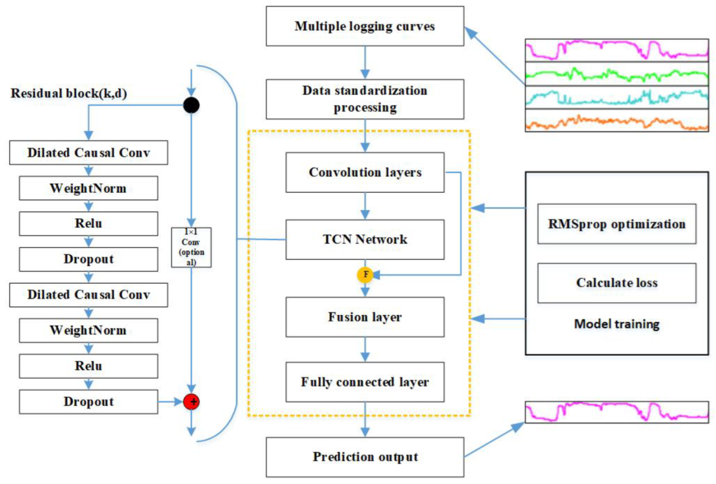
A new reservoir parameter prediction method named FTCN is proposed. We introduce a fusion module based on TCN to utilize the information from different network layers adequately, which improves the effect of curve prediction;
(3)
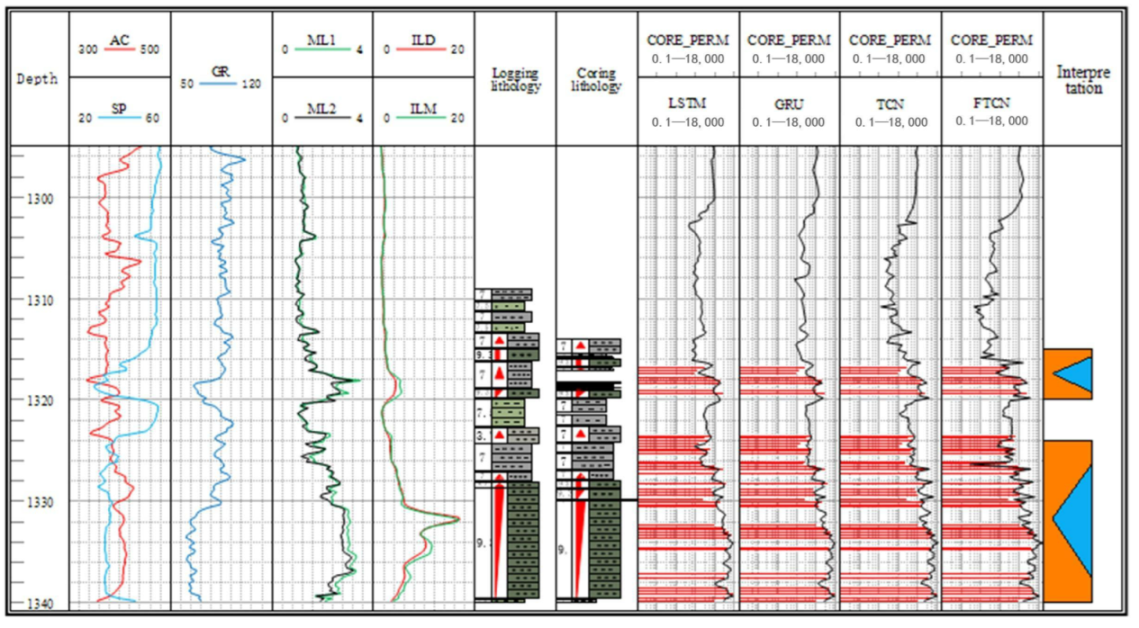
We have conducted various experiments on the real logging dataset to illustrate the effectiveness of this method. FTCN can predict well where the log curve changes abruptly and is effective when the properties of underground strata change greatly.

2. Previous Work

Complex reservoir analysis is a significant field in oil reservoir description. Well logging data involves abundant geological information. By analyzing logging data, logging interpreters can judge stratum properties and identify oil and gas reservoirs. In recent years, with the incessant development of machine learning, there have been many outstanding works in the field of engineering applications of deep learning or convolutional networks. For example, a novel method based on deep convolutional neural networks to identify and localise damages to building structures equipped with smart control devices has been proposed [11]. In addition, Yu [12] developed a vision-based crack diagnosis method using a deep convolutional neural network (DCNN) and enhanced chicken swarm algorithm (ECSA). It has also been applied in the domain of petroleum logging successfully [13]. Scholars have done a great deal of research and achieved many achievements in the integration of oil exploration and development and artificial intelligence [14]. For example, the porosity classification and quantification scheme [15] mainly introduces a thorough understanding of the carbonate pore system, which is essential to hydrocarbon prospecting and the prediction of petroleum reservoir properties [16]. Other examples include sedimentary facies classification, reservoir evaluation [17], and so on.
A variety of methods have been proposed to solve the problem of reservoir parameter prediction, which continuously promotes the development of reservoir analysis and logging interpretation technology and provides an important basis for geological experts to analyze reservoirs. In the early stage, based on years of experience in the analysis of reservoir parameters and geological conditions, researchers [18,19,20] established many empirical formulas to determine the reservoir parameters in the research field. However, because the geological conditions of the new and old exploration areas are different, there will be great differences. A new, undeveloped study area is likely to have rich potential oil and gas resources and good reservoir physical properties. However, in an old study area, due to long-term development, the physical properties and lithology of the reservoir will have changed, and the geological conditions become very poor, which brings challenges to the development of the remaining oil and gas resources. Some empirical coefficient values cannot be generalized, and the formula is also affected by the subjective factors of logging interpreters. Thus, the results are uncertain. Empirical formulas can only be used as a reference. In addition, cross plots can also be used to analyze reservoir properties in exploration and development [21]. The cross plot draws a two-factor or multi-factor rendezvous map using logging curve readings or calculation parameters. Geological experts interpret geological models and analyze and evaluate strata according to the observation of cross plots, which is also uncertain. Therefore, the above methods are influenced by the subjective factors of logging interpreters and the great changes in geological conditions, so the accuracy of the reservoir parameter prediction needs to be improved.
As mature oilfields turn into a later exploitation period of the ultra-high water cut stage, the geological situation becomes complex and changeable, and the quality of oil resources gradually deteriorates [22]. The search for oil and gas fields with complex reservoirs has become difficult, and traditional methods have been unable to meet the demand. The development of machine learning technology makes it possible to improve the effect of reservoir parameter prediction [23].
Through the analysis of tight sandstone reservoirs, Zhu [24] considered that the clay content, the irreducible water saturation, the porosity and the diagenetic coefficient were important factors affecting the reservoir parameter permeability. The studied samples of the model were selected based on the representative core analysis data. According to these influencing factors and samples, permeability was predicted based on an improved BP neural network. Mahdaviara [25] pointed out that the prediction of permeability was a challenge in carbonate heterogeneous rock and built a model to predict reservoir permeability based on Gaussian process regression. The evaluation of permeability in the southern Yellow Sea basin showed that it can be used as a supplement to the neural network prediction methods. In addition, researchers [26,27] have used machine learning methods, such as support-vector machines, particle swarm optimization algorithm [28], and artificial neural networks [29,30,31] to study and analyze reservoir parameters, achieving good results.
As a research hotspot in the domain of machine learning, deep learning has achieved fruitful results in many fields, such as agriculture [32], ultrasound imaging [33], smart cities [34] and so on. Many researchers have applied deep learning to the field of petroleum exploration and development [35,36]. In the study of predicting reservoir parameters, deep learning technology has been combined to improve the prediction accuracy. As two significant parameters of the oil and gas storage, porosity and shale content express the sedimentary characteristics of various historical stages and have an intense nonlinear mapping with logging parameters. Deep learning has a powerful data mining capacity. Therefore, AN [37] applied an LSTM network to predict the shale content and porosity of a reservoir. The prediction accuracy of this network was more superior than the conventional deep neural network. The hardship of gaining porosity increases gradually with increasing drilling depth, and the cost for gaining intact porosity by the conventional coring method is large comparatively. Thus, for the sake of achieving low-cost and high-efficiency porosity prediction, Chen [38] proposed a logging method found on a multi-layer LSTM network, which performs well for logging at different depths and predicts the changing trend of porosity in strata effectively. The logging curves gained from deep to shallow stratum indicate the sedimentary features of distinct geological stages. The porosity, as a vital reservoir parameter, reflects the capacity of the oil and gas storage. It is very meaningful for the exact description of a reservoir to use logging parameters to acquire reservoir porosity [39]. The application effect in a certain research region of the Ordos basin showed that a gated recurrent unit (GRU) network combined with various logging curves was more effective in predicting reservoir porosity than multiple regression analysis as well as RNN. In addition, convolution structures [40,41] also have certain advantages in predicting sequence tasks. However, although the above methods solve the problem of reservoir parameter prediction in some practical areas effectively, the effect on geological complex reservoir prediction is general, such as in an old oilfield with serious water flooding and intense inhomogeneity. The structure of the reservoir sand body is loose, and the lithology is complex. Development is difficult, and the effect needs to be further improved. The generalization of the model is limited to a certain extent, so these methods have some limitations in practical application and cannot meet the requirements of all kinds of fine reservoir prediction.

3. Methodology

LSTM [4] was first proposed by Hochreiter and Schmidhuber to solve the long-term dependence problem of general RNN, which can avoid gradient vanishing and gradient exploding. GRU [5] is an important variant of LSTM. It improves the design of gates in LSTM and optimizes the forgetting gate, input gate and output gate in LSTM into two gates called the reset gate and update gate, respectively. A temporal convolutional network (TCN) [40] is a special convolution network that has the advantages of a flexible receptive field and stable gradient.

3.1. FTCN Network Model

For the purpose of resolving problems of the resulting uncertainty, reservoir area limitation and low prediction accuracy, a fusional temporal convolutional network (FTCN) based on TCN is proposed in this paper by digging into the nonlinear relationship between logging curves and reservoir parameters in complex reservoirs. Firstly, the input curves are optimized by selecting the logging curves, which are sensitive to porosity, permeability and water saturation, and excluding the non-correlation curves. Then, a fusion module is designed to improve the prediction results of the inflection point of the curve, which can reduce the local deviation of reservoir parameter prediction parameters efficiently. The framework of FTCN is shown in Figure 1. A variety of logging curves are preprocessed. The middle part is the main structure of the prediction network. The right part shows the optimization of the network. Specifically, the original logging data mainly include acoustic travel time, density, compensated neutron logging, natural gamma ray, spontaneous potential, micro-potential resistivity, micro-gradient resistivity, and so on. We use the numerical values of these logging curves as the input data of the network model.
There are great differences in the value range of different logging curve data. For the sake of reducing the effect of different dimensions of the original logging data, the data are standardized and preprocessed as
y i j = x i j μ i s i ,
where i is the ith kind of curve parameter, j is the jth sample of the curve parameter, x i j denotes the original data, y i j denotes the standardized data, and μ i and s i are the mean and standard deviation of data, respectively.
The standardized data are used as the input data of the predictive network model and first enter the convolution layers, where convolution and pooling operations are carried out, which are mainly used to obtain the low-level features of the network. Then, they enter the TCN network, including dilated causal convolution and residual connection blocks, and the deep-level features of the data are obtained through the TCN network. Then, they enter the fusional module. After passing the network fusional module and then going through the full connection layer, the predicted reservoir parameters are output. In the process of adjusting the training network, we chose the RMSProp algorithm [42] with adaptive learning rate. Through continuous iterative training, the reservoir parameter prediction model is established.

3.2. Fusional Module
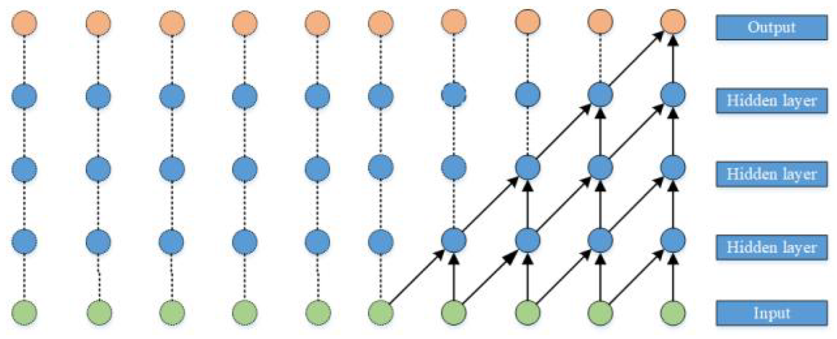
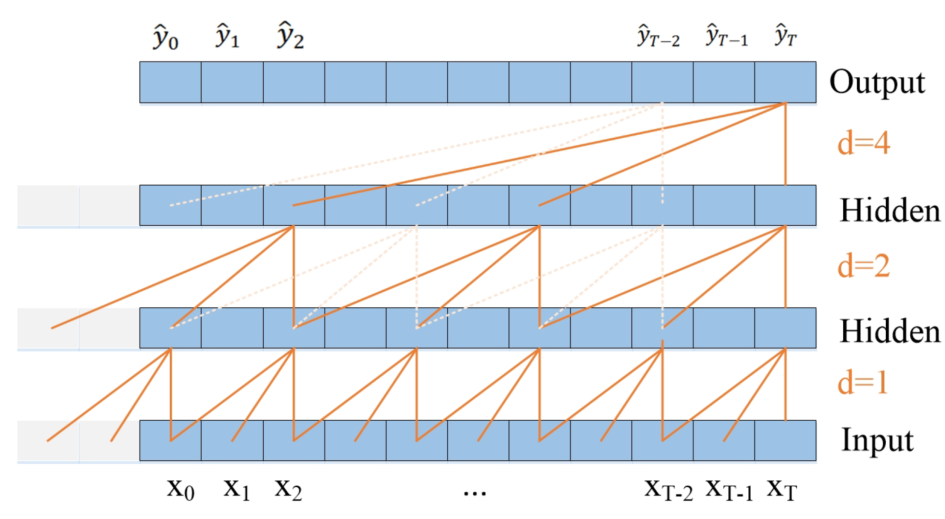
The variation of well logging curves reflects the change in reservoir parameters in some ways, and it has a good correlation among adjacent wells in the same horizon. Convolution networks have strong data mining abilities. Dilated convolution expands the receptive field by introducing a dilation factor to the convolution. This dilation factor defines the distance between values when the network processes data. The dilated convolution obtains the information farther from the current input by skipping part of the input value. In order to make the network remember more effective information, we introduce dilated convolution that can expand the receptive field into our network. Thus, the network can pay more attention to global information and capture more feature information. However, with the increase in network depth, dilated convolution will lose the continuity of data information and weaken the attention to local information. To get the most out of the non-linear mapping relation between logging curves and reservoir parameters, we combine the output weighting of shallow convolution layer and deep TCN network to enrich the data information obtained by prediction network model, and a network fusional module is designed as
F ( x ) = 1 + α 2 * T ( x ) * C ( x ) α 2 * T ( x ) + C ( x ) ,
where F ( x ) is the output of the fusion module, C ( x ) and T ( x ) are the output of the convolution layer and after the TCN, and  α is a balance factor, which is used to weigh the integration with the network layer.
This design considers the information of the deep and shallow network to enhance the prediction performance of the network comprehensively and maximize the characteristic information of the logging curves.

3.3. TCN Network

The network uses causal convolution to handle time series data. There is a causal relationship between different layers of the network, so that it does not have information leakage from the future into the past, as shown in Figure 2. At time t, the output is only convolved with t and earlier elements in an anterior layer. In order to make the network produce the same output as the input length, a one-dimensional fully convolutional network structure is used for TCN, in which the length of the hidden layer is the same as the input layer. In addition, it adds zero padding of kernel size 1 length to ensure that the length of the subsequent layer is equal to the preceding layers [40].
An ordinary causal convolution can merely review a history of linear size in the depth of the network, which results in difficulties when using causal convolution in assignments that require longer history. In order to remember long effective historical information, dilated convolution [43] is introduced into the network, which increases the receptive field of the kernel and maintains the parameters unchanged. Specifically, for a filter f : { 0 , , k 1 } R , a 1-D sequence input X R n , and sequence element e, the dilated convolution operational express F is denoted as
F ( e ) = X * d f ( e ) = i = 0 k = 1 f ( i ) · X e d · i ,
where d denotes the dilation factor. k denotes the filter size, and e d · i indicates the direction of the past. Therefore, the dilation corresponds to bringing in a fixed step in the middle of every two contiguous filter taps. When the d value is 1, dilated convolution turns into regular convolution. This utilization of greater dilation makes the top-level output express a broader input scope. Therefore, the receptive field in ConvNet is expanded effectively.
Dilated convolution obtains the information farther from the current input by skipping part of the input values. The dilation factor d( d = O 2 i ) increases along with the depth of network exponentially. This is  shown in Figure 3, which represents a dilated convolution when the filter size k = 3 and dilated factors d = 1 , 2 , 4 . Therefore, with the increase in the network layer, the receptive field of the network continues to increase, thus ensuring that the network can remember more historical information while avoiding an excessively deep network.
In general, the expression ability of neural networks increases with the increase in network depth, but a deeper and larger network can easily produce exploding gradients, vanishing gradients and so on. Residual connections are used in this network [44].
o = Activation ( x + F ( x ) ) ,
The residual block consists of a branch that leads to a train of transformations F ( x ) , and its output is appended to input x of this block, which avoids the degradation of very deep networks. The left part of the FTCN framework shows the residual block, which contains two dilated causal convolution layers, weight normalization layers and rectified linear unit layers. The dropout is used to discard some neurons to prevent overfitting. In addition, 1 × 1 convolution is applied to assure the element-wise addition ⊕ takes over tensors which have an identical shape. This design can retain information as much as possible and improve the performance of the network model.

3.4. FTCN Network Flow

The RMSProp algorithm is an effective and practical depth network optimization algorithm. It adjusts changes in the learning rate by combining an exponential moving average of the square of the gradient and can converge well in the case of the unstable objective function. According to the mean absolute error loss calculated by the prediction network model, the algorithm updates the model parameters by computing the gradient of each weight to optimize the network. The pseudo-code of the FTCN algorithm flow is shown in Algorithm 1, in which AC, CNL, DEN, GR and SP represent acoustic travel time, compensated neutron logging, density, natural gamma ray and spontaneous potential, respectively, and POR, PERM and SW represent porosity, permeability and water saturation, respectively.
Algorithm 1: FTCN RP = FTCN(LCS).
Energies 15 05680 i001

4. Results and Discussion

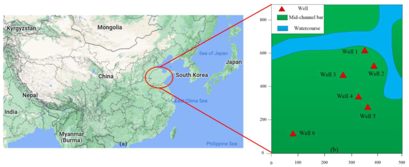
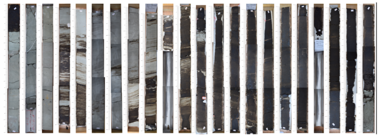
4.1. Geological Setting and Data Source

As shown in Figure 4, the experiment was set up on a real oil field reservoir, which is located in the east China. The Figure shows the relative position of the well. In this area, the braided river deposit is composed of a mid-channel bar and watercourse. The existence of different configuration units leads to the diversity and complexity of reservoir properties and development characteristics. In turn, the differences in reservoir properties and development characteristics also reflect the differences in sedimentary facies distribution or geological flow unit distribution. The oil field has entered the mid-to-late stage of development, and it is in the stage of high and ultra-high water cut. After long-term water flooding, the heterogeneity has become stronger, and the physical properties, electrical properties and oil-bearing properties of the reservoir have also changed.
Figure 5 shows different sedimentary facies in this study area. The thick oil layer in this area is a braided river reservoir, which mainly develops parallel-bedding sandstone facies, trough and plate cross-bedding sandstone facies and conglomerate, with a flushing surface at the bottom. Parallel bedding sandstone facies generally form the top of the braided river channel and the center beach of the braided river. In most cases, due to erosion, the preservation is incomplete, and the thickness is thin, so it is easy for a high-permeability layer to form. The study area is seriously flooded, and it is difficult to stabilize production. Affected by the development and distribution of sand bodies, the reservoir has serious heterogeneity, loose structure and easy sand production, so it is difficult to evaluate accurately. Therefore, the fine reservoir parameter prediction, such as porosity, permeability and water saturation, is important for the analysis of reservoir properties in the research region particularly.
The actual exploration logging and core data of 6 wells in this area were used to study the reservoir parameter prediction in this paper. There are many kinds of logging curves. In our scenario and actual logging, based on actual engineering experience, we obtained acoustic travel time, density, compensated neutron logging, natural gamma ray, spontaneous potential, micro-potential resistivity, micro-gradient resistivity, deep investigation induction log, medium investigation induction log, induced conductivity, microspherically focused logging, high-resolution array-induced resistivity (M2R1, M2R2, M2R3, M2R6, M2R9, M3RX), and 4 m bottom gradient resistivity curves, which are considered to be important in the region. Our experiments are based on the field data. The above logging curves were used for predicting reservoir porosity, permeability and water saturation, and the true values of reservoir parameters were determined by core data in this area. Because different well logs may respond to each one of the predicted parameters differently, we used the logs showing direct responses to each one of the reservoir parameters. Specifically, we analyzed the correlation between logging curves and reservoir parameters and optimized the input logging curves during data preprocessing. Taking the analysis of porosity correlation as an example, as shown in Figure 6, the cross-plots show the relationship between input well logs and porosity. It can be seen that the tri-porosity logging curves are closely related to porosity. As the logging curves assist in calculating porosity, the natural gamma ray and the spontaneous potential are also related to porosity. Therefore, acoustic travel time, density, compensated neutron logging, natural gamma ray, and spontaneous potential were selected as the input data for predicting porosity. Similarly, micro-potential resistivity, micro-gradient resistivity, acoustic travel time, density, compensated neutron logging, natural gamma ray, spontaneous potential, deep investigation induction log, medium investigation induction log, and high-resolution array-induced resistivity were selected to predict permeability. Additionally, deep investigation induction log, medium investigation induction log, induced conductivity, high-resolution array-induced resistivity and 4 m bottom gradient resistivity were selected to predict water saturation. Among them, the porosity is about 18 % to 46 % , the permeability varies widely, from about 50 md to 18,000 md, and the reservoir water saturation is about 10 % to 100 % , which has the characteristics of strong watered-out layers such as high permeability and low water saturation. The depth of the well section in this area is 1240 m to 1350 m, and the lithology is complex, mainly sand-mudstone, sometimes bottom conglomerate or gravel-bearing sandstone, with vertical accretive sedimentary corrugated siltstone and silty mudstone interbedded at the top. As shown in Figure 7, the core images of well2 show its internal structure clearly.
The lithofacies types are trough cross-bedding gravelly sandstone facies (1343.40–1343.50 m), massive bedding gravelly sandstone facies (1334.81–1334.88 m), wavy cross-bedding siltstone facies (1330.31–1330.40 m), horizontal-bedding siltstone facies (1329.27–1329.36 m), trough cross-bedding sandstone facies(1343.20–1343.30 m), planar cross-bedding sandstone facies (1341.14–1341.29 m), parallel-bedding sandstone facies (1339.79–1339.91 m) and massive mudstone facies (1343.53–1343.70 m), respectively.
Additionally, as shown in Figure 8, we can analyse the sedimentary structures characteristics from the cored well5 further. According to the observation and analysis of well5, we know that the lithofacies types are retained conglomerate facies (1330.44–1330.53 m), trough cross-bedded sandstone facies (1329.96–1330.07 m), tabular cross-bedded sandstone facies (1329.26–1329.37 m), parallel-bedding sandstone facies (1331.37–1331.48 m), wavy-bedding siltstone facies (1327.03–1327.15 m) and massive mudstone facies (1340.35–1340.46 m). During the experiment, the logging data have been relocated deeply. Because there are some missing values in the original core data, and the data values of similar depth are very close, we complement the missing data with its nearest value so as to improve the missing data. The experimental dataset consists of 6734 groups of logging data samples. In this paper, we separated the dataset for network training and testing by the size of the data set and general experience. Then, 80 % of logging data samples were randomly selected as the training set of FTCN prediction model, and 20 % of the logging data samples were selected as the test set.

4.2. Evaluation Metrics

For estimating the prediction effect of FTCN model, mean absolute error (MAE), mean square error (MSE) and root-mean-square error (RMSE) are used as evaluating indicators. The calculation equations are as follows:
M A E = 1 n i = 1 n y ^ i y i ,
M S E = 1 n i = 1 n y ^ i y i 2 ,
R M S E = 1 n i = 1 n y ^ i y i 2 ,
where y ^ i and y i are the predicted and actual values of the model, respectively, and n is the number of samples.

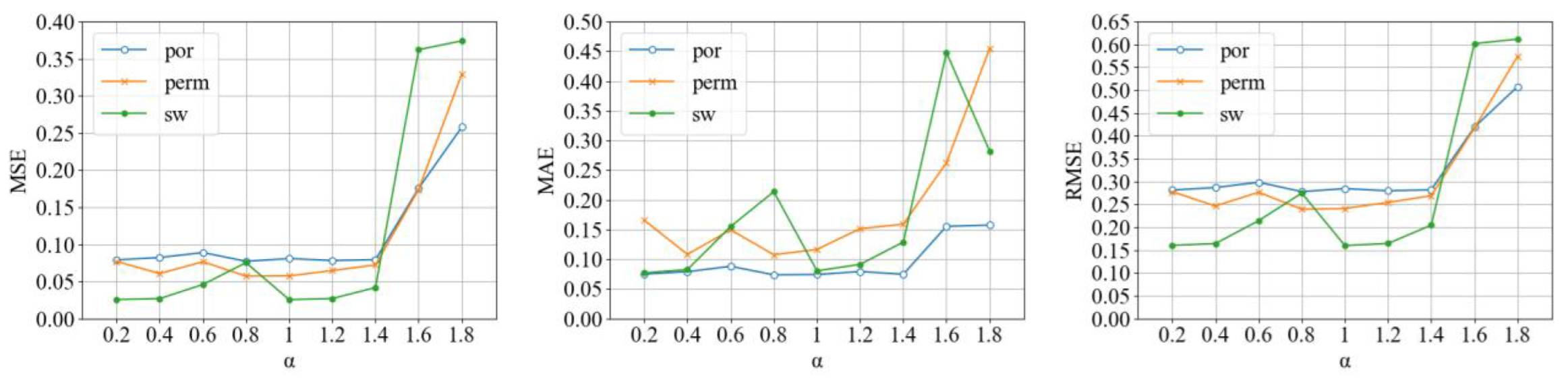
4.3. FTCN Parameter Setting

4.3.1. Setting α

We define α in Equation (2). The α is a balance factor of the fusional module in the FTCN model, and it is used to weigh the integration with the network layers. Its value represents the integration degree of the network layers. By adjusting α , we can better realize the integration of the network layers. In order to study the effect of various α for the experimental prediction results, the experimental values of α were 0.2, 0.4, 0.6, 0.8, 1, 1.2, 1.4, 1.6, 1.8 respectively.
As shown in Figure 9, the MSE, MAE and RMSE of the FTCN model in the prediction of three kinds of reservoir parameters can reach lower values when α = 1 . In the experiment of porosity prediction (shown as the blue line), changes in α have little influence on the prediction result except α = 1.8 and α = 1.6 . The FTCN model is relatively stable when α < = 1.4 . When α = 1.8 , the errors of porosity, permeability and water saturation become larger in varying degrees, indicating that α = 1.8 is not conducive to the prediction of the FTCN model. This shows that the larger the α value is, the less the effectiveness of the fusion of different network layers will be. When predicting water saturation, the difference between α = 0.2 and α = 1 is very small, and when α = 1 , the FTCN model performs best in permeability prediction. Considering three reservoir parameters, α = 1 is the optimal parameter for the FTCN model. In the follow-up experiments, α was set to 1.

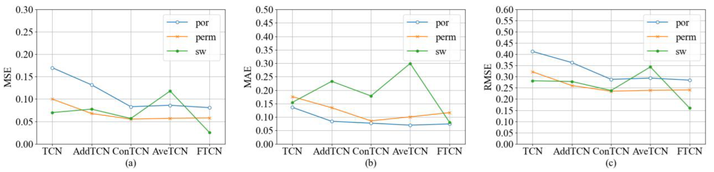
4.3.2. Verification of Fusional Module

For the sake of verifying the effect of the proposed fusional module, we compared it with the unimproved TCN and AddTCN, ConTCN and AveTCN combined with Add, Concat and Average fusion methods. Among them, Add, Concat and Average are all commonly used methods of network multi-layer feature fusion. In various network models, such as ResNet [44] and FPN [45], add is used to fuse features, while in DenseNet [46], concat is used to fuse features. Experiments were carried out in the prediction of three reservoir parameters that include porosity, permeability and water saturation. Among them,
(1)
AddTCN refers to the method of the add operation, which is to carry out a sum operation on the output of the merged layer to fuse the information;
(2)
ConTCN refers to the method of the concat operation, which splices the output of the layer to be merged along the last dimension and then fuses the information;
(3)
AveTCN refers to the method of the average operation, which fuses the output of the layer to be merged by the element mean.
As shown in Figure 10, the FTCN model is superior to the TCN model in predicting porosity (por), permeability (perm) and water saturation (sw) in MAE, MSE and RMSE. In the experiment of predicting porosity, the predictive result of the FTCN model is obviously better than AddTCN and is very similar to that of ConTCN and AveTCN. When predicting permeability, ConTCN has the best performance, and the evaluation metrics obtained by FTCN are slightly higher than ConTCN but also significantly lower than the TCN and AddTCN models. In the experiment of predicting water saturation, the performance of the FTCN model is superior to other models and achieves the best prediction effect. This may be because the fusional module is more suitable for the information fusion of different layers in the reservoir parameter prediction network compared with other fusional methods.

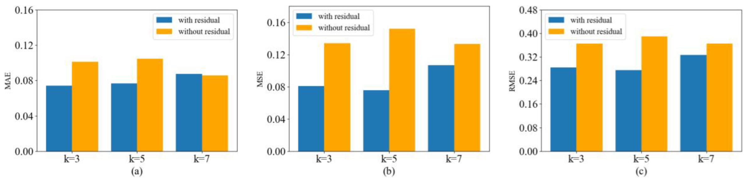
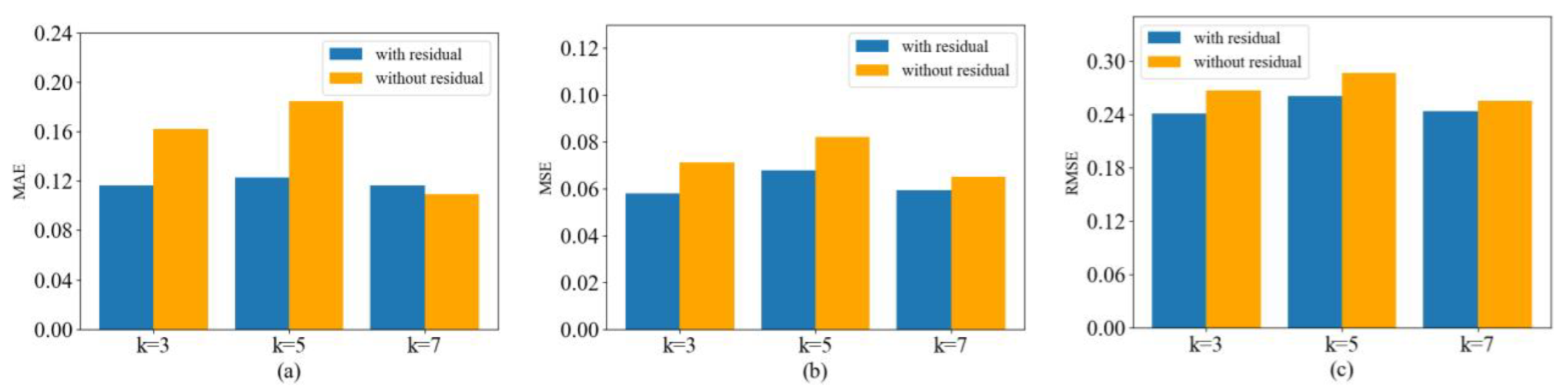
4.3.3. Influence of Filter Size k and Residual Block

We explore the influence of the filter size (k) and residual block in the FTCN model based on experiments. The effect of porosity predicted by the FTCN model is demonstrated in Figure 11.
The MAE reaches the lowest level when k = 3 and the residual block exists. The MSE of the model with the residual block is significantly better than that of the model without the residual block when k = 3 , k = 5 and k = 7 . When looking at the RMSE, the performance is relatively better when k = 5 , and the model with the residual block also has a better performance.
We also explore the performance of the FTCN model for predicting permeability. As illustrated in Figure 12, this model has the best effect when k = 3 , and the performance of this model with the residual block is better as a whole.
We also explored the experiment of the FTCN model for predicting water saturation. As shown in Figure 13, when k = 3 , the model performs better than k = 5 and k = 7 on MAE, MSE and RMSE, and the model with the residual block is better than the FTCN model without the residual block.
From the above experiments on the FTCN model predicting porosity, permeability and water saturation, it can be seen that the prediction effect of the model with k = 3 and the residual block is better. That is because it avoids the degradation of the very deep network and advances the effect of the network.

4.4. Influence of Input Logging Curves

For the purpose of estimating the validity of the optimized logging curves used for the reservoir parameter prediction, the effects of different input logging curves on the experimental prediction results are explored.
In logging interpretation, permeability is related to porosity, and the commonly used three-porosity logging includes acoustic travel time, density and compensated neutron logging curves. Acoustic logging mainly measures the time difference of formation sliding waves. Using the interaction between gamma ray and formation, density logging can reflect the formation porosity by measuring the gamma count of gamma rays emitted by the source and arriving at the detector after one or more scatterings through the formation. The compensated neutron logging mainly reflects the deceleration ability of the formation to fast neutrons and shows the change of hydrogen content in the formation. They have different responses in different formations, are closely related to the determination of porosity, and have great advantages in calculating porosity, permeability and fluid properties. In addition, natural gamma ray and spontaneous potential curves are also often used to assist calculation. Natural gamma logging measures natural radioactivity in strata. Spontaneous potential logging is used to measure the variation of the potential naturally generated on the shaft with depth in an open hole so as to study the stratigraphic properties of the well profile. In the permeability prediction experiment, we split all the input logs into three different input log sets. Among them,
(1)
Curve_Set1 contains the acoustic travel time, density, compensated neutron logging, natural gamma ray, and spontaneous potential, which are closely related to porosity.
(2)
Curve_Set2 adds micro potential resistivity, micro-gradient resistivity, deep and medium investigation induction log, and high-definition induction logging curve M2R10, which are closely related to permeability calculation to the Curve_Set1.
(3)
Curve_Set3 contains all the input logs used for permeability prediction in this paper.
As shown in Figure 14, compared with Curve_ Set1, the prediction error of the Curve_Set2 experiment is significantly lower in MSE and RMSE. The results of MAE, MSE and RMSE of Curve_Set3 are all optimal, but it performs significantly better than Curve_Set1 and slightly lower than Curve_Set2. The reason may be that Curve_Set3 is very similar to the Curve_Set2, except that Curve_Set3 has several additional high-definition induction logging curves of different feet, which are very similar to the M2R10 logging curve in Curve_Set2. In practical applications, it can be considered to reduce the cost of logging by removing the high-resolution array induction logs of different feet and retain only the M2R10.

4.5. Comparison of Methods

For the purpose of estimating the effectiveness of the FTCN prediction method proposed in this paper, a series of comparative experiments are carried out to compare the proposed FTCN with LSTM, GRU and unimproved TCN. In our experiments, we employed the adaptive learning rate RMSProp algorithm to optimize the network. The initial learning rate was set to 0.001, and batch size the batch size was set to 32 to predict reservoir parameters such as porosity (POR), permeability (PERM) and water saturation (SW).
We used 20 % of the logging data samples to test, and the results are shown in Table 1. The RMSE of the FTCN model in porosity prediction is 0.23, 0.19 and 0.13 lower than the LSTM, GRU and TCN models, respectively. For the purpose of estimating the effect of the FTCN prediction model on different reservoir parameters, the FTCN model is used to predict permeability and water saturation. The MAE, MSE and RMSE of the FTCN model reach 0.12, 0.06 and 0.24, respectively. The MAE, MSE and RMSE predicted by the FTCN model are 0.08, 0.03 and 0.16, respectively, and the RMSE is 0.25 and 0.2 lower than the LSTM and GRU model, respectively. The possible reason is that the FTCN model’s fusional module considers the effects of different network layers and learns more accurate response relationships comprehensively. It can make better use of logging curves; thus, it achieves better performance than other methods. Compared with LSTM, GRU and TCN models, the FTCN model has a more accurate prediction effect and stable performance in the prediction of different reservoir parameters.
Figure 15, Figure 16 and Figure 17 show the experimental results of reservoir parameters predicted by the four models, respectively. It can be seen that the LSTM and GRU models can predict the parameter values at different depths of the reservoir roughly, but there is a prediction deviation in the detailed value of the curves. The prediction performance of TCN is better than the former, but the problem is still not solved. The FTCN model more accurately reflects the slight fluctuations in the curve, and its prediction results are more consistent with real reservoir conditions. This may be because of the design of the unique fusional module in FTCN, which makes it achieve better results than other methods. In addition, as shown in Figure 15, the lower parts of the well section are water-flooded layers, and the upper part is a mudstone section, which reflects the characteristics of this area.

5. Conclusions and Future Works

Reservoir parameter prediction is exceedingly significant in petroleum exploration and development. Predicting reservoir parameters effectively can provide a reference for analyzing reservoir properties and assist interpreters in evaluating oil and gas reservoirs. In this paper, a reservoir parameter prediction method named FTCN is proposed. Firstly, a fusion module is designed to fully exploit the nonlinear mapping on curves by using data information of different network layers, which makes our method more sensitive to the relationship between logging curves and reservoir parameters. Secondly, we design the structure of the FTCN. Dilated causal convolution and residual connection are taken, which expands the receptive field of the network so that the effective information obtained is richer and the model is more stable. At last, experiments on real logging datasets show that the prediction results of FTCN are more consistent with the real formation conditions in reservoir parameter prediction, even if there are great changes in stratus. Therefore, our work can provide a reference for well interpreters to analyze reservoirs.
The reservoir parameter prediction effect may be improved by selecting representative and sensitive curves. In the future, we will conduct research in many different exploration areas, and further study the improved reservoir parameter prediction method by considering the curve quality improvement and the response curve selection strategy to improve the prediction effect under poor geological environments and imperfect well data. Additionally, we will explore whether considering the mixed application of multiple models for different strata can further enhance the anti-interference ability to improve the prediction effect.

Author Contributions

Conceptualization, H.Z. and K.F.; methodology, H.Z.; software, K.F.; validation, Z.L., Z.W. and J.S.; formal analysis, Z.L.; investigation, K.F.; resources, H.Z.; data curation, H.Y.; writing—original draft preparation, K.F.; writing—review and editing, H.Z., H.Y. and X.G.; visualization, Z.L.; supervision, Z.W.; project administration, J.S.; funding acquisition, H.Z. All authors have read and agreed to the published version of the manuscript.

Funding

This research was funded by The Major Scientific and Technological Projects of CNPC (No. ZD2019-183-004), The Fundamental Research Funds for the Central Universities (No. 20CX05019A) and Sponsored by CNPC Innovation Found (2021DQ02-0402).

Institutional Review Board Statement

Not applicable.

Informed Consent Statement

Not applicable.

Data Availability Statement

Not applicable.

Conflicts of Interest

The authors declare no conflict of interest.

References

  1. Xu, B.; Wu, H.; Feng, Z.; Li, Y.; Wang, K.; Liu, P. Application status and prospects of artificial intelligence in well logging and formation evaluation. Acta Pet. Sin. 2021, 42, 508–522. [Google Scholar]
  2. Rumelhart, D.E.; Hinton, G.E.; Williams, R.J. Learning representations by back-propagating errors. Nature 1986, 323, 533–536. [Google Scholar] [CrossRef]
  3. Hopfield, J.J. Neural networks and physical systems with emergent collective computational abilities. Proc. Natl. Acad. Sci. USA 1982, 79, 2554–2558. [Google Scholar] [CrossRef] [Green Version]
  4. Hochreiter, S.; Schmidhuber, J. Long short-term memory. Neural Comput. 1997, 9, 1735–1780. [Google Scholar] [CrossRef] [PubMed]
  5. Cho, K.; van Merrienboer, B.; Gulcehre, C.; Bougares, F.; Schwenk, H.; Bengio, Y. Learning phrase representations using RNN encoder-decoder for statistical machine translation. In Proceedings of the Conference on Empirical Methods in Natural Language Processing (EMNLP 2014), Doha, Qatar, 25–29 October 2014. [Google Scholar]
  6. dos Santos, D.T.; Roisenberg, M.; dos Santos Nascimento, M. Deep Recurrent Neural Networks Approach to Sedimentary Facies Classification Using Well Logs. IEEE Geosci. Remote Sens. Lett. 2021, 19, 1–5. [Google Scholar] [CrossRef]
  7. Al-Shabandar, R.; Jaddoa, A.; Liatsis, P.; Hussain, A.J. A deep gated recurrent neural network for petroleum production forecasting. Mach. Learn. Appl. 2021, 3, 100013. [Google Scholar] [CrossRef]
  8. Heghedus, C.; Shchipanov, A.; Rong, C. Advancing deep learning to improve upstream petroleum monitoring. IEEE Access 2019, 7, 106248–106259. [Google Scholar] [CrossRef]
  9. Kuanzhi, Z.; Zhang, L.; Zheng, D.; Chonghao, S.; Qingning, D. A reserve calculation method for fracture-cavity carbonate reservoirs in Tarim Basin, NW China. Pet. Explor. Dev. 2015, 42, 277–282. [Google Scholar]
  10. Al-Jawad, S.N.; Saleh, A.H.; Al-Dabaj, A.A.A.; Al-Rawi, Y.T. Reservoir flow unit identification of the Mishrif formation in North Rumaila Field. Arab. J. Geosci. 2014, 7, 2711–2728. [Google Scholar] [CrossRef]
  11. Yu, Y.; Wang, C.; Gu, X.; Li, J. A novel deep learning-based method for damage identification of smart building structures. Struct. Health Monit. 2019, 18, 143–163. [Google Scholar] [CrossRef] [Green Version]
  12. Yu, Y.; Rashidi, M.; Samali, B.; Mohammadi, M.; Nguyen, T.N.; Zhou, X. Crack detection of concrete structures using deep convolutional neural networks optimized by enhanced chicken swarm algorithm. Struct. Health Monit. 2022, 14759217211053546. [Google Scholar] [CrossRef]
  13. Sircar, A.; Yadav, K.; Rayavarapu, K.; Bist, N.; Oza, H. Application of machine learning and artificial intelligence in oil and gas industry. Pet. Res. 2021, 6, 379–391. [Google Scholar] [CrossRef]
  14. Choubey, S.; Karmakar, G. Artificial intelligence techniques and their application in oil and gas industry. Artif. Intell. Rev. 2021, 54, 3665–3683. [Google Scholar] [CrossRef]
  15. Janjuhah, H.T.; Kontakiotis, G.; Wahid, A.; Khan, D.M.; Zarkogiannis, S.D.; Antonarakou, A. Integrated Porosity Classification and Quantification Scheme for Enhanced Carbonate Reservoir Quality: Implications from the Miocene Malaysian Carbonates. J. Mar. Sci. Eng. 2021, 9, 1410. [Google Scholar] [CrossRef]
  16. Adeniran, A.A.; Adebayo, A.R.; Salami, H.O.; Yahaya, M.O.; Abdulraheem, A. A competitive ensemble model for permeability prediction in heterogeneous oil and gas reservoirs. Appl. Comput. Geosci. 2019, 1, 100004. [Google Scholar] [CrossRef]
  17. Liu, J.J.; Liu, J.C. An intelligent approach for reservoir quality evaluation in tight sandstone reservoir using gradient boosting decision tree algorithm-A case study of the Yanchang Formation, mid-eastern Ordos Basin, China. Mar. Pet. Geol. 2021, 126, 104939. [Google Scholar] [CrossRef]
  18. Yong Hong, W.; Zhengnan, Z.; Shufa, Z. Estimation of porosity using seismic and logging data. Oil Geophys. Prospect. 1990, 25, 572–577. [Google Scholar]
  19. Jinzhong, Z. An Empirical Formula for Estimating Permeability Based on Well Logging Data and Its Physuical Background Analysis. J. Xi’an Shiyou Univ. 1991, 6, 16–20. [Google Scholar]
  20. Xie, J.; Chen, W.; Zhang, D.; Zu, S. Application of principal component analysis in weighted stacking of seismic data. IEEE Geosci. Remote Sens. Lett. 2017, 14, 1213–1217. [Google Scholar] [CrossRef]
  21. Inyang, N.J.; Agbasi, O.E.; Akpabio, G.T. Integrated analysis of well logs for productivity prediction in sand-shale sequence reservoirs of the Niger Delta—A case study. Arab. J. Geosci. 2021, 14, 1–9. [Google Scholar] [CrossRef]
  22. Kuang, L.; He, L.; Yili, R.; Kai, L.; Mingyu, S.; Jian, S.; Xin, L. Application and development trend of artificial intelligence in petroleum exploration and development. Pet. Explor. Dev. 2021, 48, 1–14. [Google Scholar] [CrossRef]
  23. Otchere, D.A.; Ganat, T.O.A.; Gholami, R.; Ridha, S. Application of supervised machine learning paradigms in the prediction of petroleum reservoir properties: Comparative analysis of ANN and SVM models. J. Pet. Sci. Eng. 2021, 200, 108182. [Google Scholar] [CrossRef]
  24. Zhu, P.; Lin, C.; Wu, P.; Fan, R.; Zhang, H.; Pu, W. Permeability prediction of tight sandstone reservoirs using improved BP neural network. Open Pet. Eng. J. 2015, 8, 288–292. [Google Scholar] [CrossRef] [Green Version]
  25. Mahdaviara, M.; Rostami, A.; Keivanimehr, F.; Shahbazi, K. Accurate determination of permeability in carbonate reservoirs using Gaussian Process Regression. J. Pet. Sci. Eng. 2021, 196, 107807. [Google Scholar] [CrossRef]
  26. Gholami, R.; Shahraki, A.; Paghaleh, M.J. Prediction of Hydrocarbon Reservoirs Permeability Using Support Vector Machine. Math. Probl. Eng. 2012, 2012, 670723. [Google Scholar] [CrossRef] [Green Version]
  27. Li, K.; Zhou, G.; Yang, Y.; Li, F.; Jiao, Z. A novel prediction method for favorable reservoir of oil field based on grey wolf optimizer and twin support vector machine. J. Pet. Sci. Eng. 2020, 189, 106952. [Google Scholar] [CrossRef]
  28. Akande, K.O.; Owolabi, T.O.; Olatunji, S.O.; AbdulRaheem, A. A hybrid pARTICLE swarm optimization and support vector regression model for modelling permeability prediction of hydrocarbon reservoir. J. Pet. Sci. Eng. 2017, 150, 43–53. [Google Scholar] [CrossRef]
  29. Okon, A.N.; Adewole, S.E.; Uguma, E.M. Artificial neural network model for reservoir petrophysical properties: Porosity, permeability and water saturation prediction. Model. Earth Syst. Environ. 2021, 7, 2373–2390. [Google Scholar] [CrossRef]
  30. Hamidi, H.; Rafati, R. Prediction of oil reservoir porosity based on BP-ANN. In Proceedings of the 2012 International Conference on Innovation Management and Technology Research, Malacca, Malaysia, 21–22 May 2012; pp. 241–246. [Google Scholar]
  31. Xiang, Y.F.; Kang, Z.H.; Hao, W.J.; Fu, K.N.; Wang, F.S. A Composite Method of Reservoir Parameter Prediction Based on Linear Regression and Neural Network. Sci. Technol. Eng. 2017, 17, 46–52. [Google Scholar]
  32. Nasir, I.M.; Bibi, A.; Shah, J.H.; Khan, M.A.; Sharif, M.; Iqbal, K.; Nam, Y.; Kadry, S. Deep learning-based classification of fruit diseases: An application for precision agriculture. CMC-Comput. Mater. Contin. 2021, 66, 1949–1962. [Google Scholar] [CrossRef]
  33. Ouahabi, A.; Taleb-Ahmed, A. Deep learning for real-time semantic segmentation: Application in ultrasound imaging. Pattern Recognit. Lett. 2021, 144, 27–34. [Google Scholar] [CrossRef]
  34. Muhammad, A.N.; Aseere, A.M.; Chiroma, H.; Shah, H.; Gital, A.Y.; Hashem, I.A.T. Deep learning application in smart cities: Recent development, taxonomy, challenges and research prospects. Neural Comput. Appl. 2021, 33, 2973–3009. [Google Scholar] [CrossRef]
  35. Yuyang, L.; Xinhua, M.; Xiaowei, Z.; Wei, G.; Lixia, K.; Rongze, Y.; Yuping, S. Shale gas well flowback rate prediction for Weiyuan field based on a deep learning algorithm. J. Pet. Sci. Eng. 2021, 203, 108637. [Google Scholar] [CrossRef]
  36. Zhao, J.; Wang, F.; Cai, J. 3D tight sandstone digital rock reconstruction with deep learning. J. Pet. Sci. Eng. 2021, 207, 109020. [Google Scholar] [CrossRef]
  37. An, P.; Cao, D.P.; Zhao, B.Y.; Yang, X.L.; Zhang, M. Reservoir physical parameters prediction based on LSTM recurrent neural network. Prog. Geophys. 2019, 34, 1849–1858. [Google Scholar]
  38. Chen, W.; Yang, L.; Zha, B.; Zhang, M.; Chen, Y. Deep learning reservoir porosity prediction based on multilayer long short-term memory network. Geophysics 2020, 85, WA213–WA225. [Google Scholar] [CrossRef]
  39. Zhang, Z.; Wang, Y.; Wang, P.; Dimitri, R. On a Deep Learning Method of Estimating Reservoir Porosity. Math. Probl. Eng. 2021, 2021, 6641678. [Google Scholar] [CrossRef]
  40. Bai, S.; Kolter, J.Z.; Koltun, V. An Empirical Evaluation of Generic Convolutional and Recurrent Networks for Sequence Modeling. In Proceedings of the 6th International Conference on Learning Representations, Vancouver, BC, Canada, 30 April–3 May 2018. [Google Scholar]
  41. Gehring, J.; Auli, M.; Grangier, D.; Yarats, D.; Dauphin, Y.N. Convolutional sequence to sequence learning. In Proceedings of the International Conference on Machine Learning, Sydney, Australia, 6–11 August 2017; pp. 1243–1252. [Google Scholar]
  42. Tieleman, T.; Hinton, G. Divide the gradient by a running average of its recent magnitude. COURSERA Neural Netw. Mach. Learn. 2012, 6, 26–31. [Google Scholar]
  43. Yu, F.; Koltun, V. Multi-scale context aggregation by dilated convolutions. In Proceedings of the International Conference on Learning Representations, San Juan, Puerto Rico, 2–4 May 2016. [Google Scholar]
  44. He, K.; Zhang, X.; Ren, S.; Sun, J. Deep residual learning for image recognition. In Proceedings of the IEEE Conference on Computer Vision and Pattern Recognition, Las Vegas, NV, USA, 27–30 June 2016; pp. 770–778. [Google Scholar]
  45. Lin, T.Y.; Dollár, P.; Girshick, R.; He, K.; Hariharan, B.; Belongie, S. Feature pyramid networks for object detection. In Proceedings of the IEEE Conference on Computer Vision and Pattern Recognition, Honolulu, HI, USA, 21–26 July 2017; pp. 2117–2125. [Google Scholar]
  46. Huang, G.; Liu, Z.; Van Der Maaten, L.; Weinberger, K.Q. Densely connected convolutional networks. In Proceedings of the IEEE Conference on Computer Vision and Pattern Recognition, Honolulu, HI, USA, 21–26 July 2017; pp. 4700–4708. [Google Scholar]
Figure 1. Framework of reservoir parameter prediction model named FTCN.
Energies 15 05680 g001
Figure 2. Causal convolution.
Energies 15 05680 g002
Figure 3. Dilated convolution.
Energies 15 05680 g003
Figure 4. Situation in the study area. (a) the map of the location of the study area; (b) the relative position of the well and architecture analysis.
Energies 15 05680 g004
Figure 5. Different sedimentary facies in the study area.
Energies 15 05680 g005
Figure 6. The cross-plots of logging curve correlations. Shown are the AC-POR cross-plot, CNL-POR cross-plot, DEN-POR cross-plot, GR-POR cross-plot and SP-POR cross-plot, respectively. These show the correlation between different logging curves and POR.
Energies 15 05680 g006
Figure 7. The core images of well2. (a) trough cross-bedding gravelly sandstone facies; (b) massive bedding gravelly sandstone facies; (c) wavy cross bedding siltstone facies; (d) horizontal-bedding siltstone facies; (e) trough cross-bedding sandstone facies; (f) planar cross-bedding sandstone facies; (g) parallel-bedding sandstone facies; (h) massive mudstone facies.
Energies 15 05680 g007
Figure 8. Sedimentary structure characteristics of cored well5. (a) retained conglomerate facies; (b) trough cross-bedded sandstone facies; (c) tabular cross-bedded sandstone facies; (d) parallel-bedding sandstone facies; (e) wavy-bedding siltstone facies; (f) massive mudstone facies.
Energies 15 05680 g008
Figure 9. The influence of different α on FTCN model.
Energies 15 05680 g009
Figure 10. Influence of different fusion methods on the TCN model. (a) the MSE; (b) the MAE; (c) the RMSE.
Energies 15 05680 g010
Figure 11. Effect of different k and residual blocks on FTCN-predicted porosity. (a) the MAE; (b) the MSE; (c) the RMSE.
Energies 15 05680 g011
Figure 12. Effect of different k and residual blocks on FTCN predicted permeability. (a) the MAE; (b) the MSE; (c) the RMSE.
Energies 15 05680 g012
Figure 13. Influence of different k and residual blocks on FTCN-predicted water saturation. (a) the MAE; (b) the MSE; (c) the RMSE.
Energies 15 05680 g013
Figure 14. Comparison of different logging input sets.
Energies 15 05680 g014
Figure 15. Contrast of permeability prediction of distinct models.
Energies 15 05680 g015
Figure 16. Contrast of porosity prediction of distinct models.
Energies 15 05680 g016
Figure 17. Contrast of water saturation prediction of distinct models.
Energies 15 05680 g017
Table 1. Prediction performance of four models in three reservoir parameters.
PORPERMSW
MethodMAEMSERMSEMAEMSERMSEMAEMSERMSE
LSTM0.230.260.510.280.230.480.220.170.41
GRU0.170.220.470.250.190.440.200.130.36
TCN0.130.170.410.170.100.320.150.070.28
FTCN0.070.080.280.120.060.240.080.030.16
Publisher’s Note: MDPI stays neutral with regard to jurisdictional claims in published maps and institutional affiliations.

