Tracking and Rejection of Biased Sinusoidal Signals Using Generalized Predictive Controller

Abstract

Some novel applications require the tracking/rejection of biased sinusoidal reference/distur-bances. According to the internal model principle (IMP), a controller must embed the model of a biased sinusoidal signal to track references and also reject perturbations modeled through the aforementioned signal. However, the design of that kind of controller is not straightforward, especially when they are implemented in digital processors. This paper presents a controller, based on generalized predictive control (GPC), designed for tracking/rejection of biased sinusoidal signals. In general, GPC is based on the prediction of the plant responses through an augmented prediction model. The proposed approach develops an augmented model that predicts the future errors. The prediction model and the control law used in the proposed approach embed the discrete-time model of a biased sinusoidal signal. Thus, the proposed controller can track/reject biased sinusoidal references/disturbances. The predicted errors and the future inputs of the proposed augmented model are used to define the cost function that measures the control performance. An optimization technique was applied to obtain the solution of the cost function, which is the optimal sequence of future model inputs that allows defining the control law. Experimental tests prove that the proposed controller can asymptotically track and reject biased sinusoidal signals.

1. Introduction

Applications such as active vibration control, active rotor balancing, mechanics, magnetic bearings, and others require tracking/rejection of periodical signals [1,2,3,4]. In this context, tracking/rejection of biased sinusoidal signals (sine wave with a DC component) is applied in some novel applications [5]. Disturbances in some electro-hydraulic actuators can be modeled as biased sinusoidal signals [6]. The helicopter control system in [7] defines the vertical (bias) thrust while rejecting sinusoidal disturbance. Some novel permanent-magnet machines [8,9,10] and vernier machines [11,12] require biased sinusoidal stator currents to operate. The decoupling capacitor voltage of the inverter in [13] is a biased sine wave to compensate for the ripple power produced by the grid. The control of a Boost converter [14] is done to produce a unipolar voltage at the output converter. Those applications apply PI controllers, proportional-resonant controllers, Lyapunov functions, among other control techniques.

According to the internal model principle (IMP), a control system must embed the model of the reference/disturbance to be tracked/rejected [15,16]. However, inserting the signal model into a digital controller is non-trivial. For example, stable digital implementation of resonant controllers (used to track sine references) is difficult to achieve [17]. Thus, the design of a control system that tracks/rejects biased sinusoidal reference/disturbance is not straightforward. The resonant controller based on generalized predictive control (GPC) described in [18] was implemented in a DSP and strictly satisfied IMP. GPC uses an augmented model to predict future plant responses. GPC has a good transient response and constraints can be easily included [19,20,21]. However, the approach in [18] was not designed to track/reject biased-sinusoidal signals.

This paper present a novel GPC system whose augmented model embeds the poles of the $\mathcal{Z}$-transform of a biased sinusoidal signal. Thus, according to IMP, the proposed approach can asymptotically track/reject biased sinusoidal references/disturbance while having all the advantages of GPC. According to the author’s literature review, there is no other controller that embeds the model of a biased-sinusoidal signal and with experimental validation. Optimization technique allows the obtaining of the control law. Experimental tests using a DSP prove that the proposed approach can track/reject biased sinusoidal references/disturbances. The proposed approach was developed for a SISO (Single-Input Single-Output) plant. However, the proposed approach can be easily adapted for MIMO (Multiple-Input Multiple-Output) plants.

The paper is organized as follows. Firstly, the proposed approach is explained. After this, the experimental tests presented in this work prove that the proposed approach can track/reject sinusoidal biased references/disturbances. Conclusions are outlined. In this work, i represents the discrete-time, $I_n$ represents an $n\times n$ identity matrix, $0_{n\times m}$ denotes an $n\times m$ matrix composed by zeros, while $\mathcal{Z}\left\{\right\}$ denotes the $\mathcal{Z}$-transform. The signals are sampled with a period of $t_s$.

2. Proposed GPC Approach

2.1. Preliminaries

Equation (1) represents the model of a continuous-time biased sinusoidal reference:

$$r\left(t\right)=b+\rho sin\left(\omega t\right),$$

(1)

where t is time, $\omega$ is the frequency, $\rho$ is the amplitude and b is the bias. Let us consider that the state signals and reference are sampled with a sampling period equal to $t_s$. Thus, the discrete-time reference $r\left(i\right)$ is obtained by making $t=t_{s}i$, as follows:

$$r\left(i\right)=b+\rho sin(\Omega i),\Omega =\omega t_s.$$

(2)

The trigonometrical identities $sin\left(\alpha \right)-sin\left(\beta \right)=2sin\left(\frac{\alpha -\beta }{2}\right)cos\left(\frac{\alpha +\beta }{2}\right)$ and $sin\left(3\psi \right)=(2cos(2\psi )+1)sin\left(\psi \right)$ allow proving (3) and (4):

$$\begin{array}{cc}\hfill r\left(i\right)-r(i-1)& =b+\rho sin(\Omega i)-[b+\rho sin(\Omega (i-1)\left)\right]\hfill \\ \hfill & =\rho \left[sin(\Omega i)-sin\left(\Omega (i-1)\right)\right]\hfill \\ \hfill & =2\rho sin(0.5\Omega )cos(\Omega i-0.5\Omega ),\hfill \end{array}$$

(3)

$$\begin{array}{cc}\hfill r(i+1)-r(i-2)& =b+\rho sin(\Omega (i+1\left)\right)-[b+\rho sin(\Omega (i-2)\left)\right]\hfill \\ \hfill & =\rho \left[sin\left(\Omega (i+1)\right)-sin\left(\Omega (i-2)\right)\right]\hfill \\ \hfill & =2\rho sin\left(3(0.5\Omega )\right)cos(\Omega i-0.5\Omega )\hfill \\ \hfill & =2\left(2cos(\Omega )+1\right)\left[\rho sin(0.5\Omega )cos(\Omega i-0.5\Omega )\right].\hfill \end{array}$$

(4)

Replacing (3) into (4) allows proving (5):

$$r(i+1)=\gamma r\left(i\right)-\gamma r(i-1)+r(i-2),\gamma =2cos(\Omega )+1.$$

(5)

2.2. Proposed Augmented Model

Equations (6) and (7) describe the n-order discrete-time space-state model of a SISO (Single-Input Single-Output) plant, while (8) defines the discrete-time tracking error $e\left(i\right)$:

$$\begin{array}{c}x(i+1)=Ax\left(i\right)+Bu\left(i\right),\end{array}$$

(6)

$$\begin{array}{c}y\left(i\right)=Cx\left(i\right),\end{array}$$

(7)

$$\begin{array}{c}e\left(i\right)=r\left(i\right)-y\left(i\right)=r\left(i\right)-Cx\left(i\right),\end{array}$$

(8)

where $x\left(i\right)\in {\Re }^{n\times 1}$ is the state vector, $u\left(i\right)$ is the input, $y\left(i\right)$ is the output, $A\in {\Re }^{n\times n},B\in {\Re }^{n\times 1}$ and $C\in {\Re }^{1\times n}$. The discrete-time model in (6) and (7) is obtained applying a discretization process into the continuous-time plant model [22]. The plant transfer function, $G\left(z\right)$, can be defined in terms of A, B and C:

$$G\left(z\right)=C{\left(z{I}_n-A\right)}^{-1}B.$$

(9)

According to (8), the future error is $e(i+1)=r(i+1)-Cx(i+1)$. Using (5), $e(i+1)$ can be expressed as in (10):

$$e(i+1)=\underset{r(i+1)}{\underbrace{\gamma r\left(i\right)-\gamma r(i-1)+r(i-2)}}-Cx(i+1).$$

(10)

Equation (8) allows us to deduce that $r(i-k)=e(i-k)+Cx(i-k),k=0,1,2,3$. Thus, (10) can be rewritten as follows:

$$\begin{array}{cc}\hfill e(i+1)& =\gamma \underset{r\left(i\right)}{\underbrace{\left[e\right(i)+Cx(i\left)\right]}}-\gamma \underset{r(i-1)}{\underbrace{\left[e\right(i-1)+Cx(i-1\left)\right]}}+\underset{r(i-2)}{\underbrace{\left[e\right(i-2)+Cx(i-2\left)\right]}}-Cx(i+1)\hfill \\ \hfill & =\gamma e\left(i\right)-\gamma e(i-1)+e(i-2)+C\left[x\right(i-2)-\gamma x(i-1)+\gamma x(i)-x(i+1\left)\right].\hfill \end{array}$$

(11)

Let define $q\left(i\right)$ and $v\left(i\right)$ as follows:

$$\begin{array}{c}q\left(i\right)=x(i-3)-\gamma x(i-2)+\gamma x(i-1)-x\left(i\right),\end{array}$$

(12)

$$\begin{array}{c}v\left(i\right)=u(i-3)-\gamma u(i-2)+\gamma u(i-1)-u\left(i\right).\end{array}$$

(13)

Equations (6) and (12) allow the deduction of (14) and (15):

$$\begin{array}{c}x(i+1-k)=Ax(i-k)+Bu(i-k),k=0,1,2,3,\end{array}$$

(14)

$$\begin{array}{c}x(i-2)-\gamma x(i-1)+\gamma x\left(i\right)-x(i+1)=q(i+1).\end{array}$$

(15)

Applying (14) into (15), and according to the definitions of $q\left(i\right)$ and $v\left(i\right)$ in (12) and (13), $q(i+1)$ can be expressed as in (16):

$$\begin{array}{cc}\hfill q(i+1)& =\left[Ax(i-3)+Bu(i-3)\right]-\gamma \left[Ax(i-2)+Bu(i-2)\right]\hfill \\ \hfill & +\gamma \left[Ax(i-1)+Bu(i-1)\right]-\left[Ax\left(i\right)+Bu\left(i\right)\right]\hfill \\ \hfill & =A\left[x(i-3)-\gamma x(i-2)+\gamma x(i-1)-x\left(i\right)\right]\hfill \\ \hfill & +B\left[u(i-3)-\gamma u(i-2)+\gamma u(i-1)-u\left(i\right)\right]\hfill \\ \hfill & =Aq\left(i\right)+Bv\left(i\right).\hfill \end{array}$$

(16)

Replacing (15) and (16) into (11), yields:

$$\begin{array}{cc}\hfill e(i+1)& =\gamma e\left(i\right)-\gamma e(i-1)+e(i-2)+q(i+1)\hfill \\ \hfill & =\gamma e\left(i\right)-\gamma e(i-1)+e(i-2)+CAq\left(i\right)+CBv\left(i\right).\hfill \end{array}$$

(17)

The matrix equation in (18) is deduced from (17):

$$\underset{\epsilon (i+1)}{\underbrace{\left[\begin{array}{c}e(i-1)\\ e\left(i\right)\\ e(i+1)\end{array}\right]}}=\underset{E}{\underbrace{\left[\begin{array}{ccc}0& 1& 0\\ 0& 0& 1\\ 1& -\gamma & \gamma \end{array}\right]}}\underset{\epsilon \left(i\right)}{\underbrace{\left[\begin{array}{c}e(i-2)\\ e(i-1)\\ e\left(i\right)\end{array}\right]}}+\underset{\sigma }{\underbrace{\left[\begin{array}{c}0\\ 0\\ 1\end{array}\right]}}CAq\left(i\right)+CBv\left(i\right).$$

(18)

On the other hand, note that:

$$\left[\begin{array}{cc}{0}_{1\times n}& {\sigma }^T\end{array}\right]\left[\begin{array}{c}q\left(i\right)\\ \epsilon \left(i\right)\end{array}\right]=\left[\begin{array}{ccc}0& 0& 1\end{array}\right]\left[\begin{array}{c}e(i-2)\\ e(i-1)\\ e\left(i\right)\end{array}\right]=e\left(i\right).$$

(19)

The proposed augmented model in (20) is defined using (16), (18) and (19):

$$\begin{array}{cc}\hfill \underset{\underline{x}(i+1)}{\underbrace{\left[\begin{array}{c}q(i+1)\\ \epsilon (i+1)\end{array}\right]}}& =\underset{\underline{\mathcal{A}}}{\underbrace{\left[\begin{array}{cc}A& 0_{n\times 3}\\ \sigma CA& E\end{array}\right]}}\underset{\underline{x}\left(i\right)}{\underbrace{\left[\begin{array}{c}q\left(i\right)\\ \epsilon \left(i\right)\end{array}\right]}}+\underset{\underline{\mathcal{B}}}{\underbrace{\left[\begin{array}{c}B\\ \sigma CB\end{array}\right]}}v\left(i\right)\hfill \\ \hfill \mathrm{Output}:e\left(i\right)& =\underset{\underline{\mathcal{C}}}{\underbrace{\left[\begin{array}{cc}{0}_{1\times n}& {\sigma }^T\end{array}\right]}}\underline{x}\left(i\right),\hfill \end{array}$$

(20)

where $v\left(i\right)$ is the model input, $e\left(i\right)$ is the model output, $\underline{x}\left(i\right)$ is the model state vector, while $\underline{\mathcal{A}}\in {\Re }^{(n+3)\times (n+3)}$, $\underline{\mathcal{B}}\in {\Re }^{(n+3)\times 1}$ and $\underline{\mathcal{C}}\in {\Re }^{1\times (n+3)}$. It is assumed that the frequency $\omega$ is known to calculate $\gamma$. If not, estimators can be used to obtain $\omega$ [23,24]. The development of the augmented model in (20) is the main original contribution of this work in the design of predictive controller. The mathematical analysis presented in Section 3 will prove that this augmented model embeds the Z-transform of a biased-sinusoidal signal.

2.3. Predictive Control Law through GPC

GPC theory allows predicting the future outputs of the model in (20), i.e., the tracking errors. Let Y and U be the vectors composed of the future errors and the future prediction model inputs, respectively:

$$\begin{array}{c}Y={\left[e(i+1)e(i+2)\dots e(i+p)\right]}^T\in {\Re }^{p\times 1},\end{array}$$

(21)

$$\begin{array}{c}U={\left[v\left(i\right)v(i+1)\dots v(i+c-1)\right]}^T\in {\Re }^{c\times 1},\end{array}$$

(22)

where c and p are the size of the control horizon and the prediction horizon, respectively, such as $c\le p$. The value of Y can be obtained as follows [18]:

$$\begin{array}{c}Y=F\underline{x}\left(i\right)+\Phi U,\end{array}$$

(23)

$$\begin{array}{c}F=\left[\begin{array}{c}\underline{C}\underline{A}\\ \underline{C}{\underline{A}}^2\\ ⋮\\ \underline{C}{\underline{A}}^p\end{array}\right],\Phi =\left[\begin{array}{ccccc}\underline{C}\underline{B}& 0& 0& \dots & 0\\ \underline{C}\underline{A}\underline{B}& \underline{C}\underline{B}& 0& \dots & 0\\ \underline{C}{\underline{A}}^2\underline{B}& \underline{C}\underline{A}\underline{B}& \underline{C}\underline{B}& \dots & 0\\ ⋮& ⋮& ⋮& \ddots & ⋮\\ \underline{C}{\underline{A}}^{p-1}\underline{B}& \underline{C}{\underline{A}}^{p-2}\underline{B}& \dots & \dots & \underline{C}{\underline{A}}^{p-c}\underline{B}\end{array}\right],\end{array}$$

(24)

where $\underline{A}$, $\underline{B}$ and $\underline{C}$ are defined in (20). The cost function in (25) is commonly applied in GPC to obtain the optimal U through an optimization procedure [18,19,20]:

$$J=U^T{R}_{u}U+Y^{T}Y,R_u=r_u{I}_c,$$

(25)

where $r_u$ is a tuning parameter of the cost function: the larger the value of $r_u$, the reduction of the magnitude of U becomes more important in the optimization process [19]. The optimal solution of J makes $\frac{\partial J}{\partial U}=0$ [19]. Replacing (21) into (25) allows defining $\frac{\partial J}{\partial U}$ as in (26):

$$\frac{\partial J}{\partial U}=\frac{2{\varphi }^{T}F\underline{x}\left(i\right)+\left({\varphi }^T\varphi +R_u\right)U}{\partial U}=0.$$

(26)

Equation (27) defines the solution of (26) [18]. The receding horizon technique states that only the first element of U is used to estimate the control law. According to (22), that element is $v\left(i\right)=\left[10_{1\times (n-1)}\right]U$, which can be calculated through (28):

$$\begin{array}{c}U=-{\left({\Phi }^T\Phi +R_u\right)}^{-1}{\Phi }^{T}F\underline{x}\left(i\right).\end{array}$$

(27)

$$\begin{array}{c}v\left(i\right)=\underset{K_{bs}}{\underbrace{\left[10_{1\times (n-1)}\right]{\left({\Phi }^T\Phi +R_u\right)}^{-1}{\Phi }^{T}F}}\underline{x}\left(i\right).\end{array}$$

(28)

Substituting (28) into (13) allows deducing the plant input $u\left(i\right)$:

$$u\left(i\right)=u(i-3)+\gamma \left[u\right(i-1)-u(i-2\left)\right]-v\left(i\right).$$

(29)

Figure 1 shows the scheme of the proposed predictive controller.

3. Tracking/Rejecting Capability of the Proposed Controller

The sub-matrix algebra used in [18] allows the estimation of the transfer function of the model in (20), $G_a\left(z\right)$:

$$\begin{array}{cc}\hfill G_a\left(z\right)& =\underset{\underline{\mathcal{C}}}{\underbrace{\left[0_{1\times n}{\sigma }^T\right]}}\underset{z{I}_{n+3}-\underline{\mathcal{A}}}{\underbrace{{\left[\begin{array}{cc}Z{I}_n-A& 0_{n\times 3}\\ -\sigma CA& z{I}_3-E\end{array}\right]}^{-1}}}\underset{\underline{B}}{\underbrace{\left[\begin{array}{c}B\\ \sigma CB\end{array}\right]}}\hfill \\ \hfill & =\left[0_{1\times n}{\sigma }^T\right]\left[\begin{array}{cc}{\left(z{I}_n-A\right)}^{-1}& O\\ {\left(z{I}_3-E\right)}^{-1}\sigma CA{\left(z{I}_n-A\right)}^{-1}& {\left(z{I}_3-E\right)}^{-1}\end{array}\right]\left[\begin{array}{c}{I}_n\\ \sigma C{I}_{n}B\end{array}\right]\hfill \\ \hfill & ={\sigma }^T{\left(z{I}_3-E\right)}^{-1}\sigma C\left[A{\left(z{I}_n-A\right)}^{-1}+I_n\right]B\hfill \\ \hfill & ={\sigma }^T{\left(z{I}_3-E\right)}^{-1}\sigma C\left[A{\left(z{I}_n-A\right)}^{-1}+\left(z{I}_n-A\right){\left(z{I}_n-A\right)}^{-1}\right]B\hfill \\ \hfill & =z\left({\sigma }^T{\left(z{I}_3-E\right)}^{-1}\sigma \right)\left(C{\left(z{I}_n-A\right)}^{-1}B\right)\hfill \end{array}$$

(30)

Note that $z{I}_3-E=\left[\begin{array}{ccc}z& -1& 0\\ 0& z& -1\\ -1& \gamma & z-\gamma \end{array}\right]$. Let ${\left(z{I}_3-E\right)}^{-1}=\left[\begin{array}{ccc}{l}_{11}& l_{12}& l_{13}\\ l_{21}& l_{22}& l_{23}\\ l_{31}& l_{32}& l_{33}\end{array}\right]$. The adjoint method allows us to prove that $l_{33}={\displaystyle \frac{z^2}{det(z{I}_3-E)}}={\displaystyle \frac{z^2}{z^2(z-\gamma )+z\gamma -1}}$. Therefore:

$${\sigma }^T{\left(z{I}_3-E\right)}^{-1}\sigma =\left[\begin{array}{ccc}0& 0& 1\end{array}\right]\left[\begin{array}{ccc}{l}_{11}& l_{12}& l_{13}\\ l_{21}& l_{22}& l_{23}\\ l_{31}& l_{32}& l_{33}\end{array}\right]\left[\begin{array}{c}0\\ 0\\ 1\end{array}\right]=l_{33}={\displaystyle \frac{z^2}{z^2(z-\gamma )+z\gamma -1}}$$

(31)

Using (9) and (31) into (30) yields:

$$\begin{array}{cc}\hfill G_a\left(z\right)& =z\frac{z^2}{z^2\left[z-(2cos(\Omega )+1)\right]+z(2cos(\Omega )+1)-1}G\left(z\right)\hfill \\ \hfill & =\frac{z^3}{(z-1)\left(z^2-2cos(\Omega )z+1\right)}G\left(z\right).\hfill \end{array}$$

(32)

On the other hand, taking the $\mathcal{Z}$-transform of both sides of (13) allows us to obtain the transfer function between the plant input $u\left(i\right)$ and the GPC control action $v\left(i\right)$:

$$\frac{\mathcal{Z}\left\{u\right(i\left)\right\}}{\mathcal{Z}\left\{v\right(i\left)\right\}}=\frac{z^3}{1-\gamma z+\gamma z^2-z^3}=\frac{-z^3}{(z-1)\left(z^2-2cos(\Omega )z+1\right)}.$$

(33)

Let consider that $(z-1)\left(z^2-2cos(\Omega )z+1\right)$ and the numerator of $G\left(z\right)$ have no common roots. The $\mathcal{Z}$-transform of the unitary step and the sine signal $sin(\Omega i)$ are $\frac{z}{z-1}$ and $\frac{sin(\Omega )z}{z^2-2cos(\Omega )z+1}$, respectively. According to (32) and (33), the prediction model and the control law embed the poles that model the sine and step signals. Hence, the proposed predictive controller is capable to track/reject both sine and step signals, according to IMP. Thus, the controller is suitable for dealing with biased sinusoidal references/disturbances. The cost function in (25) and its solution in (27) are described in [18]. However, the development of the prediction model and the control law that embed the Z-transform of the biased-sinusoidal signal (to satisfy IMP) are the main contributions presented in this work.

Application of the Proposed Approach for MIMO Plants

Let $n_{in}$ and $n_{out}$ be the number of inputs and outputs of a MIMO (Multiple-Input Multiple-Output) plant. In that case $B\in {\Re }^{n\times n_{in}}$, $C\in {\Re }^{n_{out}\times n}$, $r\left(i\right)\in {\Re }^{n_{in}\times 1}$ and $y\left(i\right)\in {\Re }^{n_{out}\times 1}$ in (6) and (7). Note that $e\left(i\right)\in {\Re }^{n_{out}\times 1}$ and $v\left(i\right)\in {\Re }^{n_{in}\times 1}$. Equations (12), (13) and (16) can be still applied to obtain $q\left(i\right)$, $v\left(i\right)$ and $q(i+1)$ when $x\left(i\right)$ and $u\left(i\right)$ belong to a MIMO system. Only the structure of (18) will change.

Let assume that all the references that compose $r\left(i\right)$ have the same frequency $\Omega$. Hence, the term $\gamma =2cos(\Omega )+1$ will be the same for each reference. Under that consideration, it is easy to prove that (5), (10), (11) and (17) are still valid for a MIMO system. Thus, (18) can be rewritten as follows:

$$\underset{\epsilon (i+1)}{\underbrace{\left[\begin{array}{c}e(i-1)\\ e\left(i\right)\\ e(i+1)\end{array}\right]}}=\underset{E}{\underbrace{\left[\begin{array}{ccc}O& I_o& O\\ O& O& I_0\\ I_0& -\gamma I_0& \gamma I_0\end{array}\right]}}\underset{\epsilon \left(i\right)}{\underbrace{\left[\begin{array}{c}e(i-2)\\ e(i-1)\\ e\left(i\right)\end{array}\right]}}+\underset{\sigma }{\underbrace{\left[\begin{array}{c}O\\ O\\ I_0\end{array}\right]}}CAq\left(i\right)+CBv\left(i\right),$$

(34)

where O is an $n_{out}\times n_{out}$ matrix of zeros, while $I_0$ is an $n_{out}\times n_{out}$ identity matrix. The augmented model for a MIMO plant is obtained by replacing into (20) the terms $\epsilon$, E and $\sigma$ defined in (34). The procedure described in [25] can be used to obtain the GPC control law from the augmented model of a MIMO system. Further analysis should be done in the case that the references have different frequencies.

4. Results

Experimental tests were done to prove the good performance of the proposed controller. The plant with transfer function $G\left(s\right)=\frac{1.418\times {10}^{6}s+3.637\times {10}^8}{s^3+2179s^2+2.273\times {10}^{6}s+7.274\times {10}^8}$ was used during those tests. This plant was discretized considering $t_s$ = 0.5 ms. Thus, the matrices of the discrete-time model of the plant are $A=\left[\begin{array}{ccc}0.413& 0.454& 0\\ -0.240& 0.788& 0\\ -0.437& 0.422& 0.774\end{array}\right]$, $B=\left[\begin{array}{c}0.1331\\ 0.4528\\ 0.1273\end{array}\right]$ and $C=\left[001\right]$. Figure 2 shows the experimental setup. The DSP DSPACE DS1104 was used to implement and test the proposed approach. Two tests were performed to prove the effectiveness of the proposed controller:

• Test 1: tracking of biased sinusoidal references with zero perturbation.
• Test 2: rejection of biased sinusoidal perturbation with a constant reference.

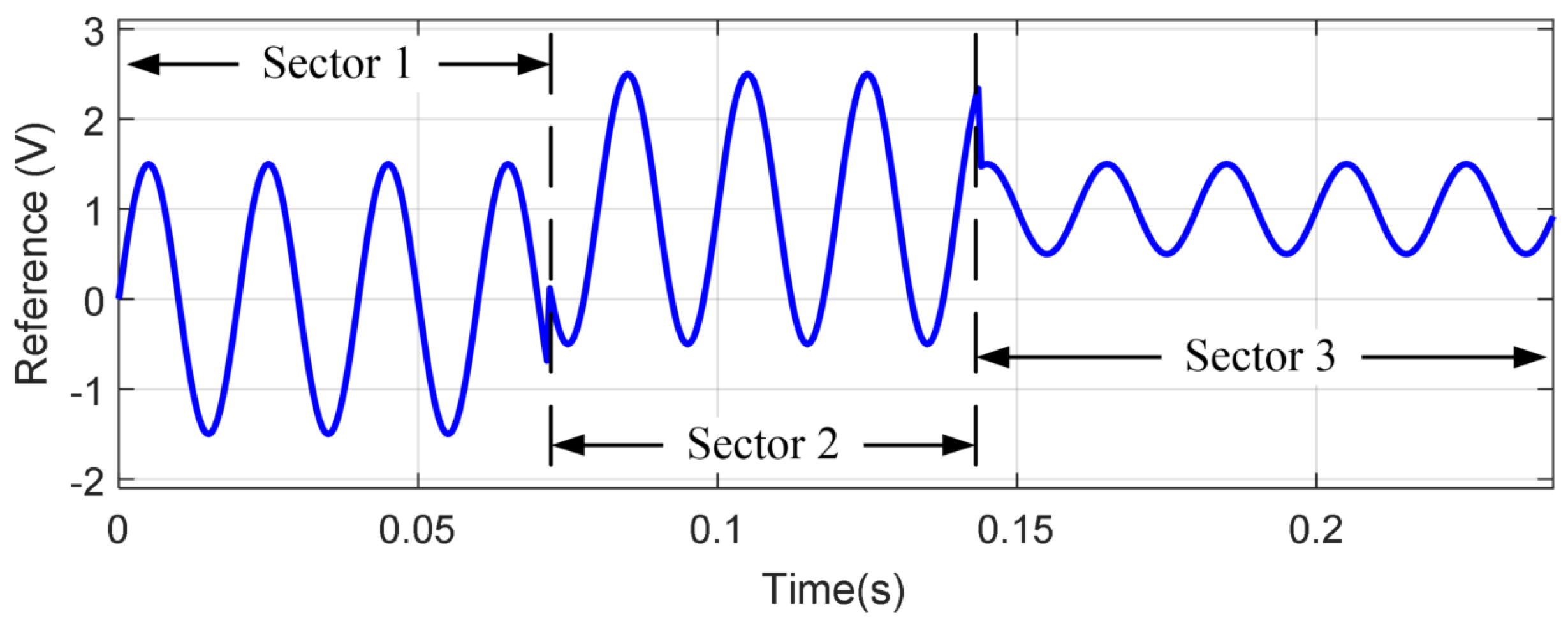
4.1. Test 1: Tracking of Biased Sinusoidal References

Figure 3 shows the reference used in test 1. This reference is composed by three sections which have different characteristics:

• Sector 1: bias (b) = 0 V, amplitude ($\rho$) = 1.5 V, $\omega =100\pi \frac{rad}{s}$ (50 Hz).
• Sector 2: bias (b) = 1 V, amplitude ($\rho$) = 1.5 V, $\omega =100\pi \frac{rad}{s}$ (50 Hz).
• Sector 3: bias (b) = 1 V, amplitude ($\rho$) = 0.5 V, $\omega =100\pi \frac{rad}{s}$ (50 Hz).

Table 1. RMSE for Test 1.

Configuration	RMSE	RMSE	RMSE	RMSE
($\mathit{p},\mathit{c},{\mathit{r}}_{\mathit{u}}$)	(Overall)	(Sector 1)	(Sector 2)	(Sector 3)
$20,1,0.3$	$130.8\times {10}^{-3}$	$152.1\times {10}^{-3}$	$123.3\times {10}^{-3}$	$118.6\times {10}^{-3}$
$20,1,0.07$	$130.9\times {10}^{-3}$	$152.3\times {10}^{-3}$	$122.9\times {10}^{-3}$	$118.7\times {10}^{-3}$
$40,20,0.07$	$147.9\times {10}^{-3}$	$166.9\times {10}^{-3}$	$153.9\times {10}^{-3}$	$126.6\times {10}^{-3}$

and

Table 2. Settling Time for Test 1.

Configuration	Settling Time	Settling Time	Settling Time
($\mathit{p},\mathit{c},{\mathit{r}}_{\mathit{u}}$)	(Sector 1)	(Sector 2)	(Sector 3)
$20,1,0.3$	$49.2\times {10}^{-3}$	$106.4\times {10}^{-3}$	$177.2\times {10}^{-3}$
$20,1,0.07$	$49.2\times {10}^{-3}$	$107.8\times {10}^{-3}$	$176.4\times {10}^{-3}$
$40,20,0.07$	$7.3\times {10}^{-3}$	$80.8\times {10}^{-3}$	$151.4\times {10}^{-3}$

show the root mean square error (RMSE) and the settling time (ST) of the proposed approach for different values of p, c, and $r_u$. The error and the control law obtained in this test are shown in Figure 4, Figure 5 and Figure 6. In all cases, the steady-state tracking error tends to zero and the settling time is small. The transient response depends on the setting of p, c and $r_u$.

4.2. Test 2: Rejection of Biased Sinusoidal Disturbance

Figure 7 shows the disturbance used in test 2, which is a biased sinusoidal signal from 0 to 0.12 s. The sinusoidal frequency of the perturbation is $\omega =100\pi \frac{rad}{s}$. The reference has a constant value of 1 V.

Table 3. RMSE for Test 2.

Configuration	RMSE	RMSE	RMSE
($\mathit{p},\mathit{c},{\mathit{r}}_{\mathit{u}}$)	(Overall)	(Sector 1)	(Sector 2)
$20,1,0.3$	$78.2\times {10}^{-3}$	$78.0\times {10}^{-3}$	$78.4\times {10}^{-3}$
$20,1,0.07$	$78.1\times {10}^{-3}$	$78.0\times {10}^{-3}$	$78.3\times {10}^{-3}$
$40,20,0.07$	$54.8\times {10}^{-3}$	$55.5\times {10}^{-3}$	$54.2\times {10}^{-3}$

and

Table 4. Settling Time for Test 2.

Configuration	Settling Time	Settling Time
($\mathit{p},\mathit{c},{\mathit{r}}_{\mathit{u}}$)	(Sector 1)	(Sector 2)
$20,1,0.3$	$74.7\times {10}^{-3}$	$168.0\times {10}^{-3}$
$20,1,0.07$	$101.6\times {10}^{-3}$	$168.5\times {10}^{-3}$
$40,20,0.07$	$62.2\times {10}^{-3}$	$126.9\times {10}^{-3}$

show the values of RMSE and the settling time after applying the disturbance. Figure 8, Figure 9 and Figure 10 show the error and the control law, for different values of p, c and $r_u$. The steady-state error tends to zero in all cases, proving that the biased sinusoidal disturbance was rejected.

5. Conclusions

This paper presents a new type of generalized predictive controller for the tracking/rejection of biased sinusoidal references/disturbances. The proposed controller satisfies the internal model principle (IMP), which is required to asymptotically track references and reject perturbations. Moreover, the proposed controller was defined in discrete time, avoiding the problems caused by the discretization process. IMP is a well-known technique for the design of control systems. However, as in the case of resonant controllers, the digital implementation of controllers that strictly satisfy IMP may be difficult to achieve. On the other hand, the proposed approach satisfies IMP and was experimentally validated. Equation (33) proves that the proposed controller embeds the model of the biased sinusoidal signal. However, Figure 1 shows that there is also a feedback of the plant states through $q\left(i\right)$. The development of the proposed prediction model was done to guarantee that the reference/perturbation model is embedded in the control law. The matrices of the proposed prediction model depend on the term $\sigma$ (which depends on the sinusoidal frequency). The proposed approach considers that the sinusoidal frequency is known. Further research should be done to adapt the proposed approach for variable sinusoidal frequencies (for example, adding frequency estimators). The transient response of the proposed controller depends on the selection of the GPC parameters p, c and $r_u$. There was no direct relationship between these parameters and the poles of the closed-loop system, but a heuristic method (e.g., differential evolution or genetic algorithm) can be applied to obtain the adequate GPC parameters. The proposed approach was elaborated for SISO plants. However, it can be adapted for MIMO plants when the references have the same frequency. Further research should be done to apply the controller for MIMO plants when the references have different frequencies. Resonant controllers (used to track sinusoidal references) have many applications in power electronics. For this reason, as future work, the proposed approach will be tested in a power electronics converter to track sinusoidal references while rejecting biased sinusoidal disturbances.

References

1. Kamaldar, M.; Hoagg, J.B. Adaptive Harmonic Control for Rejection of Sinusoidal Disturbances Acting on an Unknown System. IEEE Trans. Control Syst. Technol. 2020, 28, 277–290. [Google Scholar] [CrossRef]
2. Zhou, S.; Shi, J. Active Balancing and Vibration Control of Rotating Machinery: A Survey. Shock Vibrat. Dig. 2001, 33, 361–371. [Google Scholar] [CrossRef] [Green Version]
3. Esbrook, A.; Tan, X.; Khalil, H.K. An Indirect Adaptive Servocompensator for Signals of Unknown Frequencies with Application to Nanopositioning. Automatica 2013, 49, 2006–2016. [Google Scholar] [CrossRef]
4. Hong, F.; Du, C.; Tee, K.P.; Ge, S.S. Adaptive Disturbance Rejection in the Presence of Uncertain Resonance Mode in Hard Disk Drives. IEEE Trans. Inst. Meas. Control. 2010, 32, 99–119. [Google Scholar] [CrossRef] [Green Version]
5. Kim, W.; Moon, J. Adaptive Nonlinear Output Tracking Control With Rejection of Unmatched Biased Sinusoidal Disturbances for Nonlinear Systems. IEEE Access 2020, 8, 216210–216218. [Google Scholar] [CrossRef]
6. Kim, W.; Shin, D.; Won, D.; Chung, C.C. Disturbance-Observer-Based Position Tracking Controller in the Presence of Biased Sinusoidal Disturbance for Electrohydraulic Actuators. IEEE Trans. Control Syst. Technol. 2013, 21, 2290–2298. [Google Scholar] [CrossRef]
7. Ji, W.; Tian, B.; Zong, Q.; Chen, Y. PID Controller Design Based on BPNN for Helicopter Vibration Attenuation. In Proceedings of the 40th Chinese Control Conference (CCC 2021), Shanghai, China, 26–28 July 2021; pp. 2045–2050. [Google Scholar]
8. Meng, Y.; Fang, S.; Pan, Z.; Qin, L. A New Hybrid-Excited Doubly Salient Dual-PM Machine with DC-biased Sinusoidal Current. IEEE Trans. Appl. Supercond. 2021, 31, 1–5. [Google Scholar] [CrossRef]
9. Du, Y.; Mao, Y.; Xiao, F.; Zhu, X.; Quan, L.; Li, F. Partitioned Stator Hybrid Excited Machine With DC-Biased Sinusoidal Current. IEEE Trans. Ind. Electron. 2022, 69, 236–248. [Google Scholar] [CrossRef]
10. Li, A.; Gao, Z.; Jiang, D.; Kong, W.; Jia, S.; Qu, R. Three-phase four-leg drive for DC-biased sinusoidal current vernier reluctance machine. In Proceedings of the 2018 IEEE Applied Power Electronics Conference and Exposition (APEC), San Antonio, TX, USA, 4–8 March 2018; pp. 1236–1241. [Google Scholar]
11. Jia, S.; Qu, R.; Kong, W.; Li, D.; Li, J.; Yu, Z.; Fang, H. Hybrid Excitation Stator PM Vernier Machines With Novel DC-Biased Sinusoidal Armature Current. IEEE Trans. Ind. Appl. 2018, 54, 1339–1348. [Google Scholar] [CrossRef]
12. Kong, W.; Jiang, D.; Qu, R.; Yu, Z.; Jia, S.; Jing, L. Drive for DC-biased sinusoidal current vernier reluctance motors with reduced power electronics devices. In Proceedings of the IEEE International Electric Machines and Drives Conference (IEMDC 2017), Miami, FL, USA, 21–24 May 2017; pp. 1–6. [Google Scholar]
13. Xu, S.; Chang, L.; Shao, R. Single-Phase Voltage Source Inverter With Voltage Boosting and Power Decoupling Capabilities. IEEE Trans. Emerg. Sel. Topics Power Electron. 2020, 8, 2977–2988. [Google Scholar] [CrossRef]
14. Rivera, J.; Ortega-Cisneros, S.; Chavira, F. Sliding Mode Output Regulation for a Boost Power Converter. Energies 2019, 12, 879. [Google Scholar] [CrossRef] [Green Version]
15. Tran, T.V.; Yoon, S.-J.; Kim, K.-H. An LQR-Based Controller Design for an LCL-Filtered Grid-Connected Inverter in Discrete-Time State-Space under Distorted Grid Environment. Energies 2018, 11, 2062. [Google Scholar] [CrossRef] [Green Version]
16. Incremona, G.P.; Mirkin, L.; Colaneri, P. Integral Sliding-Mode Control with Internal Model: A Separation. IEEE Contr. Syst. Lett. 2022, 6, 446–451. [Google Scholar] [CrossRef]
17. Yepes, A.G.; Freijedo, F.D.; Doval-Gandoy, J.; López, Ó.; Malvar, J.; Fernandez-Comesaña, P. Effects of discretization methods on the performance of resonant controllers. IEEE Trans. Power Electron. 2010, 25, 1692–1712. [Google Scholar] [CrossRef]
18. Cordero, R.; Estrabis, T.; Brito, M.A.; Gentil, G. Development of a Resonant Generalized Predictive Controller for Sinusoidal Reference Tracking. IEEE Trans. Circuits Syst. II Exp. Briefs 2022, 69, 1218–1222. [Google Scholar] [CrossRef]
19. Cordero, R.; Estrabis, T.; Batista, E.A.; Andrea, C.Q.; Gentil, G. Ramp-Tracking Generalized Predictive Control System Based on Second-Order Difference. IEEE Trans. Circuits Syst. II Exp. Briefs 2021, 68, 1283–1287. [Google Scholar] [CrossRef]
20. Cordero, R.; Estrabis, T.; Gentil, G.; Batista, E.A.; Andrea, C.Q. Development of a Generalized Predictive Control system for Polynomial Reference Tracking. IEEE Trans. Circuits Syst. II Exp. Briefs 2021, 68, 2875–2879. [Google Scholar] [CrossRef]
21. Prieto Cerón, C.E.; Normandia Lourenço, L.F.; Solís-Chaves, J.S.; Sguarezi Filho, A.J. A Generalized Predictive Controller for a Wind Turbine Providing Frequency Support for a Microgrid. Energies 2022, 15, 2562. [Google Scholar] [CrossRef]
22. Pimentel, J.C.G.; Gad, E.; Roy, S. High-Order A -Stable and L -Stable State-Space Discrete Modeling of Continuous Systems. IEEE Trans. Circuits Syst. I Reg. Papers 2012, 59, 346–359. [Google Scholar] [CrossRef]
23. Bobtsov, A.A.; Pyrkin, A.A. Cancelation of Unknown Multiharmonic Disturbance for Nonlinear Plant with Input Delay. Int. J. Adapt. Control Signal Process. 2012, 26, 302–315. [Google Scholar] [CrossRef]
24. Verma, A.K.; Roncero-Sánchez, P.; Ahmed, H.; Elghali, S.B.; Busarello, T.D.C. A Robust Half-Cycle Single-Phase Prefiltered Open-Loop Frequency Estimator for Fast Tracking of Amplitude and Phase. IEEE Trans. Instrum. Meas. 2022, 71, 1–12. [Google Scholar] [CrossRef]
25. Wang, L. Model Predictive Control System Design and Implementation Using Matlab®; Springer: London, UK, 2009; pp. 22–27. [Google Scholar]
Figure 1. Structure of the proposed controller. The terms A c , B c and C c define the continuous-time state-space plant model.
Energies 15 05664 g001
Figure 2. Experimental setup.
Energies 15 05664 g002
Figure 3. Reference signal for test 1.
Energies 15 05664 g003
Figure 4. Experimental result for test 1, using p = 20 , c = 1 , r u = 0.3 . (a) Error. (b) Control law.
Energies 15 05664 g004
Figure 5. Experimental result for test 1, using p = 20 , c = 1 , r u = 0.07 . (a) Error. (b) Control law.
Energies 15 05664 g005
Figure 6. Experimental result for test 1, using p = 40 , c = 20 , r u = 0.07 . (a) Error. (b) Control law.
Energies 15 05664 g006
Figure 7. Disturbance used in test 2.
Energies 15 05664 g007
Figure 8. Experimental result for test 2, using p = 20 , c = 1 , r u = 0.3 . (a) Error. (b) Control law.
Energies 15 05664 g008
Figure 9. Experimental result for test 2, using p = 20 , c = 1 , r u = 0.07 . (a) Error. (b) Control law.
Energies 15 05664 g009
Figure 10. Experimental result for test 2, using p = 40 , c = 20 , r u = 0.07 . (a) Error. (b) Control law.
Energies 15 05664 g010