Initialisation of Optimisation Solvers for Nonlinear Model Predictive Control: Classical vs. Hybrid Methods

Abstract

In nonlinear Model Predictive Control (MPC) algorithms, the number of cost-function evaluations and the resulting calculation time depend on the initial solution to the nonlinear optimisation task. Since calculations must be performed fast on-line, the objective is to minimise these indicators. This work discusses twelve initialisation strategies for nonlinear MPC. In general, three categories of strategies are discussed: (a) five simple strategies, including constant and random guesses as well as the one based on the previous optimal solution, (b) three strategies that utilise a neural approximator and an inverse nonlinear static model of the process and (c) four hybrid original methods developed by the authors in which an auxiliary quadratic optimisation task is solved or an explicit MPC controller is used; in both approaches, linear or successively linearised on-line models can be used. Efficiency of all methods is thoroughly discussed for a neutralisation reactor benchmark process and some of them are evaluated for a robot manipulator, which is a multivariable process. Two strategies are found to be the fastest and most robust to model imperfections and disturbances acting on the process: the hybrid strategy with an auxiliary explicit MPC controller based on a successively linearised model and the method which uses the optimal solution obtained at the previous sampling instant. Concerning the hybrid strategies, since a simplified model is used in the auxiliary controller, they perform much better than the approximation-based ones with complex neural networks. It is because the auxiliary controller has a negative feedback mechanism that allows it to compensate model errors and disturbances efficiently. Thus, when the auxiliary MPC controller based on a successively linearised model is available, it may be successfully and efficiently used for the initialisation of nonlinear MPC, whereas quite sophisticated methods based on a neural approximator are very disappointing.

1. Introduction

In Model Predictive Control (MPC), a dynamical model is utilized for prediction and optimisation of the current and future control scenario [1,2,3]. The decision vector is calculated on-line as a result of an optimisation procedure, the objective of which is to minimise the predicted control errors. Such a problem formulation has two essential advantages: the ability to effectively control multivariable processes and take into account different kinds of constraints. Due to their advantages, MPC control methods have been applied to various processes. Typical process control applications include chemical plants [4], distillation towers [5] and waste-water treatment systems [6], but currently other applications of MPC are reported in the literature, e.g., electromagnetic mills [7], robots [8], solar plants [9], heat pumps [10], microgrids [11], fuel cells [12], hybrid vehicles [13], driver-assistance systems [14], freeways traffic networks [15] and stochastic systems [16].

The application of MPC for energy management has become very popular lately. The review of applications of the MPC in hybrid electric vehicles (HEVs), containing many interesting sources, can be found in [17]. Recently, an overview of MPC applications for microgrids was also pretested in [18]. Interesting applications of MPC can also be found in the case of electric vehicles (EVs). An energy management strategy in a hybrid electric vehicle may be realised by an MPC algorithm, bringing noticeable improvement in fuel economy compared to reference approaches as shown in [19]. The MPC algorithm applied in adaptive cruise control for a pure electric vehicle is described in [20]; a multiobjective algorithm takes into consideration tracking capability, safety, energy consumption and driving comfort. The MPC strategy used in the energy management system of microgrids with EVs being elements of them is considered in [21,22]. Optimal strategies for charging EVs in parking lots are often based on the MPC; examples of such strategies are proposed in [23,24].

In many cases, a nonlinear model of an electric system is used in MPC to increase the efficiency of the designed system. In such a case, a natural approach is to use nonlinear optimisation, such as in the case of a centralised approach to control microgrids using the MPC [25] or in an application of MPC in HEVs; see, e.g., [19,26]. Then, the fundamental problem is to appropriately initialise the optimisation problem solved in each iteration of the MPC algorithm to reduce the time needed to generate the control action and the number of calculations performed by the algorithm in each iteration. Otherwise, the complexity of the problem may be reduced by using the approximate approaches, such as successive linearisation-based MPC [27,28], approximation of the performance function with a quadratic polynomial in each iteration of the algorithm, to obtain a quadratic programming (QP) problem solved at each iteration of the MPC algorithm [29] and application of dynamic programming (DP) with a method of computation time reduction [29,30]. However, if such suboptimal approaches are applied, their limitations must be considered when designing the MPC algorithm to avoid too significant degradation of the control quality offered by the developed algorithm.

This work is concerned with nonlinear MPC algorithms in which a nonlinear dynamical model is used for prediction calculation. In consequence, the predictions of the controlled variables are nonlinear functions of the calculated decision vector, i.e., the scenario of the manipulated variables. The fundamental problem is the significant computational difficulty of the nonlinear constrained MPC optimisation task. There are several techniques, the objective of which is to reduce computational complexity and calculation time of nonlinear MPC:

1.

The control horizons may be as short as one; as a result, the number of optimised decision variables is reduced. Unfortunately, it may badly affect the control quality.

2.

Compression of the set of constraints leads to a simpler optimisation task [31].

3.

When the predictions are determined from cascade block-oriented models, the inverse models may be used to cancel the effect of process nonlinearity. Such a method may be used for the Hammerstein model [32], for the Wiener model [33,34,35] or the Hammerstein–Wiener one [36,37]. As a result, a much simpler quadratic optimisation MPC problem is obtained, but the MPC algorithm may be not robust [38].

4.

A linear model approximation may be successively computed on-line. Linearisation leads to quadratic optimisation tasks. In particular, efficient implementation of such control approaches are available for neural [39,40] and fuzzy models [41,42].

5.

For Linear Parameter Varying (LPV) models, a convex Linear Matrix Inequalities (LMIs) optimisation task is possible [43,44].

6.

Explicit nonlinear MPC algorithms may be utilized [45,46]. In this approach, a set of explicit, unconstrained controllers are used in place of the general constrained nonlinear MPC scheme. Unfortunately, the necessary number of such controllers may be significant in practice.

7.

A neural approximator may be utilised to mimic the whole MPC controller [47,48]. Unfortunately, the resulting control scheme may be not robust.

8.

An initial solution to the nonlinear optimisation task may be chosen carefully to shorten the calculation time. Such a choice is essential when, deliberately, the full nonlinear model is used for prediction and optimisation, without any simplifications, e.g., on-line linearisation.

It is important to emphasise that reduction in computational complexity of the MPC optimisation task results in decreasing the energy used by the microcontroller-based hardware platform that is used for on-line calculations.

The last of the techniques mentioned above is thoroughly considered in this work. In nonlinear optimisation [49,50], the choice of the initial point is crucial since it influences the number of evaluations of the MPC cost-function and the necessary calculation time. This work has three objectives:

1.

Five simple initialisation methods, known from the literature and frequently used in practice, are summarised. Moreover, two modern methods that utilise a neural approximator [51] and one method that uses an inverse nonlinear static model of the process are discussed.

2.

Four original hybrid initialisation methods developed by the authors are presented. The initial solution for the nonlinear MPC optimisation task is determined by an auxiliary simplified MPC controller. A linear approximation of the process model is used for prediction in such a controller; it can be parameter-constant or successive on-line linearisation may be used which results in a linear time-varying model. The auxiliary controller may use quadratic optimisation, or an analytical solution is possible. Implementation details for all four configurations are presented.

3.

Advantages and disadvantages of all initialisation methods are thoroughly discussed for a Single-Input Single-Output (SISO) neutralisation reactor benchmark process. Furthermore, some of the methods are evaluated for a robot manipulator, which is a Multiple-Input Multiple-Output (MIMO) process.

The contribution of this work is twofold. Firstly, four new hybrid initialisation methods are formulated. Secondly, we analyse universal properties and limitations of all methods. The simulation results confirm the analysis. Finally, we answer the title question whether or not we really need sophisticated initialisation methods in nonlinear MPC, namely those that utilise a neural approximator or an auxiliary controller.

2. Nonlinear Model Predictive Control Optimisation Set-Up

Let us shortly recall mathematical formulation of the MPC optimisation problem [1,2,3]. We deal with a MIMO process with $n_{\mathrm{u}}$ manipulated variables (process inputs) and $n_{\mathrm{y}}$ controlled variables (process outputs). It means that the manipulated variables’ vector is $u={\left[u_1\dots u_{n_{\mathrm{u}}}\right]}^{\mathrm{T}}$, the controlled variables’ vector is $y={\left[y_1\dots y_{n_{\mathrm{y}}}\right]}^{\mathrm{T}}$. In this work, the vector of decision variables that is computed at each discrete sampling instant, $k=0,1,\dots$, is

$$\mathit{u}\left(k\right)=\left[\begin{array}{c}u\left(k\right|k)\\ ⋮\\ u(k+N_{\mathrm{u}}-1|k)\end{array}\right]$$

(1)

$u(k+p|k)$ is the vector of manipulated variables for the future sampling instant $k+p$ calculated at the current instant k. The scenario of manipulated variables is calculated over the control horizon $N_{\mathrm{u}}$. The decision variables (1) are found from numerical optimisation. In this work, we consider the following MPC optimisation problem   

$$\begin{array}{cc}\hfill & \underset{\mathit{u}\left(k\right)}{min}\left\{J\left(k\right)={\displaystyle \sum _{p=1}^N}{∥y^{\mathrm{sp}}(k+p|k)-\widehat{y}(k+p|k)∥}_{{\mathsf{\Psi }}_p}^2+{\displaystyle \sum _{p=0}^{N_{\mathrm{u}}-1}}{∥\Delta u(k+p|k)∥}_{{\mathsf{\Lambda }}_p}^2\right\}\hfill \\ \hfill & \mathrm{subject}\mathrm{to}\hfill \end{array}$$

(2)

$$\begin{array}{cc}\hfill & u^{min}\le u(k+p|k)\le u^{max},p=0,\dots ,N_{\mathrm{u}}-1\hfill \end{array}$$

(3)

$$\begin{array}{cc}\hfill & \Delta u^{min}\le \Delta u(k+p|k)\le \Delta u^{max},p=0,\dots ,N_{\mathrm{u}}-1\hfill \end{array}$$

(4)

$$\begin{array}{cc}\hfill & y^{min}\le \widehat{y}(k+p|k)\le y^{max},p=1,\dots ,N\hfill \end{array}$$

(5)

The first part of the cost-function $J\left(k\right)$ measures the control errors predicted over the prediction horizon N. The symbol $y^{\mathrm{sp}}(k+p|k)$ stands for the vector of set-points of the controlled variables for the future sampling instant $k+p$ known at the current instant k. The symbol $\widehat{y}(k+p|k)$ stands for the vector of controlled variables for the future sampling instant $k+p$ predicted at the current instant k. For prediction, a dynamical model of the controlled process is used. The objective of the second part of the function $J\left(k\right)$ is to penalise big changes of the manipulated variables. The symbol $\Delta u(k+p|k)$ stands for the vector of increments of the manipulated variables for the future sampling instant $k+p$ calculated at the current instant k. The positive semidefinite matrix ${\mathsf{\Psi }}_p$ is $n_{\mathrm{y}}\times n_{\mathrm{y}}$, the positive definite matrix ${\mathsf{\Lambda }}_p$ is $n_{\mathrm{u}}\times n_{\mathrm{u}}$.

Typically, MPC optimisation is carried out subject to some constraints that take into account the specificity of the process. Usually, the constraints related to the magnitude of the manipulated variables are necessary to deal with the physical limitations of actuators. They are defined by the vectors $u^{min}$ and $u^{max}$. Furthermore, the constraints may be put on the rate of changes of these variables. They are defined by the vectors $\Delta u^{min}$ and $\Delta u^{max}$. In some cases, the predicted values of the process outputs must be additionally limited. Such constraints are defined by the vectors $y^{min}$ and $y^{max}$. Some other constraints, e.g., imposed on the predicted terminal state vector, may be included. Although in MPC as many as $n_{\mathrm{u}}{N}_{\mathrm{u}}$ decision variables (1) are computed at every algorithm’s execution k, only the first $n_{\mathrm{u}}$ of them, i.e., the values of the process inputs for the current instant, i.e., $u\left(k\right|k)$, are actually applied to the process. In the following discrete sampling instants, the described optimisation procedure is repeated.

We assume that the dynamical model used for prediction of the controlled variables is nonlinear. It means that the MPC cost-function (2) that is minimised at each sampling instant is a nonlinear function of the decision variables’ vector, $\mathit{u}\left(k\right)$. Let us stress that the limitations of the magnitude and the rate of change of the manipulated variables, defined by Equations (3) and (4), are linear in terms of the vector of the decision variables. Conversely, the limitations related to the predicted values of the controlled variables, defined by Equation (5), are nonlinear.

In the next three sections, twelve different approaches to initialisation of the nonlinear optimisation solvers are presented and shortly discussed. The described methods are considered starting from the simplest ones, through moderately complex and the most demanding. The vector ${\mathit{u}}^0\left(k\right)$ stands for the initial solution to the MPC optimisation task (2)–(5)

$${\mathit{u}}^0\left(k\right)=\left[\begin{array}{c}{u}^0\left(k\right|k)\\ ⋮\\ u^0(k+N_{\mathrm{u}}-1|k)\end{array}\right]$$

(6)

3. Classical Initialisation Methods of Optimisation Solvers

This section summarises five classical and well-established strategies used by practitioners [1,2,3].

3.1. Strategy 1

In strategy 1, the initial vector ${\mathit{u}}^0\left(k\right)$ is chosen randomly. Three cases must be distinguished.

Firstly, when there are only magnitude constraints (3), the elements of the vector ${\mathit{u}}^0\left(k\right)$ must be randomised from that set.

Secondly, when, additionally, there are also some limits imposed on the rate of change of the manipulated variables, defined by Equation (4), the vector ${\mathit{u}}^0\left(k\right)$ is also calculated in a simple way because these two types of constraints are linear in terms of the vector ${\mathit{u}}^0\left(k\right)$.

Thirdly, when the nonlinear constraints (5) imposed on the predicted values of the controlled variables are present, calculation of the initial vector requires solving a set of nonlinear equations, which is likely to be very difficult. In such a case, it is advised not to consider the nonlinear constraints (5), which means that the initial point may not belong to the feasible set, but the constrained nonlinear solver generates a new point that is feasible. Alternatively, satisfaction of the nonlinear constraints can be checked for a random vector ${\mathit{u}}^0\left(k\right)$; when they are not satisfied, a new vector is randomised.

In strategy 1, the current set-point vector over the prediction horizon, i.e., $y^{\mathrm{sp}}(k+p|k)$ for $p=1,\dots ,N$, or the vector of the set-points for the current sampling instant only, i.e., $y^{\mathrm{sp}}\left(k\right)$, are not taken into account.

3.2. Strategy 2

In strategy 2, the initial vector is set to a zero vector of length $n_{\mathrm{u}}{N}_{\mathrm{u}}$. Satisfaction of the MPC constraints (3)–(5) is deliberately not verified in this approach. Alternatively, a different constant value may be used. A straightforward choice is to assume the initial vector to be defined by the values of the manipulated variables corresponding to the typical process’s operating point, which may work well if the set-point does not change significantly and the variability of disturbances is limited. Such a choice may satisfy all constraints, but an infeasible point is also possible. The constrained nonlinear solver generates a new feasible point in such a case. In this strategy, no information of the current set-point is used.

3.3. Strategy 3

In strategy 3, the initial vector is assumed to be in the centre of the set determined by the linear constraints related to the magnitude and the rate of change constraints of the manipulated process inputs, i.e., Equations (3) and (4). As a result, the initial point is always feasible provided that the predicted controlled outputs are not limited, as in Equation (5). However, if they are present, it may happen that the determined initial point does not satisfy the nonlinear constraints. In this strategy, the current set-point vector is not used.

3.4. Strategy 4

The first three initialisation strategies discussed so far ignore the information represented by the current operating point of the process. To make it possible, in strategy 4, the initial vector is set to the vector of manipulated variables calculated and utilised in control at the previous sampling instant, $k-1$. Because the control horizon is typically longer than 1, it is assumed that the same vector is repeated $N_{\mathrm{u}}$ times

$${\mathit{u}}^0\left(k\right)=\mathit{u}(k-1)=\left[\begin{array}{c}u(k-1)\\ ⋮\\ u(k-1)\end{array}\right]$$

(7)

In such a case, the magnitude and rate of change constraints associated with the manipulated process inputs are satisfied. Alas, the limitations put on the predicted process outputs can be not satisfied. In this strategy, the current set-point vector is not used.

3.5. Strategy 5

In strategy 5, the initial vector is formed using the “tail” of the optimal control sequence calculated at the previous sampling instant, i.e., its the last $n_{\mathrm{u}}(N_{\mathrm{u}}-1)$ elements   

$${\mathit{u}}^0\left(k\right)=\left[\begin{array}{c}u\left(k\right|k-1)\\ ⋮\\ u(k+N_{\mathrm{u}}-3|k-1)\\ u(k+N_{\mathrm{u}}-2|k-1)\\ u(k+N_{\mathrm{u}}-2|k-1)\end{array}\right]$$

(8)

The vector $u(k-1|k-1)$ is not used because it has been utilised in control at the sampling instant $k-1$. The vector $u(k+N_{\mathrm{u}}-2|k-1)$ must be used twice since the vector $u(k+N_{\mathrm{u}}-1|k-1)$ is not known at the sampling instant $k-1$. The discussed initialisation strategy is called a warm start of the MPC solver [3]. The magnitude and the rate of change limitations of the manipulated variables are satisfied. Unfortunately, the limitations put on the predicted process outputs can be not satisfied. In this strategy, the current set-point vector is not used. As a result, poor results are expected for the sampling instant at which the set-point changes.

4. Approximator-Based and Inverse Model-Based Initialisation Strategies of Optimisation Solvers

This section describes three strategies that utilise a neural approximator and an inverse nonlinear static model of the process. The neural networks are more and more popular for initialisation of MPC [51,52]. The initialisation method based on an inverse model is used by practitioners.

4.1. Strategy 6

In strategy 6, similarly to the solution presented in [51], a specialised approximator is used to serve as a tool to find on-line the initial solution to the nonlinear MPC optimisation task. In general, the approximator is described by the following equation

$${\mathit{u}}^0\left(k\right)=g\left(\mathit{x}\left(k\right)\right)$$

(9)

The vector of the approximator’s inputs takes into account past process inputs that have been utilised at the previous sampling instants, the current and past measurements of the of the process outputs as well as the current set-point vector

$$\mathit{x}\left(k\right)={[u(k-1)\dots u(k-n_{\mathrm{B}})y\left(k\right)y(k-1)\dots y(k-n_{\mathrm{A}})y^{\mathrm{sp}}\left(k\right)]}^{\mathrm{T}}$$

(10)

Of course, it is possible to use the approximator in which the whole trajectory of the set-points over the prediction horizon, $y^{\mathrm{sp}}(k+p|k)$, is used in place of the current set-point, $y^{\mathrm{sp}}\left(k\right)$. The approximator’s mapping function $g:{\mathbb{R}}^{n_{\mathrm{u}}{n}_{\mathrm{B}}+n_{\mathrm{y}}(n_{\mathrm{A}}+2)}\to {\mathbb{R}}^{n_{\mathrm{u}}{N}_{\mathrm{u}}}$ may be realised by the simple linear equation

$${\mathit{u}}^0\left(k\right)=\mathit{a}\mathit{x}\left(k\right)+\mathit{b}$$

(11)

where $\mathit{a}$ is an $n_{\mathrm{u}}{N}_{\mathrm{u}}\times (n_{\mathrm{u}}{n}_{\mathrm{B}}+n_{\mathrm{y}}(n_{\mathrm{A}}+2))$ matrix and $\mathit{b}$ is a vector of $n_{\mathrm{u}}{N}_{\mathrm{u}}$ elements. As it will be demonstrated in Section 6, the initial solution to the MPC optimisation task is a nonlinear function. Hence, a nonlinear approximator is necessary. In this work, a nonlinear approximator is used. Assuming that the neural network is of the Multi Layer Perceptron (MLP) with one nonlinear hidden layer and a linear output, such a neural approximator is characterised by the following equation

$${\mathit{u}}^0\left(k\right)={\mathit{w}}^{2,0}+{\mathit{w}}^2\phi ({\mathit{w}}^1\mathit{x}\left(k\right)+{\mathit{w}}^{1,0})$$

(12)

Let the number of hidden nodes be denoted by K and $\phi$ stands for the nonlinear transfer function, e.g., of the tanh type. ${\mathit{w}}^{2,0}$ is a vector of $n_{\mathrm{u}}{N}_{\mathrm{u}}$ elements, ${\mathit{w}}^2$ is an $n_{\mathrm{u}}{N}_{\mathrm{u}}\times K$ matrix, ${\mathit{w}}^1$ is a $K\times (n_{\mathrm{u}}{n}_{\mathrm{B}}+n_{\mathrm{y}}(n_{\mathrm{A}}+2))$ matrix and ${\mathit{w}}^{1,0}$ is a vector of K elements.

A reasonably “rich” data set is necessary to identify the approximator. To collect such data, simulations of the MPC algorithm must be carried out for various operating conditions and set-points. Alternatively, experiments using the real process are possible. Measurements are collected to form the argument vector $\mathit{x}\left(k\right)$ and the target vectors ${\mathit{u}}^0\left(k\right)$.

In this strategy, full information of the current operating condition of the process and the current set-point vector are used.

In addition to the MLP neural networks mentioned above, alternative approaches are possible, in particular, soft computing ones [53], e.g., Radial Basis Function (RBF) neural networks [54] or random forest and decision tree regressors [55].

4.2. Strategy 7

In strategy 7, strategies 5 and 6 are used. For the sampling instants for which the set-point vector does not change, the last $n_{\mathrm{u}}(N_{\mathrm{u}}-1)$ elements of the optimal control sequence calculated at the previous sampling instant are applied, i.e., strategy 5. When a significant set-point change occurs, the approximator determines the initial vector, i.e., strategy 6 is used. Strategy 7 eliminates a straightforward weakness of strategy 5 which is the inability of taking into account the current change of the set-point.

4.3. Strategy 8

In strategy 8, the input set-point vector corresponding to the current output set-point vector is found by means of an inverse nonlinear static model

$$u^{\mathrm{sp}}\left(k\right)=\tilde{f}\left(y^{\mathrm{sp}}\left(k\right)\right)$$

(13)

where the function $\tilde{f}:{\mathbb{R}}^{n_{\mathrm{y}}}\to {\mathbb{R}}^{n_{\mathrm{u}}}$ represents the inverse static model. Next, the initial vector is set to the calculated vector. Because the control horizon is typically longer than 1, it is assumed that the same vector $u^{\mathrm{sp}}\left(k\right)$ is repeated $N_{\mathrm{u}}$ times

$${\mathit{u}}^0\left(k\right)=\left[\begin{array}{c}{u}^{\mathrm{sp}}\left(k\right)\\ ⋮\\ u^{\mathrm{sp}}\left(k\right)\end{array}\right]$$

(14)

If the inverse model is correct, the limitations put on the magnitude of the manipulated process inputs are satisfied. Unfortunately, the constraints imposed on the rate of change of these variables and on the predicted controlled ones can be not satisfied.

The discussed strategy has two structural weaknesses. Firstly, it may work for fast systems, for which a new set-point is reached within a few sampling instants. For slower systems, the obtained initial solution corresponding to the required set-point may be far from the optimal solution for numerous sampling instants. Secondly, although the current set-point vector is used, the current state of the process is not taken into account.

5. Hybrid Initialisation Strategies of Optimisation Solvers

Let us discuss four hybrid initialisation methods developed by the authors of this work.

5.1. Strategy 9

In strategy 9, an auxiliary simple explicit MPC algorithm is used to generate the initial point for the nonlinear MPC optimisation task. In the auxiliary MPC controller, to make calculations as simple as possible, a constant linear model is used for prediction. Moreover, no constraints are considered during calculation. As a result, we obtain the classical explicit control law [3]

$$\Delta {\mathit{u}}^0\left(k\right)=\mathit{K}({\mathit{y}}^{\mathrm{sp}}\left(k\right)-{\mathit{y}}^0\left(k\right))$$

(15)

where the $n_{\mathrm{u}}{N}_{\mathrm{u}}\times n_{\mathrm{y}}N$ matrix is obtained from

$$\mathit{K}={({\mathit{G}}^{\mathrm{T}}\mathsf{\Psi }\mathit{G}+\mathsf{\Lambda })}^{-1}{\mathit{G}}^{\mathrm{T}}$$

(16)

The $n_{\mathrm{y}}N\times n_{\mathrm{u}}{N}_{\mathrm{u}}$ step-response matrix $\mathit{G}$ is calculated for the parameter-constant linear model. The diagonal matrices of weighting quotients

$$\begin{array}{cc}\hfill \mathsf{\Psi }& =\mathrm{diag}({\mathsf{\Psi }}_1,\dots ,{\mathsf{\Psi }}_N)\hfill \end{array}$$

(17)

$$\begin{array}{cc}\hfill \mathsf{\Lambda }& =\mathrm{diag}({\mathsf{\Lambda }}_0,\dots ,{\mathsf{\Lambda }}_{N_{\mathrm{u}}-1})\hfill \end{array}$$

(18)

are $n_{\mathrm{y}}N\times n_{\mathrm{y}}N$ and $n_{\mathrm{u}}{N}_{\mathrm{u}}\times n_{\mathrm{u}}{N}_{\mathrm{u}}$, respectively. The set-point vector

$${\mathit{y}}^{\mathrm{sp}}\left(k\right)=\left[\begin{array}{c}{y}^{\mathrm{sp}}(k+1|k)\\ ⋮\\ y^{\mathrm{sp}}(k+N|k)\end{array}\right]$$

(19)

and the free-trajectory ${\mathit{y}}^0\left(k\right)$ are both of $n_{\mathrm{y}}N$ elements; the latter one is calculated from the linear model assuming no changes of the manipulated variables from the current sampling instant. As calculation of the matrix $\mathit{G}$ and the vector ${\mathit{y}}^0\left(k\right)$ belongs to standard textbook material, the reader is referred to the literature [1,2,3]. The vector $\Delta {\mathit{u}}^0\left(k\right)$ calculated from Equation (15) is next utilised to compute the initial solution to the nonlinear MPC problem

$${\mathit{u}}^0\left(k\right)=\mathit{J}\Delta {\mathit{u}}^0\left(k\right)+\mathit{u}(k-1)$$

(20)

where the vector $\mathit{u}(k-1)$ is given by Equation (7) and the $n_{\mathrm{u}}{N}_{\mathrm{u}}\times n_{\mathrm{u}}{N}_{\mathrm{u}}$ matrix is

$$\mathit{J}=\left[\begin{array}{ccccc}{\mathit{I}}_{n_{\mathrm{u}}\times n_{\mathrm{u}}}& {\mathit{0}}_{n_{\mathrm{u}}\times n_{\mathrm{u}}}& {\mathit{0}}_{n_{\mathrm{u}}\times n_{\mathrm{u}}}& \dots & {\mathit{0}}_{n_{\mathrm{u}}\times n_{\mathrm{u}}}\\ {\mathit{I}}_{n_{\mathrm{u}}\times n_{\mathrm{u}}}& {\mathit{I}}_{n_{\mathrm{u}}\times n_{\mathrm{u}}}& {\mathit{0}}_{n_{\mathrm{u}}\times n_{\mathrm{u}}}& \dots & {\mathit{0}}_{n_{\mathrm{u}}\times n_{\mathrm{u}}}\\ ⋮& ⋮& ⋮& \ddots & ⋮\\ {\mathit{I}}_{n_{\mathrm{u}}\times n_{\mathrm{u}}}& {\mathit{I}}_{n_{\mathrm{u}}\times n_{\mathrm{u}}}& {\mathit{I}}_{n_{\mathrm{u}}\times n_{\mathrm{u}}}& \dots & {\mathit{I}}_{n_{\mathrm{u}}\times n_{\mathrm{u}}}\end{array}\right]$$

(21)

Since calculation of the vectors $\Delta {\mathit{u}}^0\left(k\right)$ and ${\mathit{u}}^0\left(k\right)$ is performed without any constraints, they should be considered afterwards. When there are only magnitude constraints (3) and the rate of change constraints (4), a simple procedure projects the vector ${\mathit{u}}^0\left(k\right)$ on the admissible set. Because a linear model is used in the auxiliary controller, the original nonlinear constraints (5) put on the predicted process outputs become linear ones. Hence, they may also be used for definition of the admissible set. However, accuracy of the underlying linear model may be low, which means that satisfaction of linear constraints does not result in satisfaction of rudimentary nonlinear ones, defined by Equation (5).

Of course, full information of the current set-point vector and the current operating point of the process are used in the discussed strategy.

5.2. Strategy 10

In strategy 10, similarly to the previous approach, an auxiliary simple explicit MPC algorithm is used, but the model used in the auxiliary MPC controller is not parameter-constant, linear, but a linear approximation of the rudimentary nonlinear model is determined on-line at each sampling instant for the current operating point of the process. In consequence, the explicit control law (15) becomes [3]

$$\Delta {\mathit{u}}^0\left(k\right)=\mathit{K}\left(k\right)({\mathit{y}}^{\mathrm{sp}}\left(k\right)-{\mathit{y}}^0\left(k\right))$$

(22)

Hence, the step-response matrix $\mathit{G}\left(k\right)$ is recalculated on-line. The matrix that defines the explicit control law is no longer constant as in Equation (16), but it is found from

$$\mathit{K}\left(k\right)={({\mathit{G}}^{\mathrm{T}}\left(k\right)\mathsf{\Psi }\mathit{G}\left(k\right)+\mathsf{\Lambda })}^{-1}{\mathit{G}}^{\mathrm{T}}\left(k\right)$$

(23)

In this approach, the free-trajectory ${\mathit{y}}^0\left(k\right)$ is calculated from the time-varying linearised model or from the full nonlinear model.

Similarly to strategy 9, the vector ${\mathit{u}}^0\left(k\right)$ is projected onto the set determined by the constraints. Conversely to the previous approach, since a linearised model is used in the auxiliary controller in place of a constant linear one, satisfaction of linearised constraints imposed on the controlled variables may give a good result, i.e., their satisfaction is likely to lead to satisfaction of the original nonlinear constraints (5).

In the discussed strategy, the current set-point vector and the current process operating point are used.

In strategy 10, simple model linearisation is used. Of course, to improve the auxiliary controller, more precise trajectory linearisation is possible [38,39,56]. Unfortunately, it is much more complicated. Hence, in this work, we only discuss a simple, yet quite efficient model linearisation case.

5.3. Strategy 11

Strategy 11 is similar to strategy 9 since an auxiliary MPC controller based on a parameter-constant linear model is used, but the initial vector $\Delta {\mathit{u}}^0\left(k\right)$ and next the vector ${\mathit{u}}^0\left(k\right)$ are not determined from the explicit Formula (15). In order to precisely take into account the constraints, a quadratic optimisation task is solved to find the vector $\Delta {\mathit{u}}^0\left(k\right)$. Unfortunately, when the imprecise linear model is used in the constraints put on the controlled variables, the determined initial point may not satisfy the original constraints (5).

In the discussed strategy, the current set-point vector and the current process operating point are used.

5.4. Strategy 12

Strategy 12 is similar to strategies 10 and 11: a successively linearised model is used for prediction in the auxiliary MPC controller and a quadratic optimisation task is solved that takes into account all constraints.

In the discussed strategy, the current set-point vector and the current process operating point are used.

Let us summarise limitations of the above methods. Simple strategies 1, 2 and 3 do not take into account the current set-point and the process operating point. Strategies 4 and 5 do not use the current set-point. Strategy 8 does not use the current operating point. The approximator-based methods 6 and 7 need the performing of many experiments (or simulations) and training an approximator, method 8 can be used provided that an inverse static model exists; the hybrid strategies are pretty complex. Namely, hybrid methods 11 and 12 require a quadratic optimisation solver; strategies 10 and 12 assume that the process model may be successively linearised.

6. Simulation Results

In this section, efficiency of the initialisation strategies described above is thoroughly discussed for a SISO neutralisation reactor benchmark process; some of the methods are also checked for a MIMO robot manipulator.

6.1. SISO Process: Neutralisation Reactor

The first considered process is a neutralisation reactor [57] which is a classical benchmark used to evaluate and compare performance of different nonlinear MPC strategies, e.g., [38,40,56]. The process input is the base ($\mathrm{NaOH}$) stream flow-rate $q_1$ (mL/s), the output is pH of the product.

The fundamental model of the plant is solved using the Runge–Kutta 45 solver to obtain training, validation and test data sets; each of them has 2000 samples. Next, a Wiener model (a linear dynamic block connected in series to a nonlinear static one represented by a neural network with 10 hidden nodes of the tanh type and a linear output) [58] is trained off-line and next used on-line for prediction in MPC. The sampling time of the discrete-time model and MPC algorithms is 10 s. Details of model training, validation and selection are given in [38].

In this work, to discuss efficiency of all twelve initialisation methods, two simulation scenarios are used:

1.

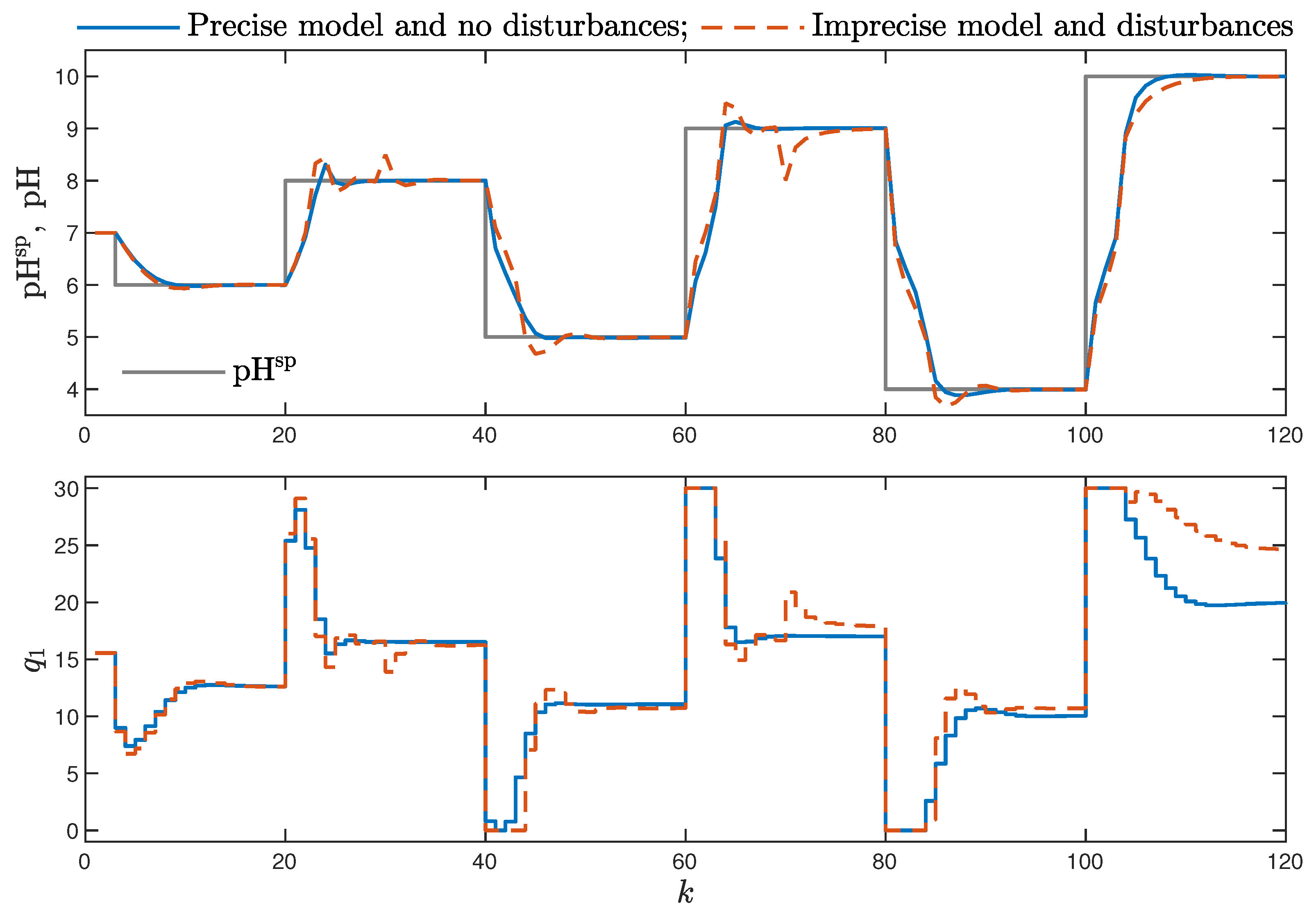
In the first case, the model utilised in MPC is precise and no external disturbances occur. Let us stress that the model is precise but not perfect, i.e., there is always some model error. The simulation model and the model used in MPC have different structures, i.e., a set of differential equations and a Wiener structure, respectively.

2.

In the second case, the model is imperfect and disturbances affect the process. The following model imperfection is considered: the steady-state model gain is decreased by 25%. As far as the disturbance scenario is concerned, two unmeasured step disturbances that act on the process output are used. The first of them is activated at $k=30$ and it has the value 0.5, the second one is activated at $k=70$ and it has the value $-0.5$.

In all simulations, the MPC controller has the same tuning parameters. The prediction horizon (N) is 10, the control horizon ($N_{\mathrm{u}}$) is 5 and the penalty quotient $\lambda$ is 0.1. As tuning of MPC is standard textbook material [1,2,3], this issue is not considered in this work. The magnitude of the manipulated process input variable is limited: $q_1^{min}=0$, $q_1^{max}=30$. MATLAB is used to perform all simulations. The fmincon function is used for nonlinear optimisation, whereas the quadprog function is used for solving auxiliary MPC quadratic tasks in initialisation strategies 11 and 12. Figure 1 depicts the trajectories of the manipulated and controlled variables for a series of set-point changes. Of note, the MPC algorithm has an integral action, similarly to the classical PID controller, since an imperfect model and disturbances do not result in a steady-state error.

At first, simple strategies 1–5 are considered. The results are given in

Table 1. The SISO process (precise model and no disturbances) for simple strategies 1–5: the number of cost-function evaluations and the time of calculation.

Strategy	Cost-Function Evaluations (%)	Calculation Time (%)
1	96.9 ${}^{*}$	97.4
2	92.9${}^{\phantom{*}}$	93.1
3	100.0${}^{\phantom{*}}$	100.0
4	71.8${}^{\phantom{*}}$	76.1
5	59.9${}^{\phantom{*}}$	65.6

* The average value, the range is 95.3–99.2%.

and

Table 2. The SISO process (imprecise model and disturbances) for simple strategies 1–5: the number of cost-function evaluations and the time of calculation.

Strategy	Cost-Function Evaluations (%)	Calculation Time (%)
1	91.2 ${}^{**}$	91.2
2	82.4${}^{\phantom{**}}$	84.2
3	90.9${}^{\phantom{**}}$	91.6
4	72.2${}^{\phantom{**}}$	75.6
5	63.3${}^{\phantom{**}}$	68.4

** The average value, the range is 90.6–91.9%.

for two cases of model accuracy and disturbances. For each of the considered strategies, the total number of cost-function evaluations and the calculation time are specified; both measures are scaled to provide hardware-independent results. Since the initial vector is chosen randomly in the case of strategy 1, five runs are performed. The following observations are possible:

1.

In the case of random strategy 1, interestingly, variability in the number of cost-function evaluations is quite low.

2.

Strategy 3 (the initial vector is in the centre of the set determined by the linear constraints imposed on the magnitude of the manipulated variable) turns out to be most inefficient both in terms of the cost-function evaluations and the calculation time.

3.

Random strategy 1 is slightly better, strategy 2 (all elements of the initial vector are 0) is better, strategy 4 (the initial vector is set to the vector of manipulated variables calculated and utilised at the previous sampling instant) is better and strategy 5 (the initial vector is the “tail” of the optimal control sequence from the previous sampling instant) is the best one.

As far as assessing the influence of model inaccuracy and the external disturbance on the computational burden is concerned, we observe that:

1.

For the chosen model inaccuracy and disturbances scenario, strategy 1 needs slightly fewer function evaluations when the model is imprecise and disturbances occur, but, in general, the opposite may also be true.

2.

A similar phenomenon is observed for strategies 2 and 3. Conversely, in the case of strategies 4 and 5, the function evaluation numbers are very similar for the two considered scenarios. The explanation of this phenomenon is straightforward: strategies 1, 2 and 3 do not take into account the current process operating point for initialisation of the MPC optimisation task.

3.

The simpler strategy 4 which relies only on the values of the process inputs applied at the previous sampling instant gives noticeably worse results than strategy 5 in which the part of the last optimal solution is utilised.

Next, let us discuss the results given by strategies 6 and 7. In this work, we consider the linear approximator (11) and the neural one (12). We consider three configurations of the approximator’s input (Equation (10)): in the first case, $n_{\mathrm{A}}=0$, $n_{\mathrm{B}}=0$, hence

$$\mathit{x}\left(k\right)={\left[y\left(k\right)y^{\mathrm{sp}}\left(k\right)\right]}^{\mathrm{T}}$$

(24)

in the second case, $n_{\mathrm{A}}=1$, $n_{\mathrm{B}}=1$, hence

$$\mathit{x}\left(k\right)={\left[u(k-1)y\left(k\right)y(k-1)y^{\mathrm{sp}}\left(k\right)\right]}^{\mathrm{T}}$$

(25)

in the third case, $n_{\mathrm{A}}=2$, $n_{\mathrm{B}}=2$, hence

$$\mathit{x}\left(k\right)={\left[u(k-1)u(k-2)y\left(k\right)y(k-1)y(k-2)y^{\mathrm{sp}}\left(k\right)\right]}^{\mathrm{T}}$$

(26)

The classical neural network with one hidden layer containing K hidden nodes of the tanh type and a linear output is used as the neural approximator. For identification of linear and neural approximators (training), 5000 data samples for different operating conditions of the process are used. The available set is randomly divided into three parts: the training set consists of 3000 samples, the validation and test sets are comprised of 1000 samples, respectively. The classical least squares method is used to identify the linear approximator. For training of the neural approximators, the Levenberg–Marquardt algorithm is used.

Table 3. The SISO process: accuracy of linear and neural approximators in terms of MSE errors.

Approximator	Arguments	Parameters	${\mathrm{MSE}}_{\mathbf{train}}$	${\mathrm{MSE}}_{\mathbf{val}}$	${\mathrm{MSE}}_{\mathbf{test}}$
Linear	Equation (24)	15	5.3373 $\times {10}^{-3}$	4.9654 $\times {10}^{-3}$	4.9513 $\times {10}^{-3}$
Neural, $K=5$		45	1.2773 $\times {10}^{-3}$	1.3381 $\times {10}^{-3}$	1.0132 $\times {10}^{-3}$
Neural, $K=10$		85	7.3032 $\times {10}^{-4}$	7.2437 $\times {10}^{-4}$	6.0605 $\times {10}^{-4}$
Neural, $K=15$		125	5.4709 $\times {10}^{-4}$	5.1918 $\times {10}^{-4}$	4.9427 $\times {10}^{-4}$
Neural, $K=20$		165	4.5691 $\times {10}^{-4}$	4.3918 $\times {10}^{-4}$	4.4869 $\times {10}^{-4}$
Neural, $K=25$		205	4.1833 $\times {10}^{-4}$	4.5292 $\times {10}^{-4}$	4.3530 $\times {10}^{-4}$
Neural, $K=30$		245	3.9074 $\times {10}^{-4}$	4.2546 $\times {10}^{-4}$	4.3211 $\times {10}^{-4}$
Linear	Equation (25)	25	3.6782 $\times {10}^{-3}$	3.3738 $\times {10}^{-3}$	3.4537 $\times {10}^{-3}$
Neural, $K=5$		55	7.2419 $\times {10}^{-4}$	6.6889 $\times {10}^{-4}$	5.8716 $\times {10}^{-4}$
Neural, $K=10$		105	2.9651 $\times {10}^{-4}$	3.3246 $\times {10}^{-4}$	2.7288 $\times {10}^{-4}$
Neural, $K=15$		155	1.8590 $\times {10}^{-4}$	2.3223 $\times {10}^{-4}$	1.4656 $\times {10}^{-4}$
Neural, $K=20$		205	1.4377 $\times {10}^{-4}$	1.8215 $\times {10}^{-4}$	1.3796 $\times {10}^{-4}$
Neural, $K=25$		255	9.6805 $\times {10}^{-5}$	1.2252 $\times {10}^{-4}$	9.4940 $\times {10}^{-5}$
Neural, $K=30$		305	6.8775 $\times {10}^{-5}$	1.0455 $\times {10}^{-4}$	9.1554 $\times {10}^{-5}$
Linear	Equation (26)	35	3.5254 $\times {10}^{-3}$	3.2598 $\times {10}^{-3}$	3.3680 $\times {10}^{-3}$
Neural, $K=5$		65	1.1606 $\times {10}^{-3}$	1.1889 $\times {10}^{-3}$	9.4163 $\times {10}^{-4}$
Neural, $K=10$		125	3.2301 $\times {10}^{-4}$	3.5967 $\times {10}^{-4}$	2.7965 $\times {10}^{-4}$
Neural, $K=15$		185	1.7700 $\times {10}^{-4}$	2.0761 $\times {10}^{-4}$	1.3671 $\times {10}^{-4}$
Neural, $K=20$		245	1.0715 $\times {10}^{-4}$	1.4289 $\times {10}^{-4}$	1.1296 $\times {10}^{-4}$
Neural, $K=25$		305	8.8876 $\times {10}^{-5}$	1.3037 $\times {10}^{-4}$	9.2147 $\times {10}^{-5}$
Neural, $K=30$		365	5.4820 $\times {10}^{-5}$	1.1215 $\times {10}^{-4}$	7.5876 $\times {10}^{-5}$

shows accuracy of linear and neural approximators in terms of the mean squared error (MSE), i.e., the sum of squared errors for all data samples divided by the number of samples. Additionally, the number of approximators’ parameters is specified. The approximators with three different input vectors, defined by Equations (24)–(26), respectively, are considered. Each configuration of the neural approximator is trained as many as ten times and only the best results are presented in this work. All approximators are assessed taking into account the error for the validation data set, which is not used during training. From Table 3 we may find out that:

1.

In general, the approximators that determine the initial point for MPC optimisation as the function of only the current values of the set-point and process output (i.e., their arguments are defined by Equation (24)) have low quality.

2.

The approximators that additionally take into account the values of process manipulated and controlled variables from the previous sampling instant (Equation (25)) are characterised by significantly lower errors.

3.

Further lengthening of the vector $\mathit{x}\left(k\right)$ as in Equation (26) does not improve the resulting approximators’ accuracy much.

4.

The linear approximators have large errors while the errors of the neural ones are much lower. Of course, the more the hidden nodes K, the lower the approximation errors.

Figure 2 demonstrates the relation between the validation data set and the output of linear and neural approximators with 5, 10, 15, 20, 25 and 30 hidden nodes; all approximators use the input vector defined by Equation (25). We may assess that the neural approximator should be used rather than the imprecise linear one. Moreover, the neural approximator with only five hidden nodes should also be avoided. Of course, the higher the number of hidden nodes, the better the approximation accuracy.

Table 4. The SISO process (precise model and no disturbances) for approximator-based strategies 6 and 7: the number of cost-function evaluations and the calculation time.

Strategy	Approximator	Cost-Function Evaluations (%)	Calculation Time (%)
6	Linear, arguments (25)	69.8	74.2
6	Neural, $K=10$, arguments (25)	64.3	69.6
6	Neural, $K=20$, arguments (25)	62.1	67.5
6	Neural, $K=30$, arguments (25)	62.0	67.9
6	Linear, arguments (26)	69.5	67.9
6	Neural, $K=10$, arguments (26)	64.4	69.7
6	Neural, $K=20$, arguments (26)	61.8	67.1
6	Neural, $K=30$, arguments (26)	61.0	66.7
7	Neural, $K=20$, arguments (25)	58.7	64.8

and

Table 5. The SISO process (imprecise model and disturbances) for approximator-based strategies 6 and 7: the number of cost-function evaluations and the calculation time.

Strategy	Approximator	Cost-Function Evaluations (%)	Calculation Time (%)
6	Linear, arguments (25)	74.5	78.3
6	Neural, $K=10$, arguments (25)	75.5	78.9
6	Neural, $K=20$, arguments (25)	76.2	80.0
6	Neural, $K=30$, arguments (25)	77.2	80.4
6	Linear, arguments (26)	74.1	78.1
6	Neural, $K=10$, arguments (26)	76.0	79.5
6	Neural, $K=20$, arguments (26)	75.3	79.3
6	Neural, $K=30$, arguments (26)	76.7	80.6
7	Neural, $K=20$, arguments (25)	63.3	68.8

present effectiveness of MPC initialisation strategy 6, i.e., the scaled total number of cost-function evaluations and the scaled calculation time are specified; two cases of model accuracy and disturbances are considered. We find out that:

1.

In general, we can observe that the higher the number of hidden nodes, the lower the number of cost-function evaluations, but 20 hidden nodes seem to be completely sufficient.

2.

Furthermore, there is no point in using the longest vector of approximators’ input given by Equation (26), it is sufficient to use the inputs defined by Equation (25).

3.

Taking into account Table 1 and Table 2, it is very interesting to note that all neural approximators lead to significantly lower numbers of cost-function evaluation than the simple initialisation strategies 1–3 and noticeable lower numbers possible in the case of strategy 4, but only when the model is accurate and no disturbances occur.

4.

When the model is imprecise and disturbances are present, the linear and neural approximators give noticeable higher numbers of cost-function evaluations. When the approximators are used, all results are worse when compared with those obtained when initialisation strategy 5 is applied; this observation is true in both model accuracy and disturbances cases. Hence, we find out that the pure approximation of the initial solution to MPC is not robust when the properties of the model change and there are unexpected disturbances (i.e., the results for two considered models of model accuracy and disturbances are very different).

5.

Initialisation strategy 7, which is a combination of strategies 5 and 6, gives really good results, much better than the pure strategy 6. We can observe that strategy 7 is quite robust to model errors and disturbances that affect the controlled process.

Efficiency of the inverse model-based initialisation strategy 8 and hybrid strategies 9–12 is compared in

Table 6. The SISO process (precise model and no disturbances) for hybrid strategies 8–12: the number of cost-function evaluations and the calculation time.

Strategy	Cost-Function Evaluations (%)	Calculation Time (%)
8	70.9	75.5
9	83.3	86.0
10	56.0	63.1
11	83.7	98.8
12	56.0	76.0

and

Table 7. The SISO process (imprecise model and disturbances) for hybrid strategies 8–12: the number of cost-function evaluations and the calculation time.

Strategy	Cost-Function Evaluations (%)	Calculation Time (%)
8	81.1	83.6
9	86.9	89.1
10	55.7	63.4
11	85.3	101.5
12	54.9	75.4

in terms of the numbers of the cost-function evaluations and the calculation time. We can draw the following conclusions:

1.

Strategy 8, which uses an inverse static model and the current value of the set-point, is quite inefficient, in particular, for the imprecise model and disturbances.

2.

Hybrid strategies 9 and 11, in which an auxiliary MPC controller based on a fully linear model is used, give bad results. They are robust to model imperfections and disturbances, but, generally, many cost-function evaluations are necessary in nonlinear MPC. It is because a very rough linear representation of the nonlinear process is used in the auxiliary MPC. The results are poor no matter if the auxiliary controller is the explicit one (strategy 9) or quadratic optimisation is used (strategy 11).

3.

Excellent results, the best of all compared in terms of the number of the cost-function evaluation, are obtained when strategies 10 and 12 are used. The auxiliary MPC controller uses a time-varying linear representation of the nonlinear process. The future control policy determined by such a controller, when used as the initial point in the nonlinear MPC optimisation, needs the lowest number of the cost-function evaluation. Taking into consideration the calculation time, it is evident that it is better to use strategy 10 in which an explicit auxiliary MPC controller is used rather than the more time-consuming quadratic optimisation necessary in strategy 12. The explicit controller is sufficient for the simple box constraints used in this study.

4.

Two further advantages of strategy 10 (and strategy 12) must be stressed. Firstly, they need a significantly lower number of the cost-function evaluations than all simple strategies 1–5, the approximator based strategies 6 and 7 as well as the inverse model-based strategy 8. Even strategy 5, i.e., the use of the “tail” of the previous optimal sequence, is slightly worse. Secondly, strategies 10 and 12 prove to be very robust to model errors and process disturbances. The only drawback of strategies 10 and 12 is that the calculation time is significantly longer than the one needed when strategy 5 is used.

5.

Strategies 10 and 12 are the best in terms of the need for the cost-function evaluations. However, in their case, the calculation time is considerably larger than in the case of strategy 5. Unfortunately, this problem grows with the number of decision variables in the optimisation problem solved at each iteration of the MPC algorithm. Therefore, in the case of multivariable control plants, strategy 5 seems to offer the best solution to minimise the energy consumption needed to solve the MPC optimisation task.

For the neutralisation reactor, initialisation strategy 10 that uses an auxiliary explicit MPC controller with successive model linearisation performs best. Nevertheless, simple strategy 5 that uses the part of the optimal solution from the previous sampling instant gives only slightly worse results. Both strategies are robust to model errors and disturbances.

6.2. MIMO Process: Robot Manipulator

The second considered process is 7DOF KUKA LWR 4+ robot arm [59] mounted on a rotating torso (column). It is a multivariable control plant; the manipulated inputs are joint torque residuals after gravity removal ${\tau }_{\mathrm{g},i}$, $i=2,\dots ,8$; the controlled outputs are three components of the position of the end effector $x_{\mathrm{ce}}$, $y_{\mathrm{ce}}$, $z_{\mathrm{ce}}$, and the constrained outputs are joint angles $q_i$, $i=2,\dots ,8$. It is assumed that the column is not moved (${\tau }_{\mathrm{g},\mathrm{col}}=0$).

The full model of the robot is implemented in the open-source robot simulator environment Gazebo [60]. It is based on differential equations motivated by physical laws. In MPC, the simplified model of the control plant is used. It has the Hammerstein–Wiener structure, i.e., a dynamic block is surrounded by two static blocks; a static block preceding the dynamic block realises gravity compensation, and the static block following the dynamic block calculates forward kinematics for the end effector. Such a model has been derived from analysis of reactions of the full model available in Gazebo and behaviour of the real process. The sampling time of the MPC model and the MPC arm algorithm is 50 ms.

The limitations related to the magnitude of the manipulated variables are

$$\begin{array}{cccc}\hfill {\tau }_{\mathrm{g},2}^{min}& =-88,\hfill & \hfill {\tau }_{\mathrm{g},2}^{max}& =88,\hfill \\ \hfill {\tau }_{\mathrm{g},3}^{min}& =-88,\hfill & \hfill {\tau }_{\mathrm{g},3}^{max}& =88,\hfill \\ \hfill {\tau }_{\mathrm{g},4}^{min}& =-50,\hfill & \hfill {\tau }_{\mathrm{g},4}^{max}& =50,\hfill \\ \hfill {\tau }_{\mathrm{g},5}^{min}& =-50,\hfill & \hfill {\tau }_{\mathrm{g},5}^{max}& =50,\hfill \\ \hfill {\tau }_{\mathrm{g},6}^{min}& =-50,\hfill & \hfill {\tau }_{\mathrm{g},6}^{max}& =50,\hfill \\ \hfill {\tau }_{\mathrm{g},7}^{min}& =-19,\hfill & \hfill {\tau }_{\mathrm{g},7}^{max}& =19,\hfill \\ \hfill {\tau }_{\mathrm{g},8}^{min}& =-19,\hfill & \hfill {\tau }_{\mathrm{g},8}^{max}& =19\hfill \end{array}$$

(27)

The constraints imposed on the joint angles are

$$\begin{array}{cccc}\hfill q_2^{min}& =-154,\hfill & \hfill q_2^{max}& =154,\hfill \\ \hfill q_3^{min}& =-104,\hfill & \hfill q_3^{max}& =-26,\hfill \\ \hfill q_4^{min}& =-154,\hfill & \hfill q_4^{max}& =154,\hfill \\ \hfill q_5^{min}& =26,\hfill & \hfill q_5^{max}& =104,\hfill \\ \hfill q_6^{min}& =-154,\hfill & \hfill q_6^{max}& =154,\hfill \\ \hfill q_7^{min}& =-104,\hfill & \hfill q_7^{max}& =-26,\hfill \\ \hfill q_8^{min}& =-154,\hfill & \hfill q_8^{max}& =154\hfill \end{array}$$

(28)

The horizons used in MPC are: $N=25$, $N_{\mathrm{u}}=5$, which means that the MPC optimisation task has 35 decision variables. It is a fundamental change compared with the much simpler neutralisation reactor case with only five decision variables.

Taking into account the results obtained for the neutralisation process, strategies 1 (the random initialisation), 4 (the vector of manipulated process inputs determined and applied to the process at the previous sampling instant is used) and 5 (the initial vector is formed using the “tail” of the optimal control sequence from the previous sampling instant) are chosen for comparison in the case of the robot. It is because they are simple, yet the last of them is expected to be efficient. As many as 20 simulations for each initialisation strategy are performed, consisting of one set-point change, i.e., movement of the manipulator to a different position. 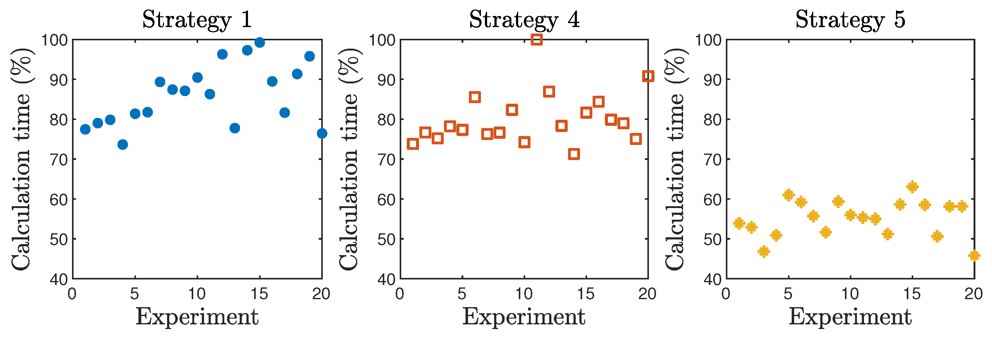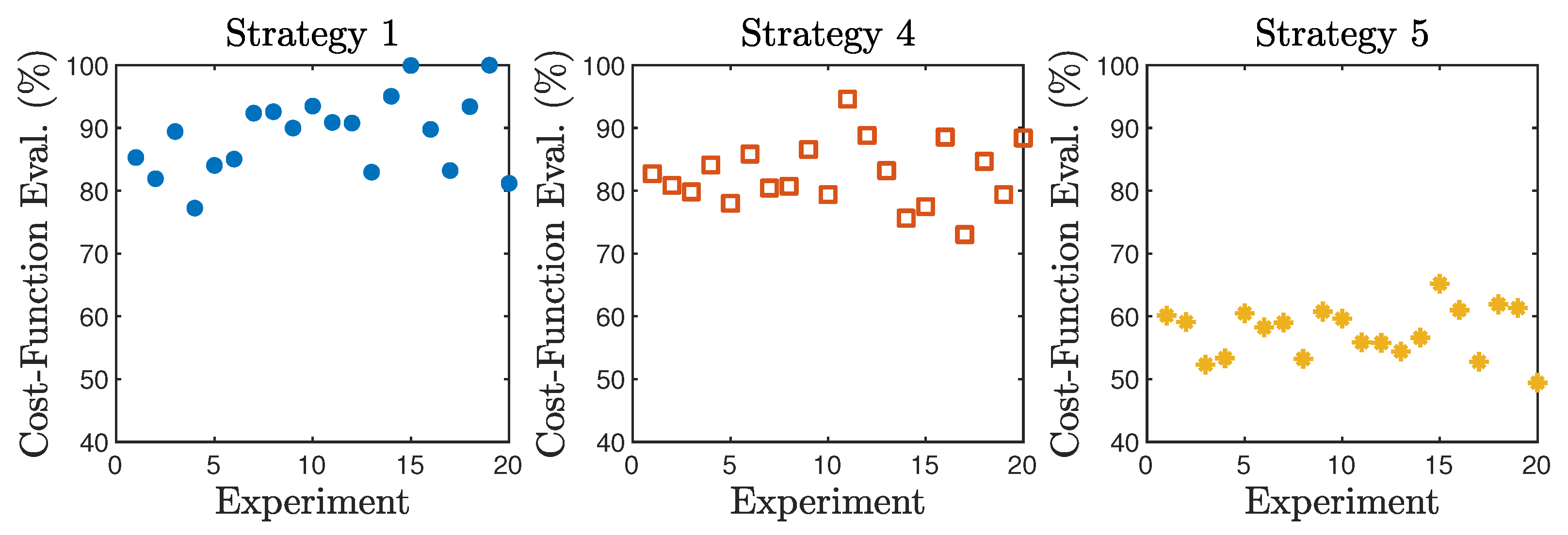Figure 3 and Figure 4 depict the scaled number of MPC cost-function evaluations and the scaled time of calculation of MPC in the consecutive 20 simulations. Moreover,

Table 8. The MIMO process for initialisation strategies 1, 4 and 5: the average number of cost-function evaluations and the calculation time in the consecutive 20 simulations.

Strategy	Cost-Function Evaluations (%)	Calculation Time (%)
1	100.0	100.0
4	92.9	93.3
5	64.7	64.1

reports average values of these performance indicators for all simulations. We can draw the following observations.

1.

In terms of two considered indicators, initialisation method 1 is the worst one, method 4 gives slightly better results and strategy 5 is the best one. It is important that strategy 5 is much better than strategy 4; the relation ismuch more favourable than the comparison between strategies 1 and 4, respectively.

2.

Of note, variability of the number of cost-function evaluations and the calculation time is larger in the case of initialisation methods 1 and 4 when compared with strategy 5.

3.

When compared with the results obtained for the neutralisation reactor (Table 1), despite that in two considered benchmark processes the number of process input and output variables as well as the length of the optimised MPC decision vector are different, the results are quite similar.

We can see that efficiency of methods 1, 4 and 5 is similar for both the SISO neutralisation reactor and MIMO process, as shown in Table 1, Table 2 and Table 8. It is crucial since the recommended method 5 can be applied for different processes, with different properties and the number of inputs and outputs. It is evident that method 1 is the worst one, method 4 is slightly better and strategy 5 is significantly better. Hybrid methods 10 and 11 are not available for the MIMO case but, bearing in mind the results obtained for the SISO process (Table 6 and Table 7), method 5 is only slightly slower than the hybrid methods, yet much simpler.

7. Discussion of Obtained Results and Properties of the Initialisation Strategies

Among the classical initialisation methods, strategy 5, which uses the “tail” of the optimal solution found at the previous sampling instant, is the best in terms of the cost-function evaluations and the time of calculation. It is necessary to stress that the method works very well when disturbances affect the process and its parameters change.

Approximator-based methods 6, 7 and inverse model-based method 8 give fairly good results in terms of both considered quality indicators only in the nominal model case. Unfortunately, their efficiency decreases when the model imperfections are present and process disturbances occur.

As far as the hybrid methods are concerned, methods 10 and 12, which use an auxiliary MPC controller with a successively linearised model, are the best in terms of the calculation time and the cost-function evaluations. Moreover, strategy 10 is faster because the solution to the auxiliary MPC problem is obtained analytically, without any on-line optimisation. Methods 9 and 11 are worse since a parameter-constant linear model is used in the auxiliary MPC task. Importantly, all hybrid methods are very robust when the process is disturbed and the model is not precise.

Let us shortly discuss the universal properties of the defined strategies. Simple methods 1–5 do not use any model or approximator, while methods 6–12 rely on different models. However, the approximator used in methods 6 or 7 is not the same or a simplified version of the dynamical model used in MPC; it simply attempts to approximate the solution to the MPC optimisation task using a set of historical data. Similarly, the inverse static model used in strategy 8 is not the same as the model used in MPC. The authors’ hybrid methods 9–12 are significantly different since for initialisation of the nonlinear MPC optimisation task, a simplified MPC optimisation task is formulated and solved. The differences between the hybrid methods described result from using a different model simplification approach for the auxiliary controller and the way its optimisation task is solved. A constant linear model is used in strategies 9 and 11, while a time-varying one is used in methods 10 and 12. Furthermore, the auxiliary controller utilises an explicit solution in strategies 9 and 10, while quadratic optimisation is used in strategies 11 and 12.

Because a simplified version of the nonlinear model (used in the nonlinear MPC algorithm) is used in the auxiliary controller, the hybrid methods have two important advantages over all other methods. Firstly, the auxiliary controller has a negative feedback mechanism, the same that is used in the nonlinear MPC algorithm. It means that all model errors and disturbances affecting the process are compensated for during calculation performed by the auxiliary controller. Such a mechanism is not present in all other methods. Secondly, the auxiliary and nonlinear MPC algorithms solve the same optimisation task but using different models and methods. It also means that if we develop a nonlinear MPC algorithm, we can use the hybrid methods as well, provided we can obtain simple linear or linearised versions of the full nonlinear model the MPC algorithm is based on.

Of note, the sophisticated approximator-based methods 6 and 7 do not offer any feedback mechanism. As a result, one may train a perfect approximator for historical data, but it is likely to give poor results when properties of the process are time-varying or important disturbances occur in the control system. The inverse model-based method suffers from the same shortcoming.

It is important to discuss the influence of the number of process inputs and outputs on efficiency of the compared initialisation methods. Firstly, concerning the results of simulation experiments of the MIMO process discussed in Section 6.2, strategy 5 is very efficient in terms of both quality indicators. The same result is obtained for the SISO plant. Secondly, approximator-based methods 6, 7 and inverse model-based method 8 require much more complicated models when the number of process signals and model parameters increases. Thirdly, hybrid methods 9 and 10 based on explicit auxiliary MPC controllers are very efficient because the initial vector is calculated from an analytical formula; on-line optimisation is avoided. Conversely, methods 11 and 12 require auxiliary quadratic optimisation, which takes much more time to find the solution, particularly when many process variables are used.

8. Conclusions

The choice of the initialisation strategies for the nonlinear MPC optimisation task greatly influences the number of cost-function evaluations and the necessary calculation time. Efficiency of twelve initialisation methods is thoroughly discussed for a neutralisation reactor benchmark process. It is found out that:

1.

Simple strategies 1, 2 and 3 do not take into account any information of the current set-point and the process operating point. As a result, their effectiveness is very low.

2.

Strategies 4 and 5 do not use the current set-point but do use the current operating point. Simple strategy 4, in which the value of the process inputs from the previous sampling instant is used, gives much better results than simple strategies 1, 2 and 3. Strategy 5, in which the “tail” of the optimal control sequence from the previous sampling instant is used, gives excellent results.

3.

Approximator-based methods 6 and 7 (in this work, a neural approximator is used) are quite complex since they need to be sufficiently collecting sets of data and training an approximator. Unfortunately, their performance is good (comparable to method 5) only for the precise model case. When model errors and disturbances occur, method 5 outperforms the approximator-based methods.

4.

Inverse model-based method 8 requires an additional static model which for some processes may be not available. Unfortunately, since the method does not use the current operating point, it is not very efficient, in particular, for the imprecise model and disturbances.

5.

The authors’ original hybrid methods 11 and 12 are fairly complicated as they require solving an auxiliary quadratic programming problem at each sampling instant. The authors’ methods 9 and 10 are much simpler since an analytical auxiliary controller is utilised. Method 10, in which a linear approximation of the nonlinear model is determined on-line to be used in the auxiliary controller, is the fastest one. It must be pointed out that strategy 10 works very well for the imperfect model and disturbances. Since a simplified version of the model is used in the auxiliary controller, the hybrid methods perform much better than the approximation-based ones with complex neural networks. The auxiliary controller has a negative feedback mechanism to compensate model errors and disturbances.

We find out that methods 5 and 10 are the fastest ones and are robust to model inaccuracies and disturbances. Strategy 10 is slightly better than 5. However, the difference is not significant, but method 10 is much more complicated.

All things considered, when the auxiliary MPC controller based on a successively linearised model is available, it may be successfully used for initialisation of nonlinear MPC. Although much simpler, the method based on the part of the optimal solution obtained at the previous sampling instant also gives excellent results. Unfortunately, quite sophisticated methods based on a neural approximator are very disappointing.

In future research, it is worth trying to improve the initialisation methods based on neural approximators. In particular, it would be necessary to reduce or eliminate the fundamental weakness of approximator-based methods, which is the lack of robustness to disturbances and process changes.

References

- Camacho, E.F.; Bordons, C. Model Predictive Control; Springer: London, UK, 1999. [Google Scholar]
- Maciejowski, J. Predictive Control with Constraints; Prentice Hall: Harlow, UK, 2002. [Google Scholar]
- Tatjewski, P. Advanced Control of Industrial Processes, Structures and Algorithms; Springer: London, UK, 2007. [Google Scholar]
- Nebeluk, R.; Marusak, P. Efficient MPC algorithms with variable trajectories of parameters weighting predicted control errors. Arch. Control Sci. 2020, 30, 325–363. [Google Scholar]
- Assandri, A.D.; de Prada, C.; Rueda, A.; Martínez, J.S. Nonlinear parametric predictive temperature control of a distillation column. Control Eng. Pract. 2013, 21, 1795–1806. [Google Scholar] [CrossRef]
- Sheik, A.G.; Tejaswini, E.; Seepana, M.M.; Ambati, S.R.; Meneses, M.; Vilanova, R. Design of feedback control strategies in a plant-wide wastewater treatment plant for simultaneous evaluation of economics, energy usage, and removal of nutrients. Energies 2021, 14, 6386. [Google Scholar] [CrossRef]
- Ogonowski, S.; Bismor, D.; Ogonowski, Z. Control of complex dynamic nonlinear loading process for electromagnetic mill. Arch. Control Sci. 2020, 30, 471–500. [Google Scholar]
- Castañeda, L.Á.; Guzman-Vargas, L.; Chairez, I.; Luviano-Juárez, A. Output based bilateral adaptive control of partially known robotic systems. Control Eng. Pract. 2020, 98, 104362. [Google Scholar] [CrossRef]
- Sánchez, A.; Gallego, A.; Escaño, J.; Camacho, E. Adaptive incremental state space MPC for collector defocusing of a parabolic trough plant. Sol. Energy 2019, 184, 105–114. [Google Scholar] [CrossRef]
- Sawant, P.; Villegas Mier, O.; Schmidt, M.; Pfafferott, J. Demonstration of optimal scheduling for a building heat pump system using economic-MPC. Energies 2021, 14, 7953. [Google Scholar] [CrossRef]
- Garcia-Torres, F.; Valverde, L.; Bordons, C. Optimal Load Sharing of Hydrogen-Based Microgrids with Hybrid Storage Using Model-Predictive Control. IEEE Trans. Ind. Electron. 2016, 63, 4919–4928. [Google Scholar] [CrossRef]
- Gruber, J.K.; Bordons, C.; Oliva, A. Nonlinear MPC for the airflow in a PEM fuel cell using a Volterra series model. Control Eng. Pract. 2012, 20, 205–217. [Google Scholar] [CrossRef]
- Zhao, J.; Hu, Y.; Xie, F.; Li, X.; Sun, Y.; Sun, H.; Gong, X. Modeling and integrated optimization of power split and exhaust thermal management on diesel hybrid electric vehicles. Energies 2021, 14, 7505. [Google Scholar] [CrossRef]
- Musa, A.; Pipicelli, M.; Spano, M.; Tufano, F.; De Nola, F.; Di Blasio, G.; Gimelli, A.; Misul, D.A.; Toscano, G. A review of model predictive controls applied to advanced driver-assistance systems. Energies 2021, 14, 7974. [Google Scholar] [CrossRef]
- Chanfreut, P.; Maestre, J.M.; Camacho, E. Coalitional model predictive control on freeways traffic networks. IEEE Trans. Intell. Transp. Syst. 2019, 22, 6772–6783. [Google Scholar] [CrossRef]
- Bania, P. An information based approach to stochastic control problems. Int. J. Appl. Math. Comput. Sci. 2020, 30, 47–59. [Google Scholar]
- Huang, Y.; Wang, H.; Khajepour, A.; He, H.; Ji, J. Model predictive control power management strategies for HEVs: A review. J. Power Sources 2017, 341, 91–106. [Google Scholar] [CrossRef]
- Hu, J.; Shan, Y.; Guerrero, J.M.; Ioinovici, A.; Chan, K.W.; Rodriguez, J. Model predictive control of microgrids—An overview. Renew. Sustain. Energy Rev. 2021, 136, 110422. [Google Scholar] [CrossRef]
- Borhan, H.; Vahidi, A.; Phillips, A.M.; Kuang, M.L.; Kolmanovsky, I.V.; Di Cairano, S. MPC–Based Energy Management of a Power–Split Hybrid Electric Vehicle. IEEE Trans. Control Syst. Technol. 2012, 20, 593–603. [Google Scholar] [CrossRef]
- Zhang, S.; Zhuan, X. Model–Predictive Optimization for Pure Electric Vehicle during a Vehicle–Following Process. Math. Probl. Eng. 2019, 2019, 5219867. [Google Scholar] [CrossRef]
- Ji, Z.; Huang, X.; Xu, C.; Sun, H. Accelerated Model Predictive Control for Electric Vehicle Integrated Microgrid Energy Management: A Hybrid Robust and Stochastic Approach. Energies 2016, 9, 973. [Google Scholar] [CrossRef]
- Ryu, K.S.; Kim, D.J.; Ko, H.; Boo, C.J.; Kim, J.; Jin, Y.G.; Kim, H.C. MPC Based Energy Management System for Hosting Capacity of PVs and Customer Load with EV in Stand-Alone Microgrids. Energies 2021, 14, 4041. [Google Scholar] [CrossRef]
- Choi, B.R.; Lee, W.P.; Won, D.J. Optimal Charging Strategy Based on Model Predictive Control in Electric Vehicle Parking Lots Considering Voltage Stability. Energies 2018, 11, 1812. [Google Scholar] [CrossRef] [Green Version]
- Ghotge, R.; Snow, Y.; Farahani, S.; Lukszo, Z.; van Wijk, A. Optimized Scheduling of EV Charging in Solar Parking Lots for Local Peak Reduction under EV Demand Uncertainty. Energies 2020, 13, 1275. [Google Scholar] [CrossRef] [Green Version]
- Hajar, K.; Hably, A.; Bacha, S.; Elrafhi, A.; Obeid, Z. An application of a centralized model predictive control on microgrids. In Proceedings of the 2016 IEEE Electrical Power and Energy Conference (EPEC), Ottawa, ON, Canada, 12–14 October 2016; pp. 1–6. [Google Scholar]
- Yan, F.; Wang, J.; Huang, K. Hybrid Electric Vehicle Model Predictive Control Torque-Split Strategy Incorporating Engine Transient Characteristics. IEEE Trans. Veh. Technol. 2012, 61, 2458–2467. [Google Scholar] [CrossRef]
- Santucci, A.; Sorniotti, A.; Lekakou, C. Power split strategies for hybrid energy storage systems for vehicular applications. J. Power Sources 2014, 258, 395–407. [Google Scholar] [CrossRef] [Green Version]
- Josevski, M.; Abel, D. Energy Management of Parallel Hybrid Electric Vehicles based on Stochastic Model Predictive Control. IFAC Proc. Vol. 2014, 47, 2132–2137. [Google Scholar] [CrossRef] [Green Version]
- Koot, M.; Kessels, J.; de Jager, B.; Heemels, W.; van den Bosch, P.; Steinbuch, M. Energy management strategies for vehicular electric power systems. IEEE Trans. Veh. Technol. 2005, 54, 771–782. [Google Scholar] [CrossRef]
- Debert, M.; Yhamaillard, G.; Ketfi-herifellicaud, G.A. Predictive energy management for hybrid electric vehicles—Prediction horizon and battery capacity sensitivity. IFAC Proc. Vol. 2010, 43, 270–275. [Google Scholar] [CrossRef] [Green Version]
- Li, S.E.; Jia, Z.; Li, K.; Cheng, B. Fast online computation of a model predictive controller and its application to fuel economy-oriented adaptive cruise control. IEEE Trans. Ind. Informat. 2015, 16, 1199–1209. [Google Scholar] [CrossRef]
- Fruzzetti, K.P.; Palazoğlu, A.; McDonald, K.A. Nonlinear model predictive control using Hammerstein models. J. Process Control 1997, 7, 31–41. [Google Scholar] [CrossRef]
- Cervantes, A.L.; Agamennoni, O.E.; Figueroa, J.L. A nonlinear model predictive control system based on Wiener piecewise linear models. J. Process Control 2003, 13, 655–666. [Google Scholar] [CrossRef]
- Norquay, S.J.; Palazoğlu, A.; Romagnoli, J. Application of Wiener model predictive control (WMPC) to an industrial C2 splitter. J. Process Control 1999, 9, 461–473. [Google Scholar]
- Shafiee, G.; Arefi, M.M.; Jahed-Motlagh, M.R.; Jalali, A.A. Nonlinear predictive control of a polymerization reactor based on piecewise linear Wiener model. Chem. Eng. J. 2008, 143, 282–292. [Google Scholar] [CrossRef]
- Ding, B.; Ping, X. Dynamic output feedback model predictive control for nonlinear systems represented by Hammerstein-Wiener model. J. Process Control 2012, 22, 1773–1784. [Google Scholar] [CrossRef]
- Hong, M.; Cheng, S. Hammerstein-Wiener model predictive control of continuous stirred tank reactor. In Electronics and Signal Processing; Hu, W., Ed.; Lecture Notes in Electric Engineering; Springer: Berlin/Heidelberg, Germany, 2011; Volume 97, pp. 235–242. [Google Scholar]
- Ławryńczuk, M. Nonlinear Predictive Control Using Wiener Models: Computationally Efficient Approaches for Polynomial and Neural Structures; Studies in Systems, Decision and Control; Springer: Cham, Switzerland, 2022; Volume 389. [Google Scholar]
- Ławryńczuk, M. Computationally Efficient Model Predictive Control Algorithms: A Neural Network Approach; Studies in Systems, Decision and Control; Springer: Cham, Switzerland, 2014; Volume 3. [Google Scholar]
- Ławryńczuk, M. Practical nonlinear predictive control algorithms for neural Wiener models. J. Process Control 2013, 23, 696–714. [Google Scholar] [CrossRef]
- Marusak, P.M. A numerically efficient fuzzy MPC algorithms with fast generation of the control signal. Int. J. Appl. Math. Comput. Sci. 2021, 31, 59–71. [Google Scholar]
- Marusak, P.M. Numerically efficient fuzzy MPC algorithm with advanced generation of prediction—Application to a chemical reactor. Algorithms 2020, 13, 143. [Google Scholar] [CrossRef]
- Zhou, F.; Peng, H.; Zhang, G.; Zeng, X.; Peng, X. Robust predictive control algorithm based on parameter variation rate information of functional-coefficient ARX model. IEEE Access 2019, 7, 27231–27243. [Google Scholar] [CrossRef]
- Zhou, F.; Peng, H.; Zeng, X.; Tian, X.; Peng, X. RBF-ARX model-based robust MPC for nonlinear systems with unknown and bounded disturbance. J. Frankl. Inst. 2017, 354, 8072–8093. [Google Scholar] [CrossRef]
- Grancharova, A.; Johansen, T.A. Explicit Nonlinear Model Predictive Control; Lecture Notes in Control and Information Sciences; Springer: Berlin, Germany, 2012; Volume 429. [Google Scholar]
- Johansen, T.A. Approximate explicit receding horizon control of constrained nonlinear systems. Automatica 2004, 40, 293–300. [Google Scholar] [CrossRef] [Green Version]
- Åkesson, B.M.; Toivonen, H.T.; Waller, J.B.; Nystrom, R.H. Neural network approximation of a nonlinear model predictive controller applied to a pH neutralization process. Comput. Chem. Eng. 2005, 29, 323–335. [Google Scholar] [CrossRef]
- Parisini, T.; Zoppoli, R. A receding-horizon regulator for nonlinear systems and a neural approximation. Automatica 1995, 31, 1443–1451. [Google Scholar] [CrossRef]
- Kumar, R.; Dhiman, G. A comparative study of fuzzy optimization through fuzzy number. Int. J. Mod. Res. 2021, 1, 1–14. [Google Scholar]
- Nocedal, J.; Wright, S.J. Numerical Optimization; Springer: Berlin, Germany; New York, NY, USA, 2006. [Google Scholar]
- Vaupel, Y.; Hamacher, N.C.; Caspari, A.; Mhamdi, A.; Kevrekidis, I.G.; Mitsos, A. Accelerating nonlinear model predictive control through machine learning. J. Process Control 2020, 92, 261–270. [Google Scholar] [CrossRef]
- Klaučo, M.; Kalúz, M.; Kvasnica, M. Machine learning-based warm starting of active set methods in embedded model predictive control. Eng. Appl. Artif. Intell. 2019, 77, 1–8. [Google Scholar] [CrossRef]
- Chatterjee, I. Artificial intelligence and patentability: Review and discussions. Int. J. Mod. Res. 2021, 1, 15–21. [Google Scholar]
- Haykin, S. Neural Networks and Learning Machines; Pearson Education: Upper Saddle River, NJ, USA, 2009. [Google Scholar]
- Vaishnav, P.K.; Sharma, S.; Sharma, P. Analytical review analysis for screening COVID-19 disease. Int. J. Mod. Res. 2021, 1, 22–29. [Google Scholar]
- Ławryńczuk, M. Modelling and predictive control of a neutralisation reactor using sparse Support Vector Machine Wiener models. Neurocomputing 2016, 205, 311–328. [Google Scholar] [CrossRef]
- Gómez, J.C.; Jutan, A.; Baeyens, E. Wiener model identification and predictive control of a pH neutralisation process. Proc. IEE Part Control Theory Appl. 2004, 151, 329–338. [Google Scholar] [CrossRef] [Green Version]
- Janczak, A.; Korbicz, J. Two-stage instrumental variables identification of polynomial Wiener systems with invertible nonlinearities. Int. J. Appl. Math. Comput. Sci. 2019, 29, 571–580. [Google Scholar] [CrossRef] [Green Version]
- Shareef, Z.; Reinhart, F.; Steil, J. Generalizing a learned inverse dynamic model of KUKA LWR IV+ for load variations using regression in the model space. In Proceedings of the 2016 IEEE/RSJ International Conference on Intelligent Robots and Systems (IROS), Daejeon, Korea, 9–14 October 2016; pp. 606–611. [Google Scholar]
- Koenig, N.; Howard, A. Design and use paradigms for Gazebo, an open-source multi-robot simulator. In Proceedings of the 2004 IEEE/RSJ International Conference on Intelligent Robots and Systems (IROS), Sendai, Japan, 28 September–2 October 2004; pp. 2149–2154. [Google Scholar]