
Analysis of Wide-Frequency Dense Signals Based on Fast Minimization Algorithm


Abstract
:1. Introduction
2. Signal Model Analysis
2.1. WFDS Model
2.2. Measurement Matrix
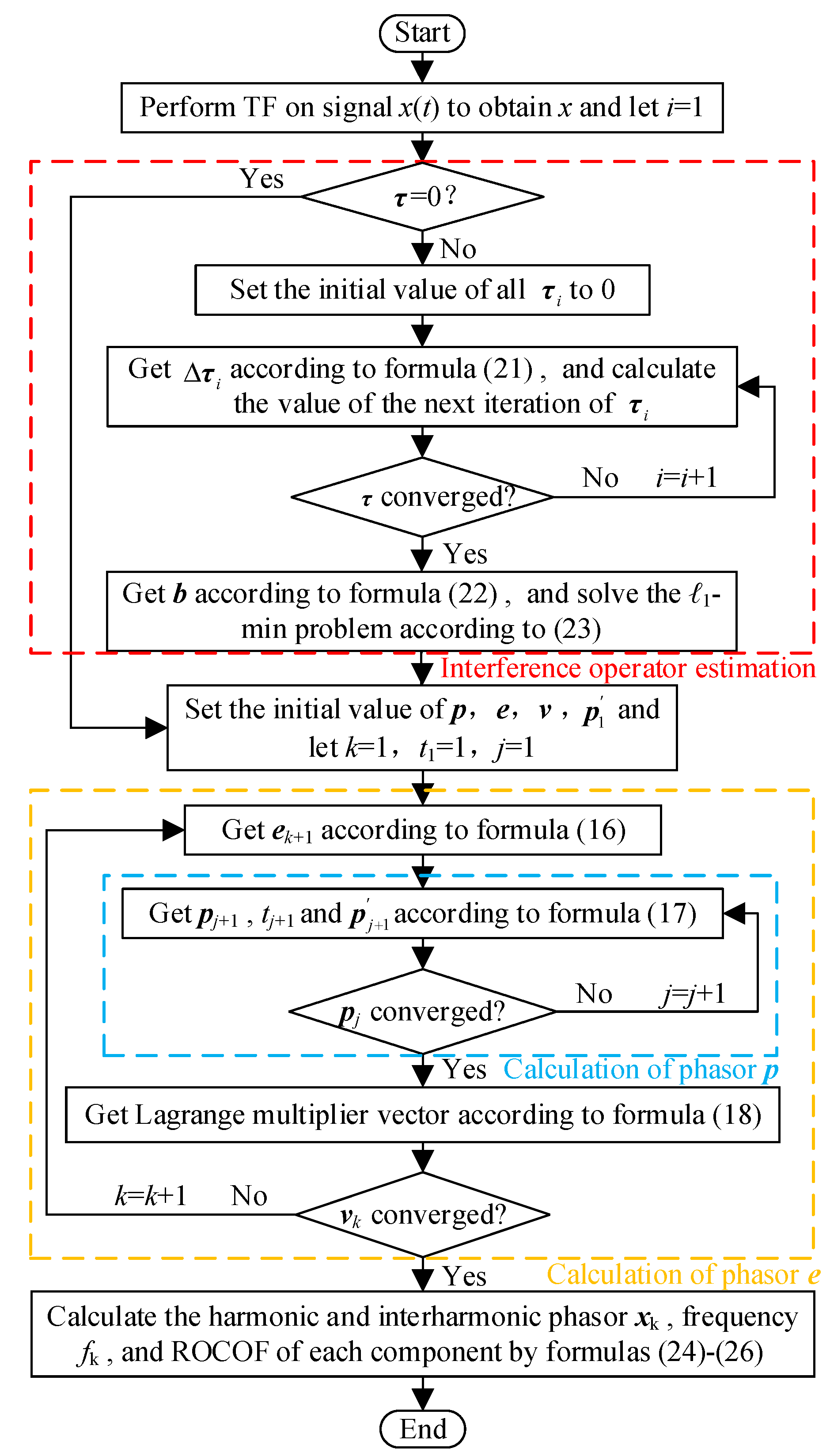
3. Fast Minimization Algorithm
3.1. ALM Method
3.2. Dynamic Change of the Amplitude and Frequenvy
4. Simulation Analysis
4.1. Basic Performance Test
4.2. Harmonic Modulation Test
4.3. Step Change Test
5. Conclusions
Author Contributions
Funding
Institutional Review Board Statement
Informed Consent Statement
Conflicts of Interest
Abbreviations
| WFDSs | Wide-frequency dense signals |
| FMA | Fast minimization algorithm |
| ALM | Augmented Lagrange multiplier |
| PMU | Phasor measurement unit |
| DFT | Discrete Fourier transform |
| RV-I | Rife–Vincent class I |
| ALLSSA | Antileakage least-squares spectral analysis |
| ALFT | Antileakage Fourier transform |
| MALLSSA | Multi-channel antileakage least-squares spectral analysis |
| SIFE | Sinc interpolation function-based estimator |
| HPE | Harmonic phasor estimator |
| DFSs | Dense frequency signals |
| PLL | Phase-locked loop |
| FLL | Frequency-locked loop |
| MWDFT | Moving-window discrete Fourier transform |
| FFT | Fast Fourier transform |
| TSCW | Triangular self-convolution window |
| MUSIC | Multiple signal classification |
| ESPRIT | Estimation of signal parameters via rotational invariance technique |
| MSSM | Multi-interharmonic spectrum separation and measurement |
| EMO | Exact model order |
| HHT | Hilbert–Huang transform |
| MMVs | Multiple measurement vectors |
| OMP | Orthogonal matching pursuit |
| CS | Compressive sensing |
| ADM | Alternation direction method |
| ROCOF | Rate of change of frequency |
| BPDN | Basis pursuit denoising |
| TVE | Total vector error |
| FE | Frequency error |
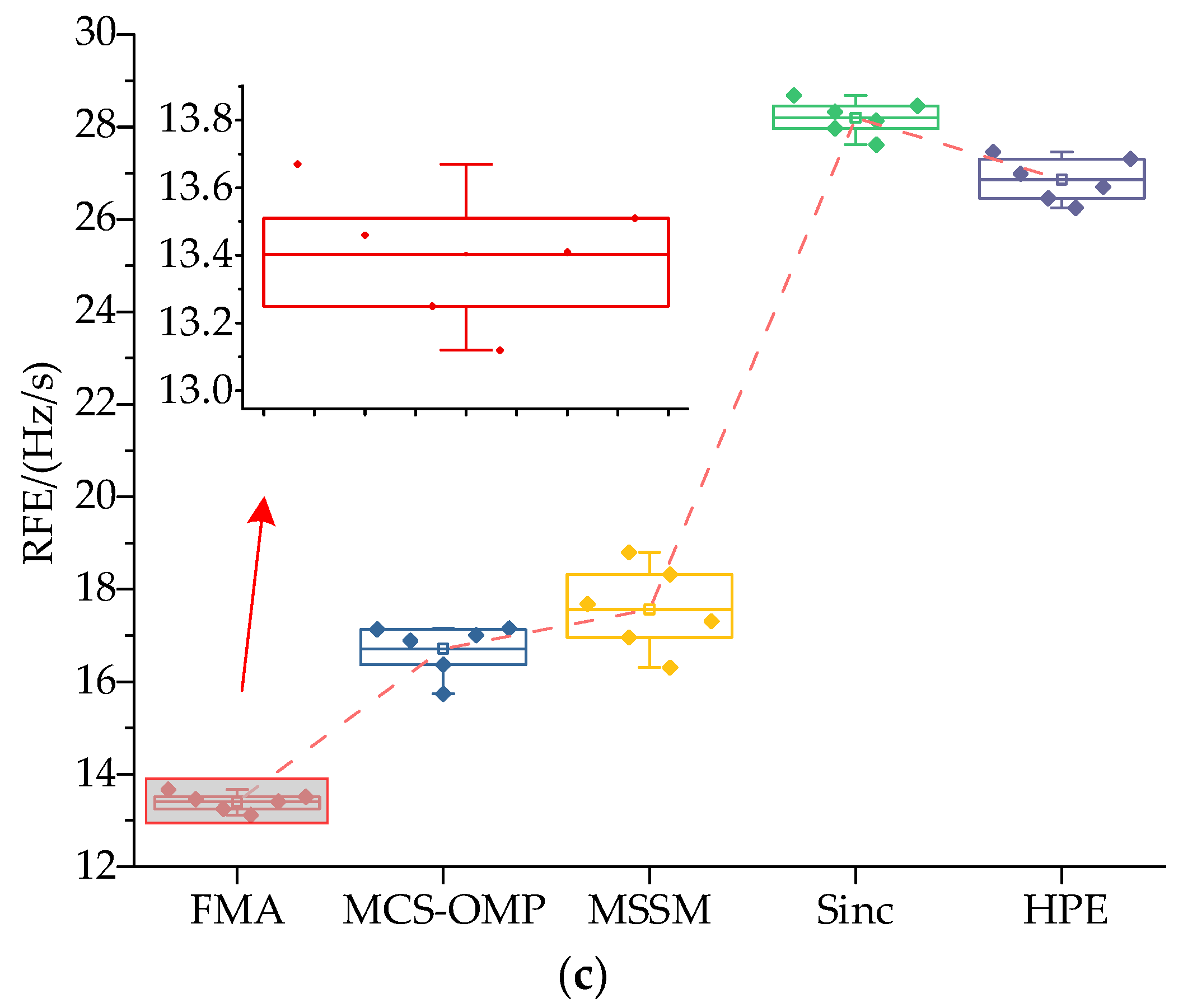
| RFE | Rate of change of frequency error |
References
- Ma, X.; Luo, H.; Yang, H. The Measurement and Analysis of Dense Frequency Signals Considering New Energy Integration. IEEE Trans. Power Deliv. 2021, 37, 3062–3070. [Google Scholar] [CrossRef]
- Kaczmarek, M.; Szczęsny, A.; Stano, E. Operation of the Electronic Current Transformer for Transformation of Distorted Current Higher Harmonics. Energies 2022, 15, 4368. [Google Scholar] [CrossRef]
- Chen, J.-H.; Tan, K.-H.; Lee, Y.-D. Intelligent Controlled DSTATCOM for Power Quality Enhancement. Energies 2022, 15, 4017. [Google Scholar] [CrossRef]
- Jafarpisheh, B.; Madani, S.M.; Jafarpisheh, S. Improved DFT-Based Phasor Estimation Algorithm Using Down-Sampling. IEEE Trans. Power Deliv. 2018, 33, 3242–3245. [Google Scholar] [CrossRef]
- Wang, K.; Wen, H.; Li, G. Accurate Frequency Estimation by Using Three-Point Interpolated Discrete Fourier Transform Based on Rectangular Window. IEEE Trans. Industr. Inform. 2021, 17, 73–81. [Google Scholar] [CrossRef]
- Lim, Y.C.; Saramäki, T.; Diniz, P.S.R.; Liu, Q. Fast Convergence Method for Scaling Window Sidelobe Magnitude. IEEE Signal Process. Lett. 2021, 28, 2078–2081. [Google Scholar] [CrossRef]
- Štremfelj, J.; Agrež, D. Nonparametric Estimation of Power Quantities in the Frequency Domain Using Rife-Vincent Windows. IEEE Trans. Instrum. Meas. 2013, 62, 2171–2184. [Google Scholar] [CrossRef]
- Ghaderpour, E.; Liao, W.; Lamoureux, M.P. Antileakage least-squares spectral analysis for seismic data regularization and random noise attenuation. Geophysics 2018, 3, V157–V170. [Google Scholar] [CrossRef]
- Xu, S.; Zhang, Y.; Pham, D.; Lambaré, G. Antileakage Fourier transform for seismic data regularization. Geophysics 2005, 70, V87–V95. [Google Scholar] [CrossRef]
- Ghaderpour, E. Multichannel antileakage least-squares spectral analysis for seismic data regularization beyond aliasing. Acta Geophys. 2019, 67, 1349–1363. [Google Scholar] [CrossRef]
- Chen, L.; Zhao, W.; Wang, Q.; Wang, F.; Huang, S. Dynamic Harmonic Synchrophasor Estimator Based on Sinc Interpolation Functions. IEEE Trans. Instrum. Meas. 2019, 68, 3054–3065. [Google Scholar] [CrossRef]
- Chen, L.; Zhao, W.; Xie, X.; Zhao, D.; Huang, S. Harmonic Phasor Estimation Based on Frequency-Domain Sampling Theorem. IEEE Trans. Instrum. Meas. 2021, 70, 1–10. [Google Scholar] [CrossRef]
- Golestan, S.; Guerrero, J.M.; Vasquez, J.C. Three-Phase PLLs: A Review of Recent Advances. IEEE Trans. Power Electron. 2017, 32, 1894–1907. [Google Scholar] [CrossRef] [Green Version]
- Singh, K.M.; Sumathi, P. Moving-Window DFT Based Frequency-Locked Loop for FM Demodulation. IEEE Commun. Lett. 2016, 20, 898–901. [Google Scholar] [CrossRef]
- Wen, H.; Zhang, J.; Meng, Z.; Guo, S.; Li, F.; Yang, Y. Harmonic Estimation Using Symmetrical Interpolation FFT Based on Triangular Self-Convolution Window. IEEE Trans. Ind. Inf. 2015, 11, 16–26. [Google Scholar] [CrossRef]
- Xu, S.; Liu, H.; Bi, T. A Novel Frequency Estimation Method Based on Complex Bandpass Filters for P-Class PMUs with Short Reporting Latency. IEEE Trans. Power Deliv. 2021, 36, 3318–3328. [Google Scholar] [CrossRef]
- Prasad, A.; Kundu, D.; Mitra, A. Sequential Estimation of the Sum of Sinusoidal Model Parameters. J. Stat. Plann. Inference 2008, 138, 1297–1313. [Google Scholar] [CrossRef] [Green Version]
- Jafarpisheh, B.; Madani, S.M.; Parvaresh, F.; Shahrtash, S.M. Power System Frequency Estimation Using Adaptive Accelerated MUSIC. IEEE Trans. Instrum. Meas. 2018, 67, 2592–2602. [Google Scholar] [CrossRef]
- Lewandowski, M.; Walczak, J. Current Spectrum Estimation Using Prony’s Estimator and Coherent Resampling. COMPEL Int. J. Comput. Math. Electr. Electron. Eng. 2014, 33, 989–997. [Google Scholar] [CrossRef]
- Drummond, Z.D.; Claytor, K.E.; Allee, D.R.; Hull, D.M. An Optimized Subspace-Based Approach to Synchrophasor Estimation. IEEE Trans. Instrum. Meas. 2021, 70, 1–13. [Google Scholar] [CrossRef]
- Sun, Z.; He, Z.; Zang, T.; Liu, Y. Multi-Interharmonic Spectrum Separation and Measurement Under Asynchronous Sampling Condition. IEEE Trans. Instrum. Meas. 2016, 65, 1902–1912. [Google Scholar] [CrossRef]
- Yalcin, N.A.; Vatansever, F. A New Hybrid Method for Signal Estimation Based on Haar Transform and Prony Analysis. IEEE Trans. Instrum. Meas. 2021, 70, 1–9. [Google Scholar] [CrossRef]
- Chang, G.W.; Chen, C.I. An Accurate Time-Domain Procedure for Harmonics and Interharmonics Detection. IEEE Trans. Power Delivery 2010, 25, 1787–1795. [Google Scholar] [CrossRef]
- Jain, S.K.; Singh, S.N. Exact Model Order ESPRIT Technique for Harmonics and Interharmonics Estimation. IEEE Trans. Instrum. Meas. 2012, 61, 1915–1923. [Google Scholar] [CrossRef]
- Sadinezhad, I.; Agelidis, V.G. Frequency Adaptive Least-Squares-Kalman Technique for Real-Time Voltage Envelope and Flicker Estimation. IEEE Trans. Ind. Electron. 2012, 59, 3330–3341. [Google Scholar] [CrossRef]
- Chen, C.I.; Chang, G.W.; Hong, R.C.; Li, H.M. Extended Real Model of Kalman Filter for Time-Varying Harmonics Estimation. IEEE Trans. Power Deliv. 2010, 25, 17–26. [Google Scholar] [CrossRef]
- Lin, H.C. Intelligent Neural Network-Based Fast Power System Harmonic Detection. IEEE Trans. Ind. Electron. 2007, 54, 43–52. [Google Scholar] [CrossRef]
- Laila, D.S.; Messina, A.R.; Pal, B.C. A Refined Hilbert-Huang Transform with Applications to Interarea Oscillation Monitoring. IEEE Trans. Power Syst. 2009, 24, 610–620. [Google Scholar] [CrossRef] [Green Version]
- Zhuang, S.; Zhao, W.; Wang, R.; Huang, S. New Measurement Algorithm for Supraharmonics Based on Multiple Measurement Vectors Model and Orthogonal Matching Pursuit. IEEE Trans. Instrum. Meas. 2019, 68, 1671–1679. [Google Scholar] [CrossRef]
- Frigo, G.; Giorgi, G.; Bertocco, M.; Narduzzi, C. Multifunction phasor analysis for distribution networks. In Proceedings of the 2016 IEEE International Workshop on Applied Measurements for Power Systems (AMPS), Aachen, Germany, 28–30 September 2016. [Google Scholar]
- Liu, W.; Jiang, Y.; Xu, Y. A Super Fast Algorithm for Estimating Sample Entropy. Entropy 2022, 24, 524. [Google Scholar] [CrossRef] [PubMed]
- Bertsekas, D.P. Nonlinear Programming, 2nd ed.; Athena Scientific: Belmont, MA, USA, 1999; pp. 3–37. [Google Scholar]
- Yang, J.; Zhang, Y. Alternation Direction Algorithms for l1-Problems in Compressive Sensing; Methods and Algorithms for Scientific Computing: Berkeley, CA, USA, 2009; pp. 250–278. [Google Scholar]
- Asif, M.S.; Romberg, J. Sparse Recovery of Streaming Signals Using l1-Homotopy. IEEE Trans. Signal Process. 2014, 62, 4209–4223. [Google Scholar] [CrossRef]
- IEEE Std C37.118.1a-2014 (Amendment to IEEE Std C37.118.1-2011); IEEE Standard for Synchrophasor Measurements for Power Systems—Amendment 1: Modification of Selected Performance Requirements. IEEE Power & Energy Society: New York, NY, USA, 2014; pp. 1–25.


| k | 1 | 2 | 3 | 4 | 5 | 6 | 7 | 8 | 9 | 10 | 11 |
|---|---|---|---|---|---|---|---|---|---|---|---|
| (Hz) | 50 | 100 | 150 | 51 | 98 | 3550 | 3700 | 3850 | 4050 | 4150 | 4300 |
| (%) | 100 | 1.60 | 5.00 | 3.00 | 1.20 | 0.20 | 0.15 | 0.34 | 0.12 | 0.24 | 0.25 |
| (rad) | 0.32 | 0.53 | 0.22 | 0.34 | 0.45 | 0.40 | 0.23 | 0.14 | 0.50 | 0.34 | 0.63 |
Publisher’s Note: MDPI stays neutral with regard to jurisdictional claims in published maps and institutional affiliations. |
© 2022 by the authors. Licensee MDPI, Basel, Switzerland. This article is an open access article distributed under the terms and conditions of the Creative Commons Attribution (CC BY) license (https://creativecommons.org/licenses/by/4.0/).
Share and Cite
Yuan, Z.; Liao, Z.; Tu, H.; Tu, Y.; Li, W. Analysis of Wide-Frequency Dense Signals Based on Fast Minimization Algorithm. Energies 2022, 15, 5618. https://doi.org/10.3390/en15155618
Yuan Z, Liao Z, Tu H, Tu Y, Li W. Analysis of Wide-Frequency Dense Signals Based on Fast Minimization Algorithm. Energies. 2022; 15(15):5618. https://doi.org/10.3390/en15155618
Chicago/Turabian StyleYuan, Zehui, Zheng Liao, Haiyan Tu, Yuxin Tu, and Wei Li. 2022. "Analysis of Wide-Frequency Dense Signals Based on Fast Minimization Algorithm" Energies 15, no. 15: 5618. https://doi.org/10.3390/en15155618
APA StyleYuan, Z., Liao, Z., Tu, H., Tu, Y., & Li, W. (2022). Analysis of Wide-Frequency Dense Signals Based on Fast Minimization Algorithm. Energies, 15(15), 5618. https://doi.org/10.3390/en15155618