
Numerical Assessments of Flow and Advective Transport Uncertainty for Performance Measures of Radioactive Waste Geological Disposal in Fractured Rocks


Abstract
:
1. Introduction
2. Materials and Methods
2.1. Mathematical Formulations
2.1.1. Conservation and State Laws
2.1.2. Fracture Generation
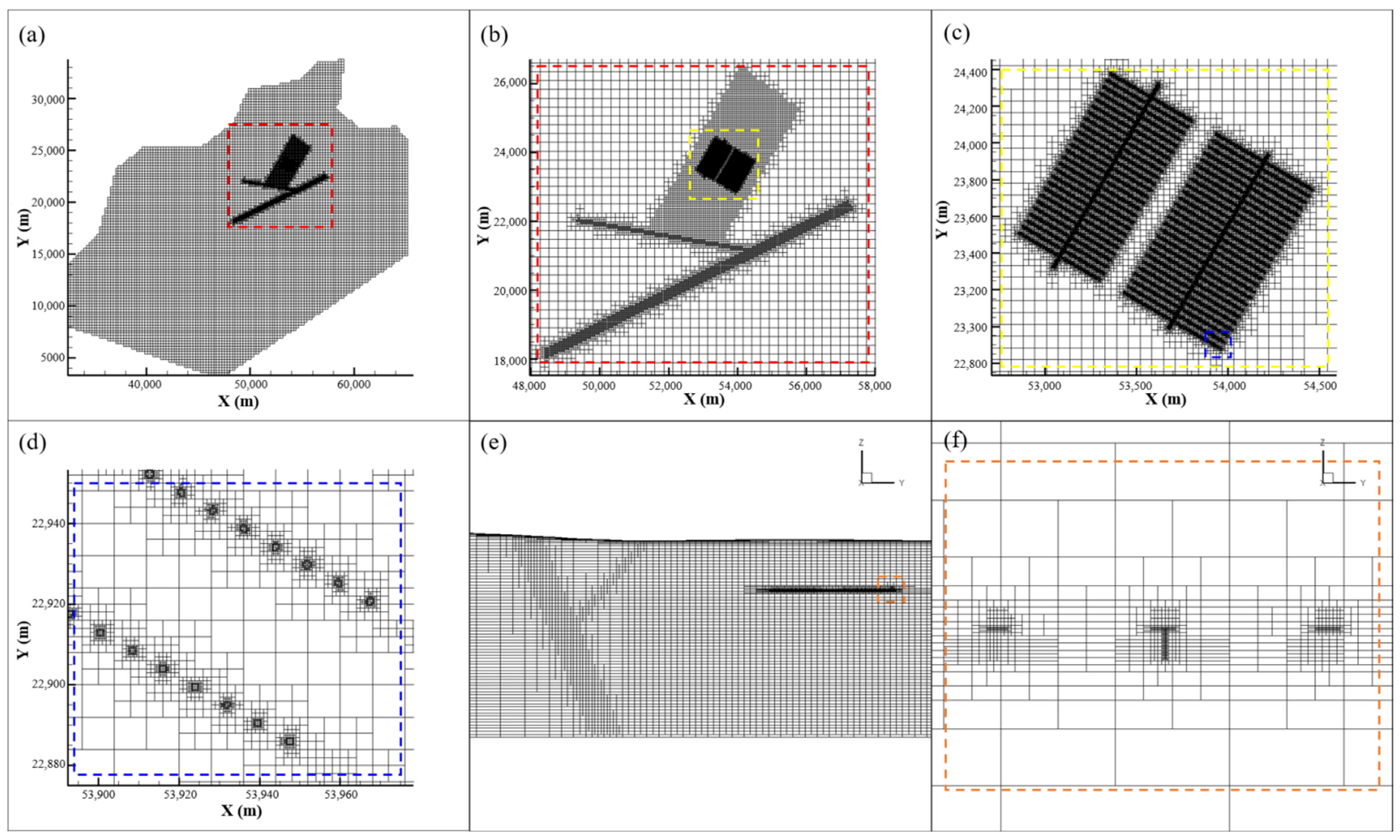
2.1.3. Computational Grids and Representation of Fractures on a Grid
2.1.4. Particle Tracking Algorithms
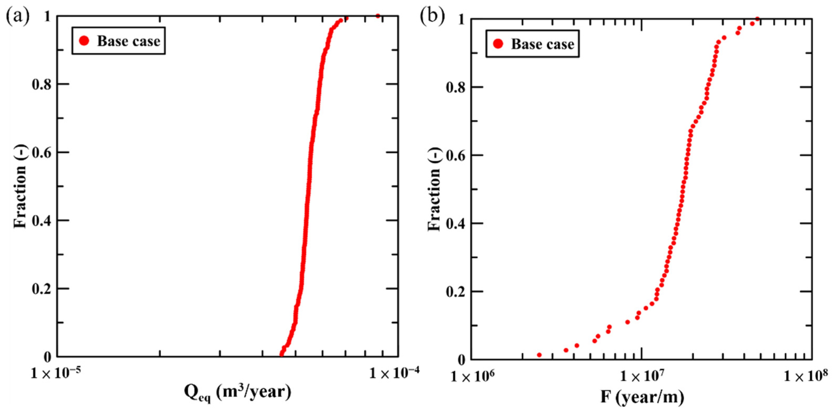
2.1.5. Performance Measures
2.2. Reference Case
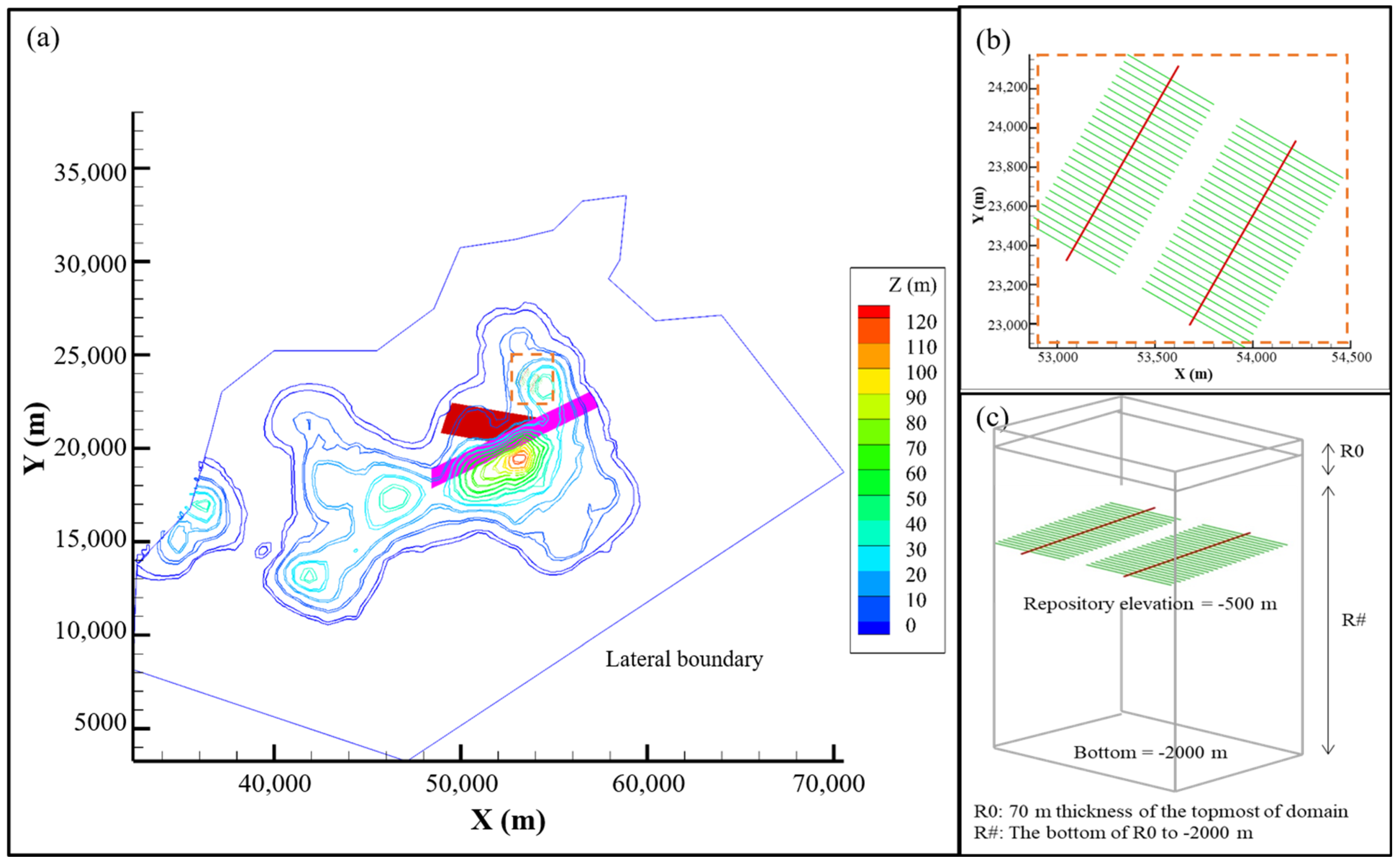
2.2.1. Conceptual Disposal Facility
2.2.2. Hydrogeological Conceptual Model

| Units | Lithology or Material | Distributions/Attitude and Width | Range of Hydraulic Conductivity (m/s) | Recommended Hydraulic Conductivity (m/s) | Porosity (-) |
|---|---|---|---|---|---|
| R0 | Regolith | 70 m thickness of the topmost domain | 5.0 × 10⁻⁶–1.0 × 10⁻⁴ | 1.0 × 10⁻⁵ | 1.0 × 10⁻³ |
| R# | Granitic gneiss | - | 4.1 × 10⁻¹²–1.0 × 10⁻⁹ | 1.0 × 10⁻¹⁰ | 5.4 × 10⁻³ |
| F1 | Fault | N64E/70N, 200 m width | 3.0 × 10⁻⁸–1.0 × 10⁻⁴ | 5.0 × 10⁻⁶ | 1.0 × 10⁻² |
| F2 | Fracture zone | N80E/50S, 20 m width | 3.0 × 10⁻⁸–1.0 × 10⁻⁴ | 5.0 × 10⁻⁶ | 1.5 × 10⁻² |
| MT | Backfill material | - | - | 1.0 × 10⁻¹⁰ | 4.0 × 10⁻¹ |
| DT | Backfill material | - | - | 1.0 × 10⁻¹⁰ | 4.0 × 10⁻¹ |
| DH | Buffer material | - | - | 1.0 × 10⁻¹² | 4.0 × 10⁻¹ |
| EDZ | Granitic gneiss | - | 3.3 × 10⁻⁹–3.3 × 10⁻⁷ | 3.3 × 10⁻⁸ * | 1.0 × 10⁻⁴ |
| Fracture Domain | R0 | R# | |
|---|---|---|---|
| Elevation | Depth below surface < 70 m | Depth below surface > 70 m | |
| Fracture clusters (Pole trend, pole plunge, κ, P32, rel) | Cluster 1 | (198, 18, 18, 26%) | (65, 17, 20, 15%) |
| Cluster 2 | (155, 4, 15, 24%) | (344, 38, 18, 24%) | |
| Cluster 3 | (264, 23, 16, 18%) | (281, 29, 16, 30%) | |
| Cluster 4 | (98, 81, 11, 32%) | (174, 22, 17, 10%) | |
| Cluster 5 | - | (175, 75, 19, 21%) | |
| Fracture intensity(P32) | 2.4 | 0.3 | |
| Fracture size | , | ||
| Fracture location | Stationary random (Poisson) process | Stationary random (Poisson) process | |
| Fracture transmissivity (T, m2⁄s) | T = 1.51 × 10 −7 × (L0.7); is the equivalent size (m) of a square fracture. | ; is the equivalent size (m) of a square fracture. | |
| Fracture Aperture (e, m) | |||
3. Numerical Examples
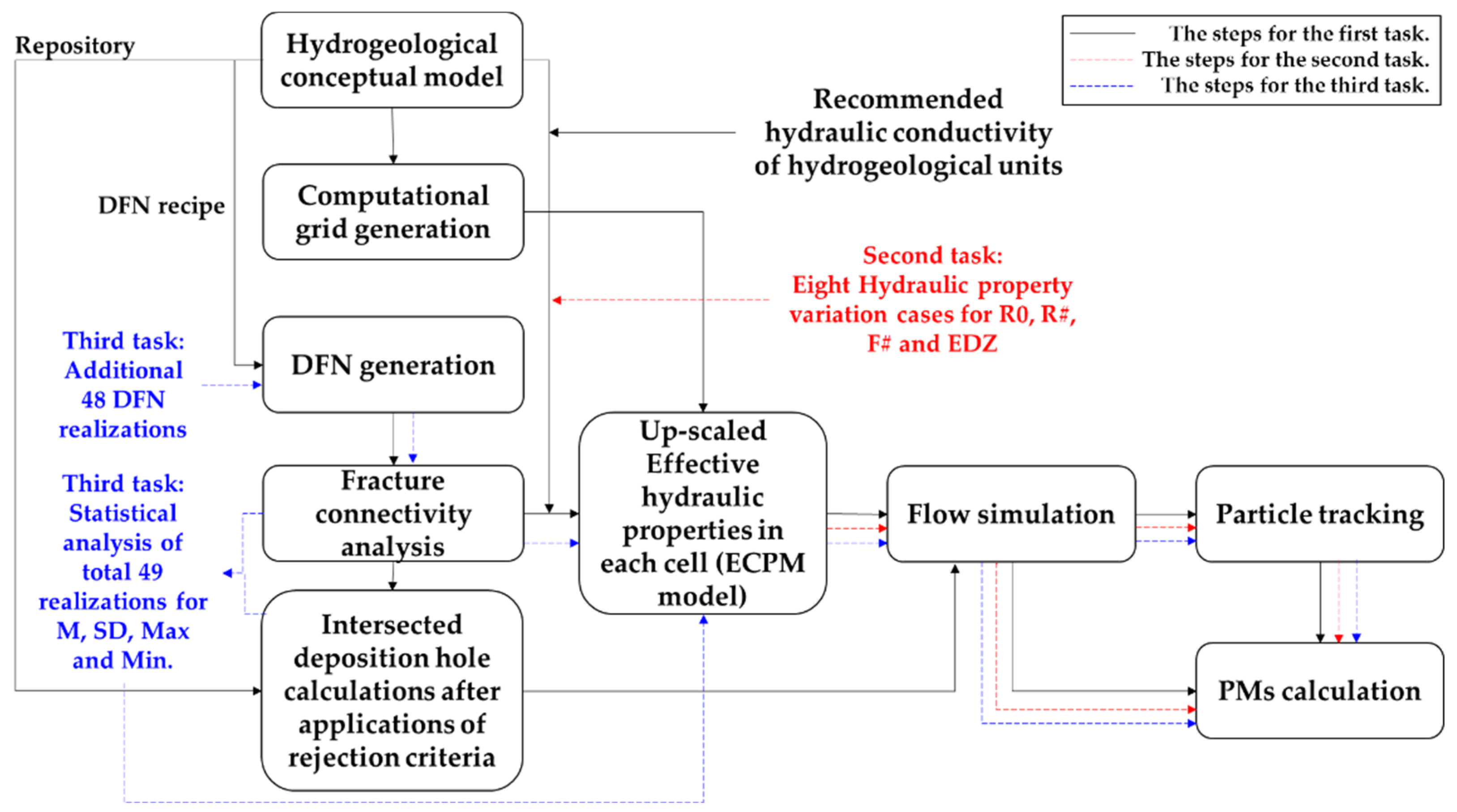
3.1. Workflow for the Study
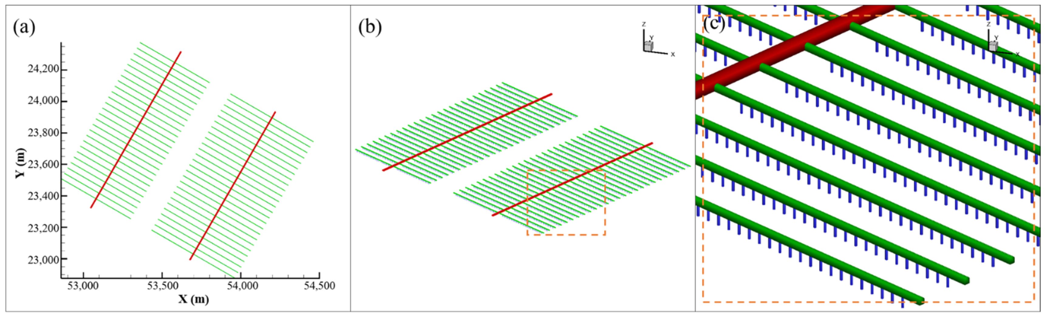
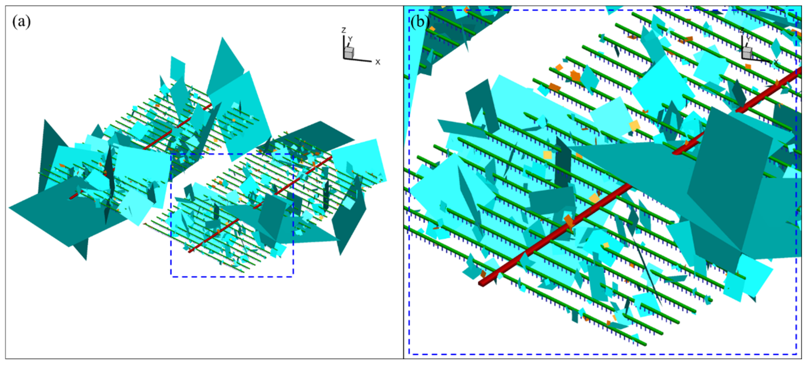
3.2. DFN Generation, Fracture Connectivity Analysis, and Intersections between Fractures and Repository
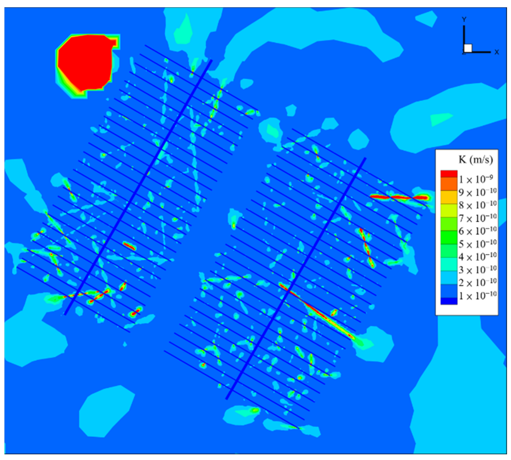
3.3. The Computational Grid and Effective Flow Properties Field for the Base Case
4. Results and Discussions
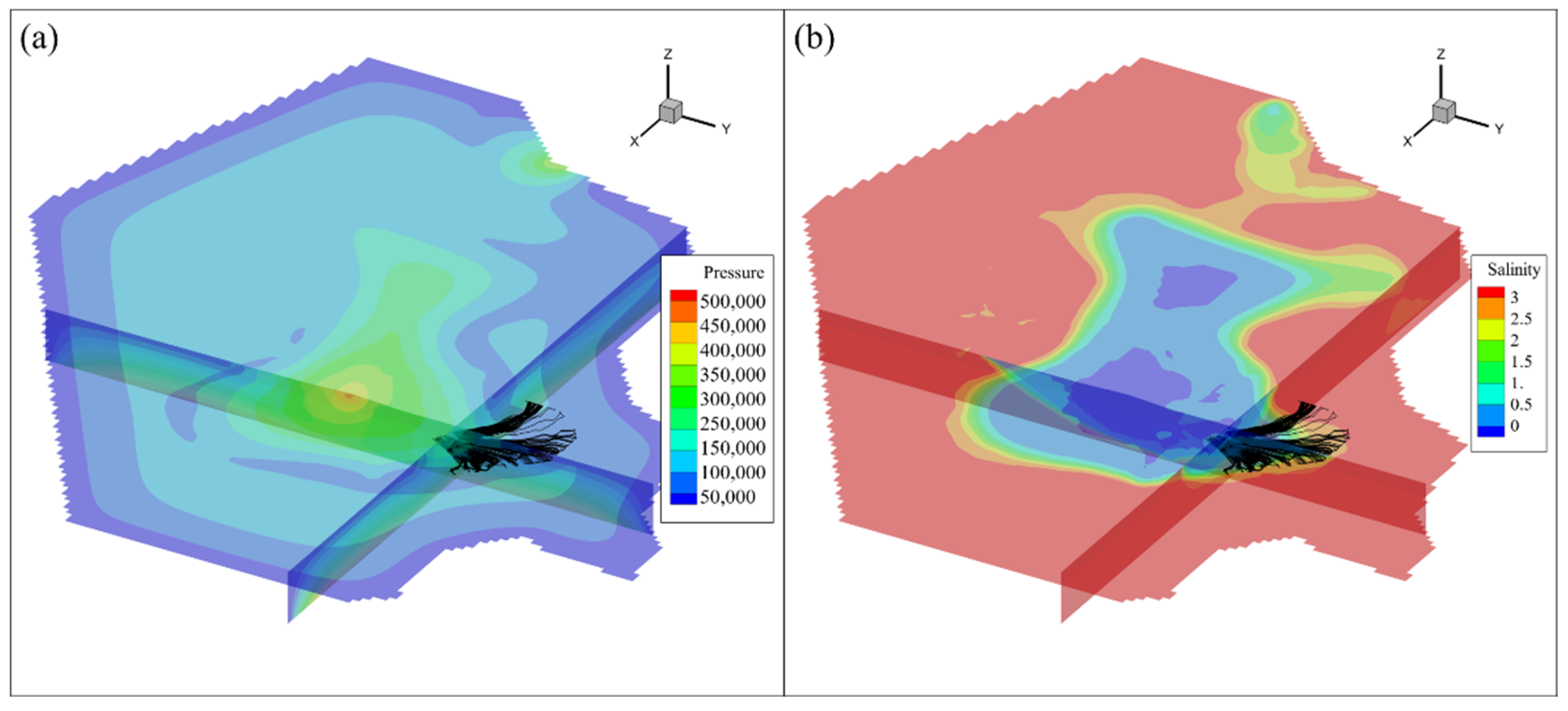
4.1. Steady-State Flow, Particle Tracking, and Calculation of PMs for the Base Case
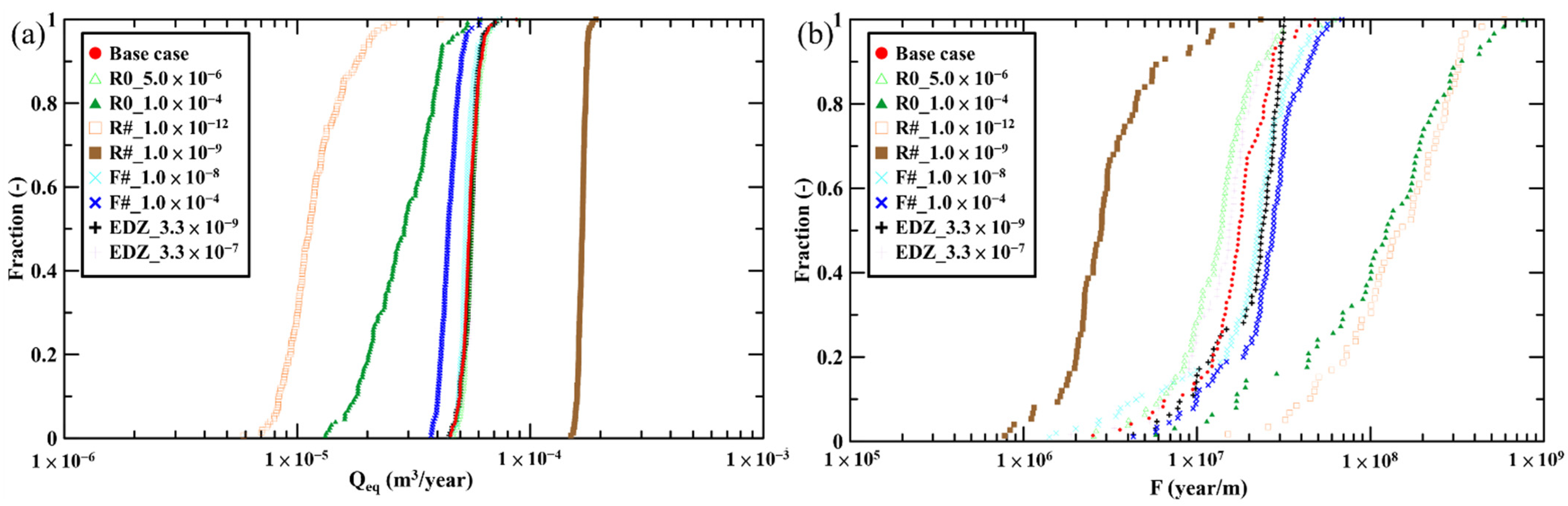
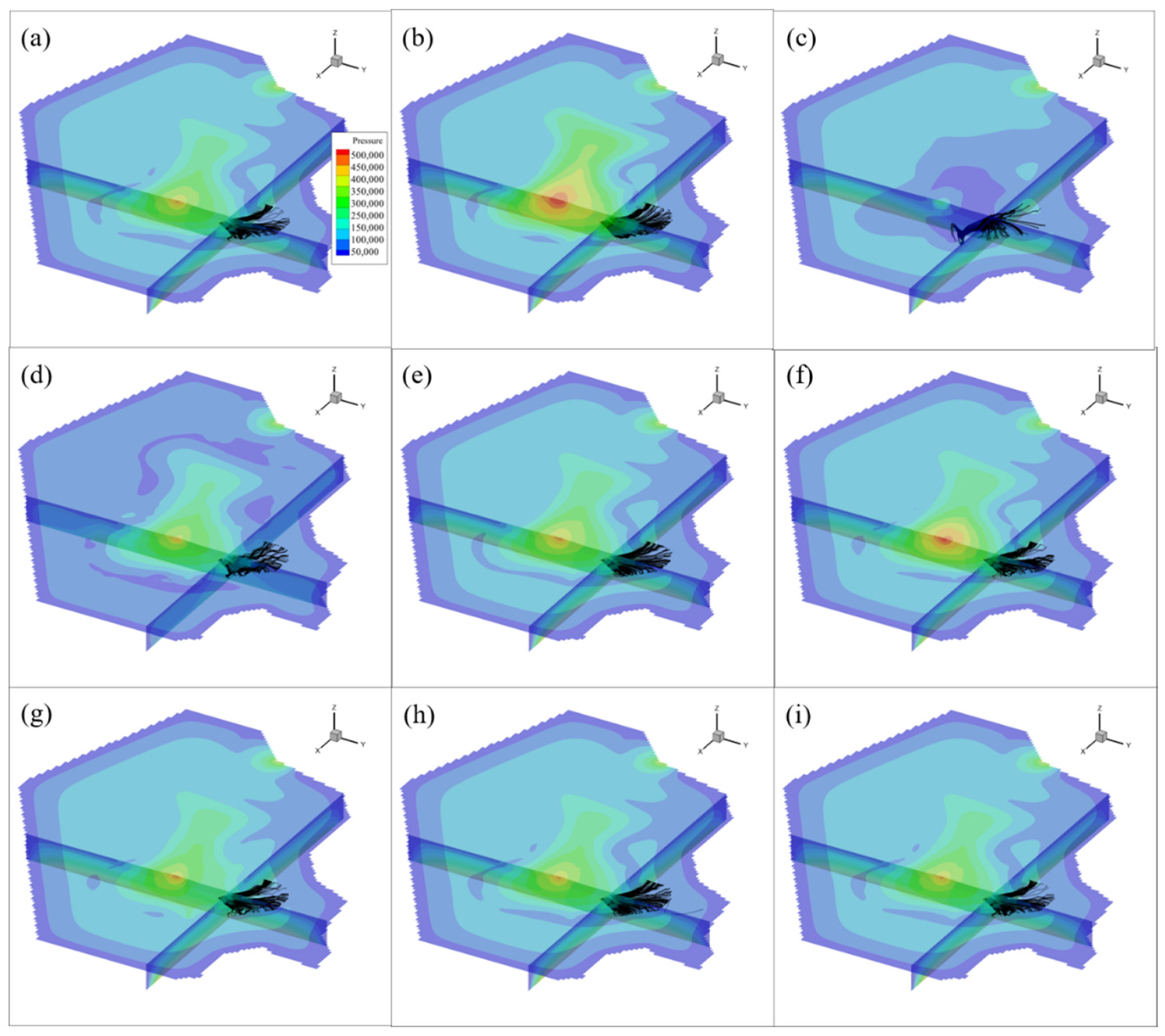
4.2. Sensitivity of Hydrogeological Units and EDZ on Flow, Particle Tracking, and PMs
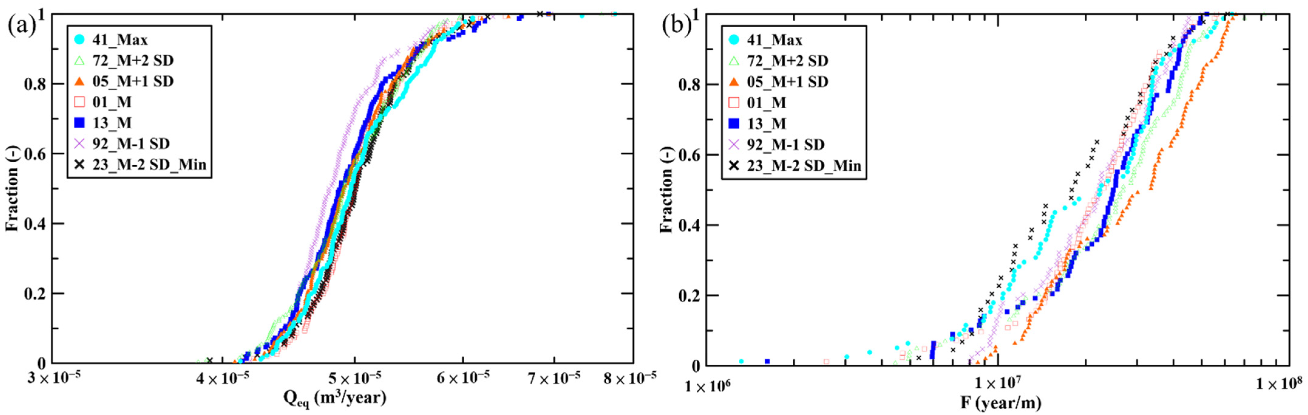
4.3. The Stochastic Simulations for 49 DFN Realizations
4.3.1. Effective Fracture Number
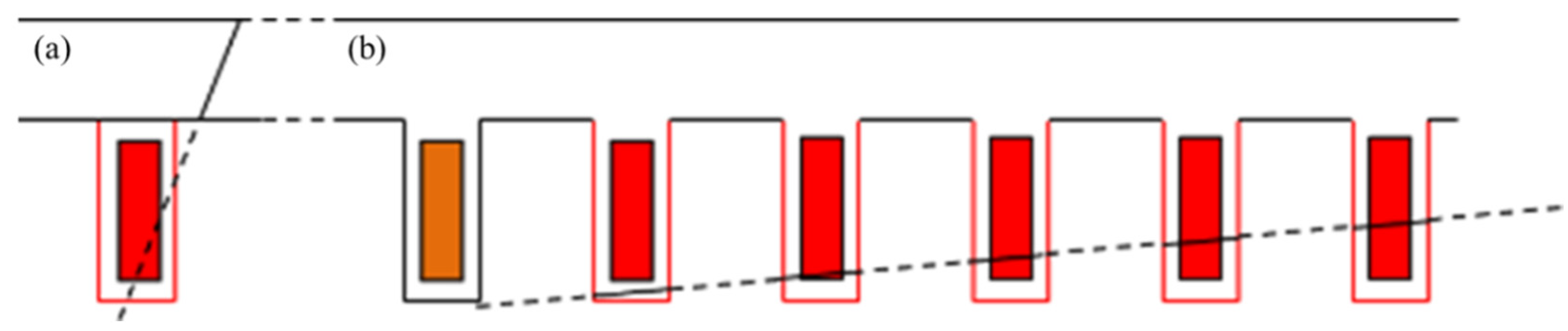
4.3.2. Remaining DHs Based on Rejection Criteria for the Q1 Path
5. Conclusions
Author Contributions
Funding
Institutional Review Board Statement
Informed Consent Statement
Data Availability Statement
Conflicts of Interest
References
- Hyman, J.D.; Gable, C.W.; Painter, S.L.; Makedonska, N. Conforming delaunay triangulation of stochastically generated three dimensional discrete fracture networks: A feature rejection algorithm for meshing strategy. J. Sci. Comput. 2014, 36, A1871–A1894. [Google Scholar] [CrossRef]
- Hyman, J.D.; Karra, S.; Makedonska, N.; Gable, C.W.; Painter, S.L.; Viswanathan, H.S. dfnWorks: A discrete fracture network framework for modeling subsurface flow and transport. Comput. Geosci. 2015, 84, 10–19. [Google Scholar] [CrossRef] [Green Version]
- Kalbacher, T.; Wang, W.; McDermott, C.; Kolditz, O.; Taniguchi, T. Development and application of a CAD interface for fractured rock. Eng. Geol. 2005, 47, 1017–1027. [Google Scholar] [CrossRef]
- Makedonska, N.; Painter, S.; Bui, Q.; Gable, C.; Karra, S. Particle tracking approach for transport in three-dimensional discrete fracture networks. Comput. Geosci. 2015, 19, 1123–1137. [Google Scholar] [CrossRef]
- Zhang, Q.H. Finite element generation of arbitrary 3-D fracture networks for flow analysis in complicated discrete fracture networks. J. Hydrol. 2015, 529, 890–908. [Google Scholar] [CrossRef]
- Chen, R.H.; Lee, C.H.; Chen, C.S. Evaluation of transport of radioactive contaminant in fractured rock. Environ. Geol. 2001, 41, 440–450. [Google Scholar] [CrossRef]
- Jing, L. A review of techniques, advances and outstanding issues in numerical modelling for rock mechanics and rock engineering. Int. J. Min. Reclam. Environ. 2003, 40, 283–353. [Google Scholar] [CrossRef]
- Rutqvist, J.; Leung, C.; Hoch, A.; Wang, Y.; Wang, Z. Linked multicontinuum and crack tensor approach for modeling of coupled geomechanics, fluid flow and transport in fractured rock. J. Rock Mech. Geotech. Eng. 2013, 5, 18–31. [Google Scholar] [CrossRef] [Green Version]
- Svensson, U.; Follin, S. Groundwater Flow Modelling of Excavation and Operational Phase—Forsmark; R-09-19; Svensk Kärnbränslehantering AB: Stockholm, Sweden, 2010. [Google Scholar]
- Vidstrand, P.; Follin, S.; Zugec, N. Groundwater Flow Modelling of Periods with Periglacial and Glacial Climate Conditions—Forsmark; R-09-21; Svensk Kärnbränslehantering AB: Stockholm, Sweden, 2010. [Google Scholar]
- Selroos, J.-O.; Follin, S. SR-Site Groundwater flow Modelling Methodology, Setup and Results; R-09-22; Svensk Kärnbränslehantering AB: Stockholm, Sweden, 2010. [Google Scholar]
- Nuclear Materials and Radioactive Waste Management Act. Available online: https://erss.aec.gov.tw/law/EngLawContent.aspx?lan=E&id=6 (accessed on 30 June 2022).
- Enforcement Rules for the Nuclear Materials and Radioactive Waste Management Act. Available online: https://law.moj.gov.tw/ENG/LawClass/LawAll.aspx?pcode=J0160034 (accessed on 19 July 2022).
- Taiwan Power Company. The Preliminary Technical Feasibility Study for Final Disposal of Spent Nuclear Fuel–2009 Progress Report (Summary); Taiwan Power Company: Taipei, Taiwan, 2009. [Google Scholar]
- Swedish Nuclear Fuel Supply Company. Final Storage of Spent Nuclear Fuel–KBS-3 (Summary); Swedish Nuclear Fuel Supply Company/Division KBS: Stockholm, Sweden, 1983.
- Taiwan Power Company. The Technical Feasibility Assessment Report on Spent Nuclear Fuel Final Disposal, Main Report; Potential Host Rock Characterization and Evaluation Stage; The Spent Nuclear Fuel Final Disposal Program; Taiwan Power Company: Taipei, Taiwan, 2017. [Google Scholar]
- Japan Nuclear Cycle Development Institute. H12: Project to Establish the Scientific and Technical Basis for HLW Disposal in Japan, Project Overview Report; Second Progress Report on Research and Development for the Geological Disposal of HLW in Japan; Japan Nuclear Cycle Development Institute: Tokyo, Japan, 2000. [Google Scholar]
- Svensk Kärnbränslehantering AB. Site Description of Forsmark at Completion of the Site Investigation Phase, SDM-Site Forsmark; TR-08-05; Svensk Kärnbränslehantering AB: Stockholm, Sweden, 2008. [Google Scholar]
- Joyce, S.; Simpson, T.; Hartley, L.; Applegate, D.; Hoek, J.; Jackson, P.; Swan, D. Groundwater Flow Modelling of Periods with Temperate Climate Conditions—Forsmark; R-09-20; Svensk Kärnbränslehantering AB: Stockholm, Sweden, 2010. [Google Scholar]
- Svensk Kärnbränslehantering AB. Long-Term Safety for the Final Repository for Spent Nuclear Fuel at Forsmark, Main Report of the DR-Site Project; TR-11-01; Svensk Kärnbränslehantering AB: Stockholm, Sweden, 2011. [Google Scholar]
- Svensk Kärnbränslehantering AB; POSIVA Oy. Safety Functions, Performance Targets and Technical Design Requirements for a KBS-3V Repository, Conclusion and Recommendations from a Joint SKB and Posiva Working Group; Posiva SKB Report, 01; Svensk Kärnbränslehantering AB: Stockholm, Sweden; POSIVA Oy: Eurajoki, Finland, 2017. [Google Scholar]
- Svensson, U. A continuum representation of fracture networks. Part I: Method and basic test cases. J. Hydrol. 2001, 250, 170–186. [Google Scholar] [CrossRef]
- Svensson, U. A continuum representation of fracture networks. Part II: Application to the Äspö Hard Rock laboratory. J. Hydrol. 2001, 250, 187–205. [Google Scholar] [CrossRef]
- Svensson, U.; Ferry, M. DarcyTools: A computer code for hydrogeological analysis of nuclear waste repositories in fractured rock. J. Appl. Math. Phys. 2014, 2, 365–383. [Google Scholar] [CrossRef]
- Svensson, U.; Kuylenstierna, H.-O.; Ferry, M. DarcyTools Version 3.4–Concepts, Methods and Equations; R-07-38; Svensk Kärnbränslehantering AB: Stockholm, Sweden, 2010. [Google Scholar]
- Svensson, U. DarcyTools Version 3.4–Verification, Validation and Demonstration; R-10-71; Svensk Kärnbränslehantering AB: Stockholm, Sweden, 2010. [Google Scholar]
- Svensson, U.; Ferry, M. DarcyTools Version 3.4–User’s Guide; R-10-72; Svensk Kärnbränslehantering AB: Stockholm, Sweden, 2010. [Google Scholar]
- Moreno, L.; Gylling, B. Equivalent Flow Rate Concept Used in Near Field Transport Model COMP23–Proposed Value for SR-97; R-98-53; Svensk Kärnbränslehantering AB: Stockholm, Sweden, 1998. [Google Scholar]
- Andersson, J.; Elert, M.; Gylling, B.; Moreno, L.; Selroos, J.-O. Derivation and Treatment of the Flow Wetted Surface and Other Geosphere Parameters in the Transport Models FARF31 and COMP23 for Use in Safety Assessment; R-98-60; Svensk Kärnbränslehantering AB: Stockholm, Sweden, 1998. [Google Scholar]
- Lee, T.P. Construction of DFN-Based Hydrogeological Model Using Reference Case Data for SNF Disposal in Taiwan. ARMA-DFNE-18-0820. In Proceedings of the 2nd International Discrete Fracture Network Engineering Conference, Seattle, WA, USA, 20 June 2018. [Google Scholar]
- Chiu, T.-H. The Application of Discrete Fracture Network Model for Taiwan SNF Final Disposal Program. ARMA-DFNE-18-0919. In Proceedings of the 2nd International Discrete Fracture Network Engineering Conference, Seattle, WA, USA, 20 June 2018. [Google Scholar]
- Liou, T.-S.; Huang, S.-Y.; Tien, N.-C.; Lin, W.; Lin, C.-K. Characterization of Groundwater Flow in a Fractured Crystalline Rock Mass Using Taiwan’s Reference Case Data. ARMA-DFNE-18-0285. In Proceedings of the 2nd International Discrete Fracture Network Engineering Conference, Seattle, WA, USA, 20 June 2018. [Google Scholar]
- Svensk Kärnbränslehantering AB. Buffer, Backfill and Closure Process Report for the Safety Assessment SR-Site; TR-10-47; Svensk Kärnbränslehantering AB: Stockholm, Sweden, 2010. [Google Scholar]
- Bäckblom, G. Excavation Damage and Disturbance in Crystalline Rock–Results from Experiments and Analyses; TR-08-08; Svensk Kärnbränslehantering AB: Stockholm, Sweden, 2008. [Google Scholar]


| Number of DH Intersected by Isolated Fractures | Number of DH Intersected by Connected Fractures | Number of DH with Rejection Criteria | Remained Number of DH for Q1 Path |
|---|---|---|---|
| 47 | 365 | 217 | 148 |
| Cases | Base Case | R0_5.0 × 10−6 | R0_1.0 × 10−4 | R#_1.0 × 10−12 | R#_1.0 × 10−9 | F#_1.0 × 10−8 | F#_1.0 × 10−4 | EDZ_3.3 × 10−9 | EDZ_3.3 × 10−7 |
|---|---|---|---|---|---|---|---|---|---|
| Maximum Qeq (m3/year) | 8.72 × 10⁻⁵ | 9.01 × 10⁻⁵ | 6.08 × 10⁻⁵ | 4.12 × 10⁻⁵ | 1.91 × 10⁻⁴ | 7.39 × 10⁻⁵ | 6.07 × 10⁻⁵ | 7.67 × 10⁻⁵ | 7.53 × 10⁻⁵ |
| Minimum Qeq (m3/year) | 4.55 × 10⁻⁵ | 4.69 × 10⁻⁵ | 1.32 × 10⁻⁵ | 5.88 × 10⁻⁶ | 1.49 × 10⁻⁴ | 4.55 × 10⁻⁵ | 3.76 × 10⁻⁵ | 4.62 × 10⁻⁵ | 4.48 × 10⁻⁵ |
| Maximum F (year/m) | 4.78 × 10⁷ | 6.15 × 10⁷ | 7.61 × 10⁸ | 5.91 × 10⁸ | 2.33 × 10⁷ | 6.17 × 10⁷ | 6.83 × 10⁷ | 5.33 × 10⁷ | 5.29 × 10⁷ |
| Minimum F (year/m) | 2.51 × 10⁶ | 2.54 × 10⁶ | 5.78 × 10⁶ | 1.51 × 10⁷ | 7.77 × 10⁵ | 1.41 × 10⁶ | 4.29 × 10⁶ | 2.24 × 10⁶ | 1.88 × 10⁶ |
| Realization number * | 01 | 02 | 03 | 04 | 05 | 06 | 07 | 08 | 09 |
| Fracture number ** | 8,320,632 | 8,341,248 | 8,156,556 | 8,278,347 | 8,285,150 | 8,300,106 | 8,239,884 | 8,225,342 | 8,252,640 |
| Realization number | 11 | 21 | 31 | 41 | 51 | 61 | 71 | 81 | 91 |
| Fracture number * | 8,195,941 | 8,253,067 | 8,237,262 | 8,265,553 | 8,385,158 | 8,264,897 | 8,301,048 | 8,241,552 | 8,230,608 |
| Realization number | 12 | 22 | 32 | 42 | 52 | 62 | 72 | 82 | 92 |
| Fracture number * | 8,273,013 | 8,231,334 | 8,253,960 | 8,279,343 | 8,308,163 | 8,206,153 | 8,269,453 | 8,219,716 | 8,210,454 |
| Realization number | 13 | 23 | 33 | 43 | 53 | 63 | 73 | 83 | 93 |
| Fracture number * | 8,235,503 | 8,353,253 | 8,258,874 | 8,214,399 | 8,304,313 | 8,186,264 | 8,205,598 | 8,238,796 | 8,295,528 |
| Realization number | 14 | 24 | 34 | 44 | 54 | 64 | 74 | 84 | 94 |
| Fracture number * | 8,246,436 | 8,204,342 | 8,267,200 | 8,245,352 | 8,247,883 | 8,243,216 | 8,273,206 | 8,241,587 | 8,228,915 |
| Realization number | 10 | 20 | 30 | 40 | - | - | - | - | - |
| Fracture number * | 8,182,334 | 8,269,977 | 8,191,695 | 8,283,339 | - | - | - | - | - |
| Parameters | Effective Fracture Number * | Realization Number |
|---|---|---|
| Min | 8,156,556 | 03 |
| Max | 8,385,158 | 51 |
| M | 8,253,971 | 32 |
| SD | 45,126 | - |
| M − 3 SD | 8,118,592 | - ** |
| M − 2 SD | 8,163,718 | 03 |
| M − 1 SD | 8,208,845 | 92 |
| M + 1 SD | 8,299,098 | 06 |
| M + 2 SD | 8,344,224 | 02 |
| M + 3 SD | 8,389,351 | 51 |
| Realization number * | 01 | 02 | 03 | 04 | 05 | 06 | 07 | 08 | 09 |
| Number of DH ** | 138 | 128 | 139 | 153 | 150 | 147 | 167 | 113 | 133 |
| Realization number | 11 | 21 | 31 | 41 | 51 | 61 | 71 | 81 | 91 |
| Number of DH | 132 | 141 | 152 | 168 | 142 | 142 | 143 | 153 | 114 |
| Realization number | 12 | 22 | 32 | 42 | 52 | 62 | 72 | 82 | 92 |
| Number of DH | 125 | 125 | 126 | 121 | 132 | 128 | 165 | 132 | 122 |
| Realization number | 13 | 23 | 33 | 43 | 53 | 63 | 73 | 83 | 93 |
| Number of DH | 138 | 112 | 133 | 130 | 140 | 146 | 130 | 148 | 139 |
| Realization number | 14 | 24 | 34 | 44 | 54 | 64 | 74 | 84 | 94 |
| Number of DH | 128 | 115 | 129 | 124 | 132 | 117 | 152 | 146 | 144 |
| Realization number | 10 | 20 | 30 | 40 | - | - | - | - | - |
| Number of DH | 148 | 142 | 149 | 126 | - | - | - | - | - |
| Parameters | Remaining Number of DH * | Realization |
|---|---|---|
| Min. | 112 | 23 |
| Max. | 168 | 41 |
| M | 137 | 1, 13 |
| SD | 14 | - |
| M − 3 SD | 96 | - ** |
| M − 2 SD | 109 | 23 |
| M − 1 SD | 123 | 92 |
| M + 1 SD | 150 | 5 |
| M + 2 SD | 164 | 72 |
| M + 3 SD | 178 | - ** |
Publisher’s Note: MDPI stays neutral with regard to jurisdictional claims in published maps and institutional affiliations. |
© 2022 by the authors. Licensee MDPI, Basel, Switzerland. This article is an open access article distributed under the terms and conditions of the Creative Commons Attribution (CC BY) license (https://creativecommons.org/licenses/by/4.0/).
Share and Cite
Yu, Y.-C.; Shen, Y.-H.; Lee, T.-P.; Ni, C.-F.; Lee, I.-H. Numerical Assessments of Flow and Advective Transport Uncertainty for Performance Measures of Radioactive Waste Geological Disposal in Fractured Rocks. Energies 2022, 15, 5585. https://doi.org/10.3390/en15155585
Yu Y-C, Shen Y-H, Lee T-P, Ni C-F, Lee I-H. Numerical Assessments of Flow and Advective Transport Uncertainty for Performance Measures of Radioactive Waste Geological Disposal in Fractured Rocks. Energies. 2022; 15(15):5585. https://doi.org/10.3390/en15155585
Chicago/Turabian StyleYu, Yun-Chen, Yu-Hsiang Shen, Tsai-Ping Lee, Chuen-Fa Ni, and I-Hsien Lee. 2022. "Numerical Assessments of Flow and Advective Transport Uncertainty for Performance Measures of Radioactive Waste Geological Disposal in Fractured Rocks" Energies 15, no. 15: 5585. https://doi.org/10.3390/en15155585
APA StyleYu, Y.-C., Shen, Y.-H., Lee, T.-P., Ni, C.-F., & Lee, I.-H. (2022). Numerical Assessments of Flow and Advective Transport Uncertainty for Performance Measures of Radioactive Waste Geological Disposal in Fractured Rocks. Energies, 15(15), 5585. https://doi.org/10.3390/en15155585