Medium-Term Forecasts of Load Profiles in Polish Power System including E-Mobility Development

Abstract

The main objective of this study was to conduct multi-stage and multi-variant prognostic research to assess the impact of e-mobility development on the Polish power system for the period 2022–2027. The research steps were as follows: forecast the number of electric vehicles (using seven methods), forecast annual power demand arising solely out of the operation of the forecast number of electric vehicles, forecast annual power demand with and without the impact of e-mobility growth (using six methods), forecast daily profiles of typical days with and without the impact of e-mobility growth (using three methods). For the purpose of this research, we developed a unique Growth Dynamics Model to forecast the number of electric vehicles in Poland. The application of Multi-Layer Perceptron (MLP) to the extrapolation of non-linear functions (to the forecast number of electric vehicles and forecast annual power demand without the impact of e-mobility growth) is our original, unique proposal to use the Artificial Neural Network (ANN). Another unique, innovative proposal is to include Artificial Neural Networks (Multi-Layer Perceptron and Long short-term memory (LSTM)) in an Ensemble Model for simultaneous extrapolation of 24 non-linear functions to forecast daily profiles of typical days without taking e-mobility into account. This research determined the impact of e-mobility development on the Polish power system, both in terms of annual growth of demand for power and within particular days (hourly distribution) for two typical days (summer and winter). Under the (most likely) balanced growth variant of annual demand for power, due to e-mobility, such demand would grow by more than 4%, and almost 7% under the optimistic variant. Percentage growth of power demand in terms of variation according to time of day was determined. For instance, for the balanced variant, the largest percentage share of e-mobility was in the evening “peak” time (about 6%), and the smallest percentage was in the night “valley” (about 2%).

1. Introduction

The last two decades have seen tremendous change in how electric power is used. On the one hand, certain users have reduced their demand for power. As a result of various regulations and technological progress, equipment (e.g., lighting, refrigerators, TV sets) has become increasingly energy efficient. On the other hand, growing population wealth has increased the quantities and diversities of power-consuming equipment (e.g., computers, air conditioners, heat pumps). In the Polish electric power system, a very characteristic symptom of these developments has been significantly increased demand for power in the summer months, especially during heat waves. At the same time, the hitherto typical winter peak of demand for electric power has been decreasing over the years. This requires changes to the planning of how the electric power system operates. Sufficient generation reserves and power transmission capacity should be ensured. To some extent, it leads to problems with upgrades and maintenance works in generation units and power transmission lines.

To operate the power system correctly, appropriate demand forecasts should be prepared, with various time horizons. Annual and monthly quantities of power are both important here, as are the aspects related to peak power and minimum power and the shape, or profile, of the demand curve. Power demand forecasts allow one to properly optimise the composition of the generating units and anticipated potential contingencies.

Electric vehicle owners are a new group of consumers that significantly affect the shape of the power demand curve. The research presented here aimed to answer the question as to the extent of the impact of electric vehicles on the demand profile of the Polish system in the medium term i.e., until 2027.

Over the period 2014–2021, the share of electric vans and cars in new vehicle sales in Poland rose from 0.04% to 2.86%. In that period, the number of EVs increased more than 80-fold [1]. The Polish Alternative Fuels Association forecasts that, by 2024, the market share (sales) of Battery Electric Vehicles (BEVs) will have increased by as much as 14 times, to 10% of the entire market for new vehicles in Poland. In 2025, the cumulative number of registered EVs (BEV and Plug-in Hybrid Electric Vehicles (PHEVs)) in Poland is forecast to be more than 516,000 vehicles, and more than 1.6 million by 2030 [1].

1.1. Related Works

In recent years, dynamic transition to electric vehicles (EVs) has become a major challenge facing the Green Transition. The predicted zero-emission future entails the need to anticipate the effects of progress in vehicle electrification. This involves a number of analyses, regarding both forecasts of the dynamics of development of EVs and their impact on the electric power system and its stability. The following five categories of studies on the topic have been identified in recent literature: forecasts of annual demand on the national level [2,3,4,5,6,7,8,9], forecast number of EVs [7,8,9,10], analyses of EV impacts on the power system [11,12], forecast power demand profiles [13,14,15,16,17,18,19], and studies combining these particular aspects [20,21,22,23,24,25,26].

The identified papers addressing annual demand applied to various parts of the world. Nayyar Hussain Mirjat et al. [2] used the Long-range Energy Alternatives Planning System (LEAP) model to analyse the effect of energy policies on Pakistan’s demand until 2050. Similar research using the same system, but for Ethiopia, was conducted by Gebremeskel, Ahlgren and Beyene [3]. The former compared four scenarios, including ones that address maximisation of energy efficiency, Renewable Energy Sources (RESs) penetration, or clean coal technologies. The latter determined scenarios depending on the level of economic development, electrification and urbanisation. Unlike the former, the latter provided for replacement of traditional cars with EVs, which was assumed to be achieved by 2050. Other research in this segment focused on traditional improvement of stability or quality of forecasts. Angelopoulos, Siskos and Psarras [4] proposed, for the Greek system, a disaggregation framework aimed at achieving a robust additive model. He, Wang, Guang and Zhao [5] presented the Simulated Annealing Chicken Swarm Optimization (SACWO) method to optimise the weights adopted in forecast models, and Manowska [6] presented the application of LSTM to power demand by user groups (residential, commercial, transport, industry, and agriculture).

Determination of annual national demand is used for finding a baseline for changes in energy demand as a result of progressing electrification of vehicle fleets. Another contribution of research on EV impacts is to determine the scale of this development by using certain assumptions [3,10] or forecasts [7,8,9]. This can be done in various ways. Wu & Chen [7] proposed Principal Component Analysis—General regression neural network (PCA-GRNN) as the prediction method. Rietmann, Hügler & Lieven [8] applied a logistic growth model, and Ding and Li [9] applied seven varied models, including ones based on the Grey Model. Some papers [7,8] addressed forecasts of the number of cars sold rather than the number of vehicles actually present in the market. Although such an approach allows for a clearer overview of the situation, based on economic factors, it fails to answer the question of how many cars there are on the market at the same time, which makes it necessary to adopt additional assumptions in longer forecast horizons. Unlike their predecessors, Viri, Makinen and Liimatainen [10] applied a scenario model to analyse the baseline and ±30% larger increase in the number of EVs. The baseline scenario was defined using a Suomen alueellinen autokantamalli, Finnish regional car fleet model (SALAMA). This model allowed for the inclusion of factors such as car age, age of car retirement, user’s age group, etc.

After the future number of vehicles is determined, the impact of that number of vehicles on the system can be defined. Such two-step analyses were conducted by Liu and Liu [20], Nogueira, Sousa and Alves [21], Wörner et al. [22], and Brdulak, Chaberek and Jagodziński [23]. The aspects addressed by them included analysis of the impact of vehicles on the peak and off-peak grid balance [21] and analysis of the sufficiency and development needs of charging infrastructure [22]. Other topics included the definition of changes in annual and monthly peak power [20] and the effect of Personal light electric vehicles (PLEVs), such as scooters, on the power grid load. However, the number of vehicles was not always necessary in EV impact studies. The paper by Galvin [11] attempted, instead, to determine how changes in specifications, such as weight and EV motor power output, affect consumption of energy. Feng et al. [12] focused on forecasts of load of vehicle charging stations.

The shape of future power demand profiles can be useful in determining the trends of change in relation to the traditional process of power delivery to users. It makes it possible to determine how the currently-used system balancing solutions might potentially evolve. In the literature considered here, research addressing forecast profiles of power demand has been quite diverse. Kalhori, Emami, Fallahi and Tabarzadi [13] presented a fuzzy logic system for demand with temperature uncertainty; Carmo, Souza and Barbosa [14] proposed a bottom-up approach to creating scenarios for daily curves based on demand, divided into Residential, Tertiary and Industry segments. A different approach was used in papers by Brodowski, Bielecki and Filocha [15] and Hinde, Verdejo and Martínez-Ramón [16], since they focused on creating a hybrid forecasting system. The former approach was based on using Principal Component Analysis (PCA) and clustering of data using Fuzzy C-Means to create a set of hierarchical demand estimators. The latter approach integrated regression and clustering. A secondary objective of the latter approach was to obtain feedback on how automatic division of demand into clusters has been achieved in hourly, daily and monthly intervals. The remaining identified papers also included analyses of the effect of COVID-19 on energy consumption and daily demand curve [17], standardisation of the modelling of load profiles for Europe [18] or forecasts of EV charging profiles [19]. The latter can also be found in Liu and Liu [20], with typical daily curves for subsequent years.

Some studies, classified as combining certain aspects, included the determination of the number and impact of EVs on the electric power system [20,21,22,23]. The remaining papers were more extensive, or featured slightly different characteristics. Piotrowski et al. [24] additionally analysed changes in daily profiles over the years. The research by Zou et al. [25] combined EV charging scenarios with effect on the sufficiency of charging infrastructure. Bibak and Tekiner-Mogulkoc [26] focused on EV control in various scenarios using Vehicle-to-grid (V2G) and its impact on daily profiles. The factors affecting the acceptance of that mechanism were presented by Heuveln et al. [27].

1.2. Objective and Contribution

The purpose of this paper was to conduct multi-stage and multi-variant prognostic studies (multiple secondary objectives) with the final objective being to determine the magnitude of impact of e-mobility on the Polish electric power system by 2027 (annual power demand figures). In addition, this paper determined the effect of e-mobility development on hourly profiles of power demand for typical winter and summer days. An important indirect objective was to develop methods to forecast the relative profiles for typical winter and summer days without taking into account the effect of e-mobility.

The research presented in this paper, compared to other studies on the impact of e-mobility on the Polish electric power system, is distinguished by the most comprehensive approach allowing the obtaining of more accurate results than studies using certain simplifications. These simplifications applied either to assumptions in relation to forecasts or the forecasts concerning only one research aspect (e.g., forecasts of annual electricity demand without the impact of e-mobility [6,28], forecasts of annual energy demand resulting from e-mobility [29]). As examples of the comprehensiveness of our presented approach, two elements can be mentioned. The first element is the division of the forecasted number of EVs into different categories of vehicles, thanks to which the estimation of energy demand is more accurate than in studies that do not take into account different EV categories. The second is the inclusion of the increase in the annual demand for electricity resulting from factors other than e-mobility in forecasting the shapes of daily profiles of typical days. It is worth adding that the proposed methodology of forecasting changes in the shape of daily profiles of typical days is a unique, innovative research. The most similar studies, but using simplified (linear) methods of forecasting of the shapes of typical days’ daily profiles, are described in [24]. The linear model is unable to represent the non-linear shape of the variability of power demand in the respective hour over consecutive years. Furthermore, to apply linear regression, one needs to build 24 independent models for the given typical day, whereas a single neural network (non-linear model) simultaneously generates 24 values of the typical day profile in a single step.

Below are listed the selected contributions of this paper:

• Application of the MLP artificial neural network for the extrapolation of non-linear function (forecast number of electric vehicles in Poland from 2022 to 2027), which is our original, unique proposal to apply ANN.
• Development of an original, unique Growth Dynamics Model, using forecasts of the ratio of annual growth rate to the forecast number of electric vehicles in Poland from 2022 to 2027.
• Application of the MLP artificial neural network for extrapolation of non-linear function (forecast annual power demand in Poland from 2022 to 2027, excluding the development of e-mobility in Poland), which is our original, unique proposal to use ANN.
• Application of combined artificial neural networks (MLP and LSTM) in an Ensemble Model for simultaneous extrapolation of 24 non-linear functions, which is our original, unique proposition to use ANN in forecasting the shapes of daily profiles of typical days for 2022–2027 without e-mobility.

The remainder of this paper is organised as follows: Section 2 presents the characteristics of the applied data time series. Section 3 specifies forecasting methods used in this paper and results of stepwise, multi-stage forecasts (Section 3.2 and Section 3.3), the final objectives of which are to forecast daily profiles of energy demand in the Polish electric power system, taking into account the development of e-mobility. Evaluation criteria used for the assessment of forecasting quality are presented in Section 3.1. Discussion is in Section 4. Finally, the main conclusions of our studies are summarised in Section 5, and references are listed at the end of this paper.

2. Data

Different time series from Poland were applied to multi-stage research which has as its primary end objective medium-term forecasts of the shape of daily profiles of power demand in the Polish electric power system, taking into account the development of e-mobility. The next research steps used a total of six different types of time series.

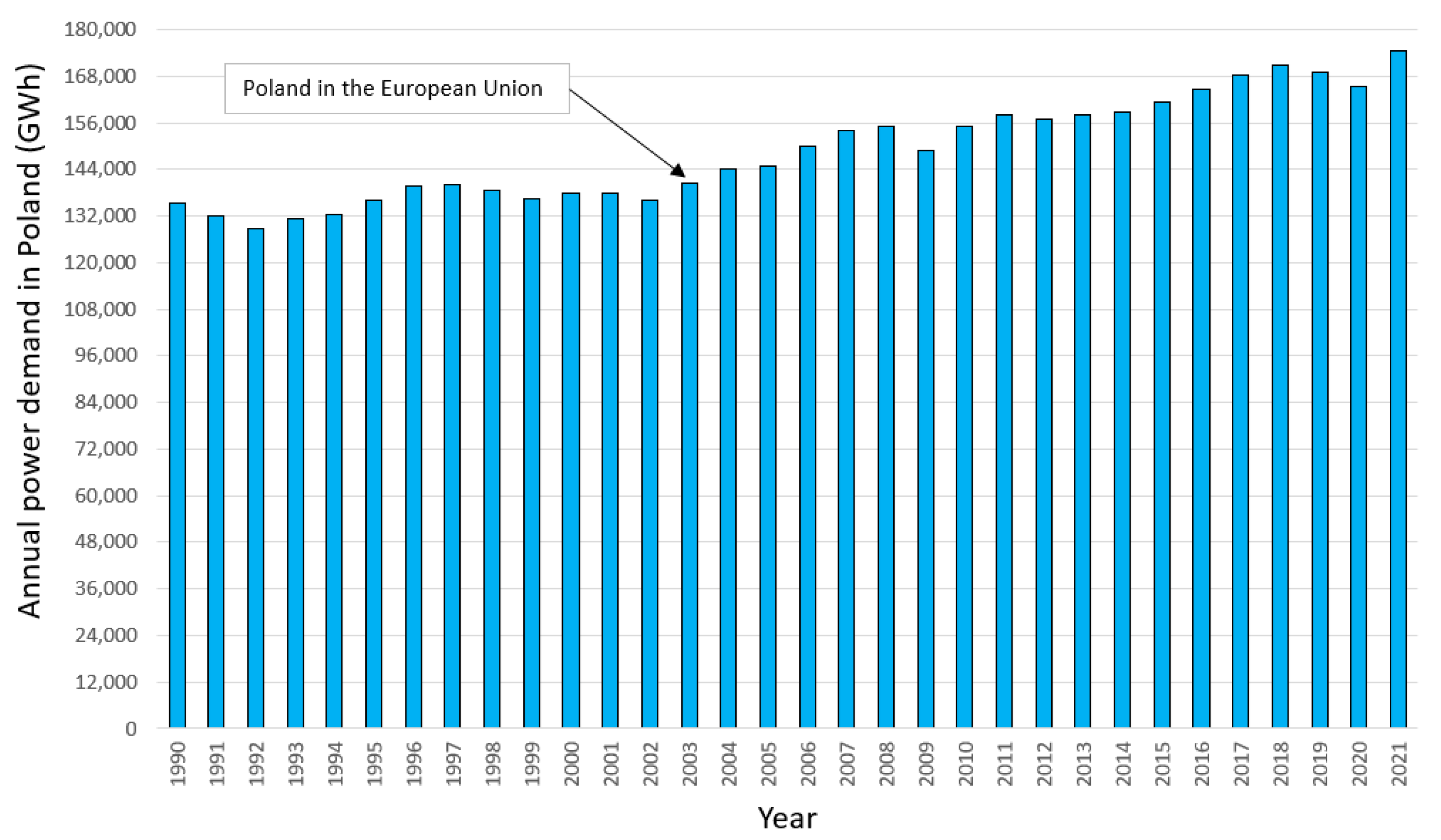
The first time series were annual values for electric power demand in Poland from 1990 to 2021 (a total of 32 values). The time series was used for forecasting annual values of power demand within a six years’ horizon (2022–2027). Figure 1 presents historical data for annual power demand. The process generally displayed a growing multi-annual trend, with temporary disturbances (drops in energy demand) due to economic situation (e.g., financial crisis 2007–2009, COVID-19 pandemic in 2019–2020). The growing trend was markedly more dynamic since Poland joined the European Union (EU) in 2004.

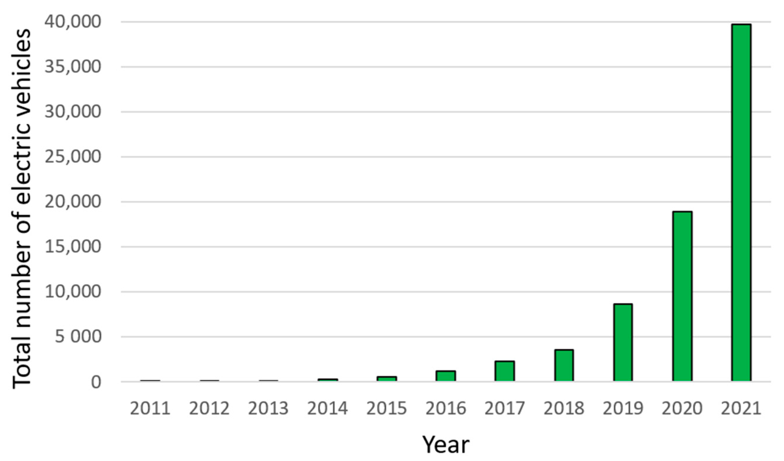
The second time series were cumulative values of the number of EVs in Poland since 2011 through to 2021 (a total of 11 values). The time series was used for forecasting the cumulative number of EVs in a six years’ horizon (2022–2027). Figure 2 presents the total number of EVs in Poland (2011–2021). The process involved strongly non-linear growth, particularly evident in the last three years.

The third type of time series were six-year forecasts (2022–2027) of power demand due to e-mobility development in Poland, in three variants (optimistic, balanced and pessimistic). The time series were calculated based on the forecast number of EVs in the six years’ horizon (2022–2027) and various EV statistical figures (including estimates of annual power demand per EV).

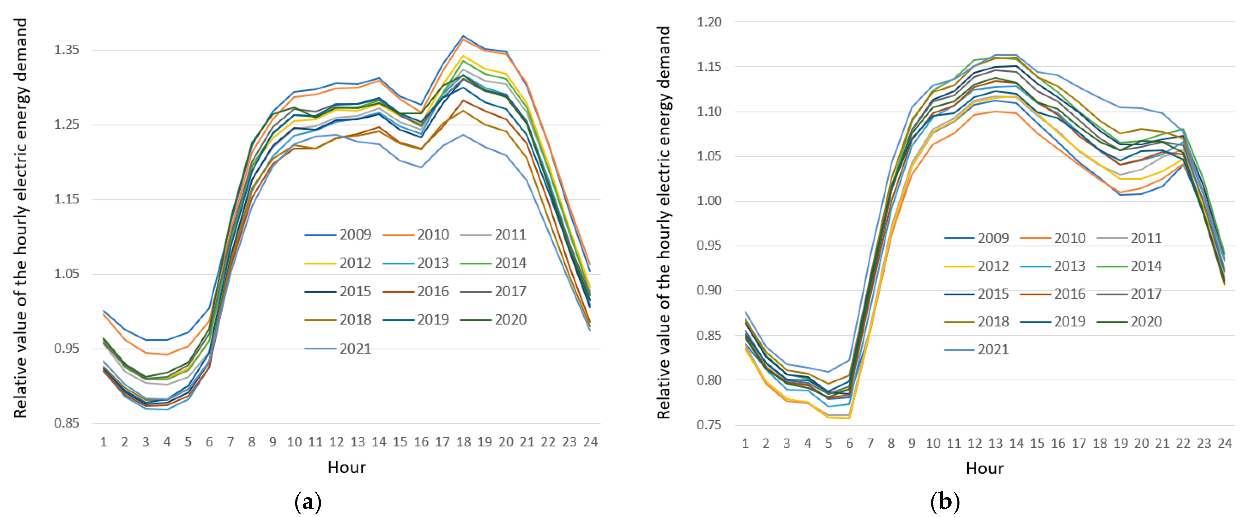
The fourth type of time series were hourly values of power demand in the national electric power system from 2009 to 2021 (a total of 13 years of hourly values). This time series was used to construct profiles of typical days for each of the 13 years. The third Wednesday of January and the third Wednesday of July are “typical days” in the Polish Power System, representing the winter and the summer business days, respectively [24]. Two daily profiles of typical days were calculated for each year of 2009–2021. The hourly values of the profile were computed as an arithmetic average of hourly values from five business Wednesdays. The five business Wednesdays were the following: the typical day (the third Wednesday of January or the third Wednesday of July), two prior business Wednesdays and two following business Wednesdays. This exercise evened out the profiles and reduced the random component resulting from single days.

Upon building the profiles of typical days for 13 years (2009–2021), two time series of the fifth type were established, containing 24 hourly values for the typical day profiles, for each of the 13 years. Hourly values of both profiles were normalised in each year separately. Normalisation was achieved by dividing the values of profiles from each hour by average hourly power demand during the year [24]. Normalisation enabled us to the track changes in the profiles in 2009–2021, ignoring any profile change resulting from multi-annual growing trends of power demand in the subsequent years. Figure 3 presents relative values of daily profiles of electric energy demand for the typical winter day and summer day in Poland from 2009 to 2021. The charts show that the profile of typical days changed over subsequent years. For the profile of the typical winter day, power demand was decreasing in subsequent years, albeit unevenly for particular hours. For the profile of the typical summer day, power demand has been growing unevenly. Based on these two time series, both profiles with six years’ horizons (2022–2027) were forecast, without taking into account an increase in power demand due to e-mobility development.

The sixth type of times series were daily profiles of power demand for various EV types (BEV, PHEV, electric buses, electric heavy trucks and electric delivery vans) and two different charging methods (slow charging and rapid charging). These profiles were expertly developed and uniquely based on different statistical data. The profiles were used for the final calculation of forecast profiles of typical days in the power system with the six years’ horizon (2022–2027), taking into account e-mobility development. In addition, this process required forecasts of annual EV numbers (2022–2027) and forecasts of annual power demand without taking into account e-mobility development (2022–2027).

3. Methods and Results

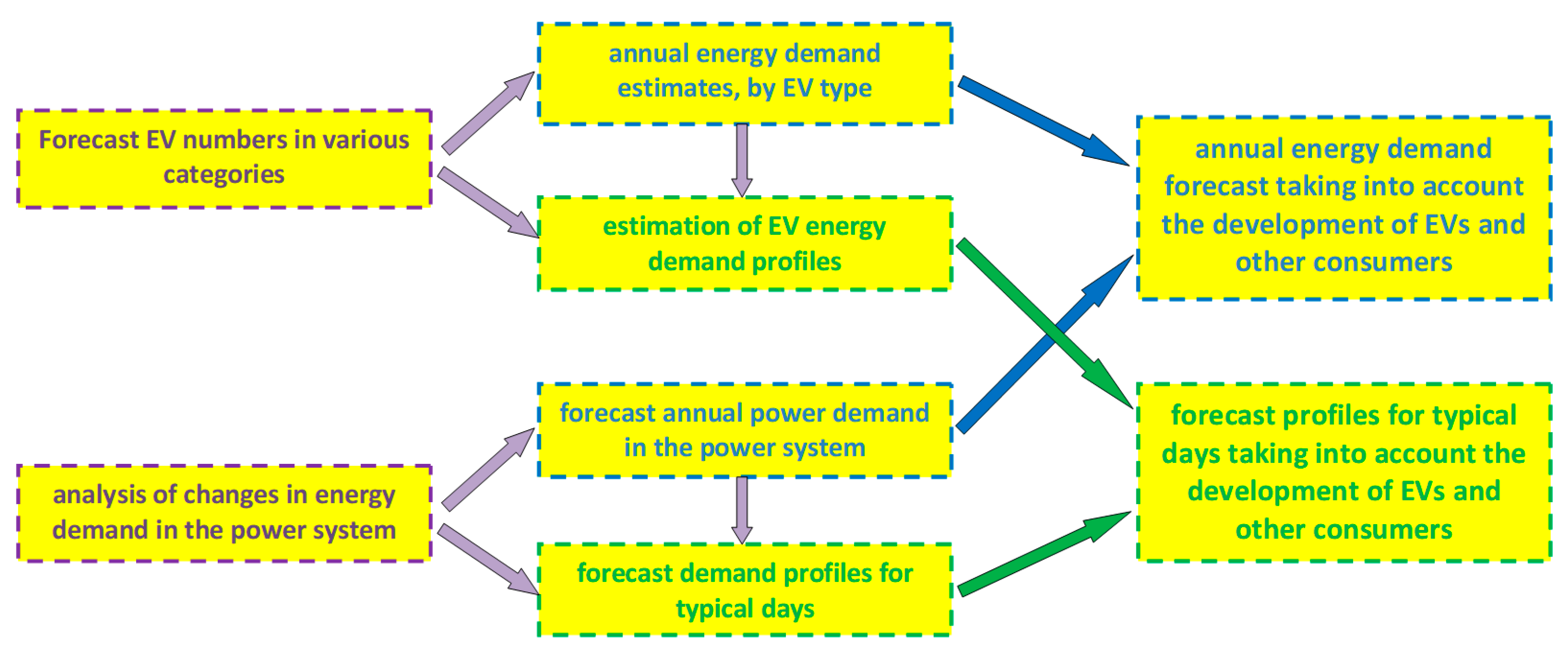
This section and its subsections describe forecasting methods and results as particular forecasts of various kinds were performed, until the final objective was achieved, that being forecast shapes of profiles until 2027 taking into account e-mobility development. The following models and methods were applied to particular forecasts, including: trend extrapolation models, methods based on time series, methods based on deterministic chaos theory, artificial neural networks (MLP and LSTM), as well as ensemble methods. The general diagramme of the studies described in this paper is shown in Figure 4.

3.1. Evaluation Criteria

To assess the quality of particular forecasting models within their parameter estimation ranges (availability of observed and forecast values), the following five evaluation criteria were used: Root Mean Square Error (RMSE) and Mean Absolute Percentage Error (MAPE) as the main evaluation criteria, Mean Bias Error (MBE), Pearson coefficient of linear correlation (R) and R-squared (R²) as three auxiliary evaluation criteria. It is worthwhile to note that the least RMSE and MAPE errors in the parameter estimation range do not mean that the model would generate the most accurate “ex ante” (forward-looking) forecasts. On the one hand, relatively small errors within the parameter estimation range are desirable (it would mean that the process has been well framed as a function of time). On the other hand, extremely small errors would mean that the model was unable to generalise (forecasts matching observed values too tightly, which would result in lower prognostic potential of such a model). Expert assessment of the magnitude of error was therefore required to select the preferred prognostic models.

Root Mean Square Error was calculated by Formula (1). RMSE is sensitive to large errors and is more useful when large errors are particularly undesirable.

$$RMSE=\sqrt{\frac{1}{n}{\displaystyle \sum }_{i=1}^n{(y_i-{\widehat{y}}_i)}^2}$$

(1)

where, ${\widehat{y}}_i$ is the predicted value, $y_i$ is the observed value, and n is the number of prediction points.

Mean Absolute Percentage Error is calculated by Formula (2).

$$MAPE=\frac{1}{n}{\displaystyle \sum }_{i=1}^n\left|\frac{y_i-{\widehat{y}}_i}{y_i}\right|\cdot 100\%$$

(2)

Mean Bias Error captures the average bias in the prediction, and is calculated by Formula (3)

$$MBE=\frac{1}{n}{\displaystyle \sum }_{i=1}^n\left(y_i-{\widehat{y}}_i\right)$$

(3)

Pearson coefficient of linear correlation between observed and predicted data was calculated by Formula (4). The forecasting method overestimates values if MBE < 0 or underestimates values if MBE > 0. The MBE error of a properly functioning prognostic method should be equal or very close to zero.

$$R=\frac{C_{y\widehat{y}}}{std\left(y\right)\cdot std\left(\widehat{y}\right)}$$

(4)

where, $C_{y\widehat{y}}$ s the covariance between the observed and predicted data, and std denotes standard deviation of the variable.

The bigger the error R (range from −1 to 1), the more accurate the prediction results.

R-squared was calculated by Formula (5).

$$R^2=1-\left(\left({\displaystyle \sum }_{i=1}^n{\left(\widehat{y_i}-y_i\right)}^2\right)/\left({\displaystyle \sum }_{i=1}^n{\left(y_i-\overline{y}\right)}^2\right)\right)$$

(5)

where, $\overline{y}$ is the mean of the observed load values.

The R-squared formula describes the difference between the goodness of fit of perfectly fitting model and models the sum of squared errors related to the sum of squared deviations of measured values from the mean value. The bigger R-squared is (range from 0 to 1) the better the model’s fit is and the more the process is explained by it. R-squared value gets lower with increasing concentration of the observed data around the mean value.

3.2. Forecast Number of Electric Vehicles in POLAND from 2022 to 2027

A very short time series of the cumulative number of EV registrations in Poland (period 2010–20121) increases the uncertainty of forecasts and justifies the use of an ensemble model based on several models. The process was assumed to be in its inception phase. The process growth dynamics (cumulative number of registered EVs) was strongly non-linear. A similar trend is also evident in other countries.

The methods used for forecasting EV numbers can also be grouped as follows: methods with control of the process growth ceiling (logistic function and a Model According to Prigogine) and methods without control of the process growth ceiling (other methods). It is worthwhile noting that the process reviewed here would not be growing indefinitely. At some point, the process would reach its ceiling. This is due to the fact that the number of vehicles (regardless of their power source) in a country would not grow indefinitely, and would strongly depend on the size of the population.

Table 1. Groups of methods used for forecasting the number of electric vehicles.

Name of Method	Equation No.	Model Parameter Optimisation Method	Minimised Error	Step Forecasts
Category I. Methods of direct trend extrapolation
Logistic function *	(6)	Differential Evolution and Particle Swarm Optimisation algorithm (DEPS)	Sum of Squared Errors (SSE)	No
Exponential function	(7)	Method of Least Squares (MLS)	SSE	No
MLP artificial neural network	-	Broyden–Fletcher–Goldfarb–Shanno algorithm (BFGS)	SSE	No
Category II. Methods based on deterministic chaos theory
Model According to Prigogine *	(8)	DEPS	SSE	Yes
Category III. Methods using time series
Grey Model GM(1,1)	(9)	DEPS	SSE	Yes
Growth Dynamics Model	(10)	MLS	SSE	Yes
Category IV. Method using more than one model
Ensemble Model	(12)	-	-	No

Remark: * growth ceiling control models.

shows the grouping of the methods used for forecasting the number of electric vehicles.

The extrapolation model of the logistic function was described by Formula (6) [24].

$$y\left(t\right)=\frac{a}{1+b\cdot e^{-c\cdot t}}$$

(6)

where, $t$ is the sample index in the time series of the process,$a>0$ is the saturation level and $b>0, c>0$ are the parameters. The saturation level is adopted to be exactly 15 million—in Poland, more than 24 million vehicles of all power-source types are registered (about 750 vehicles per 1000 inhabitants).

The extrapolation model of the exponential function was described by Formula (7).

$$y\left(t\right)=a\cdot e^{b\cdot t}$$

(7)

where, $a,b$ are the parameters.

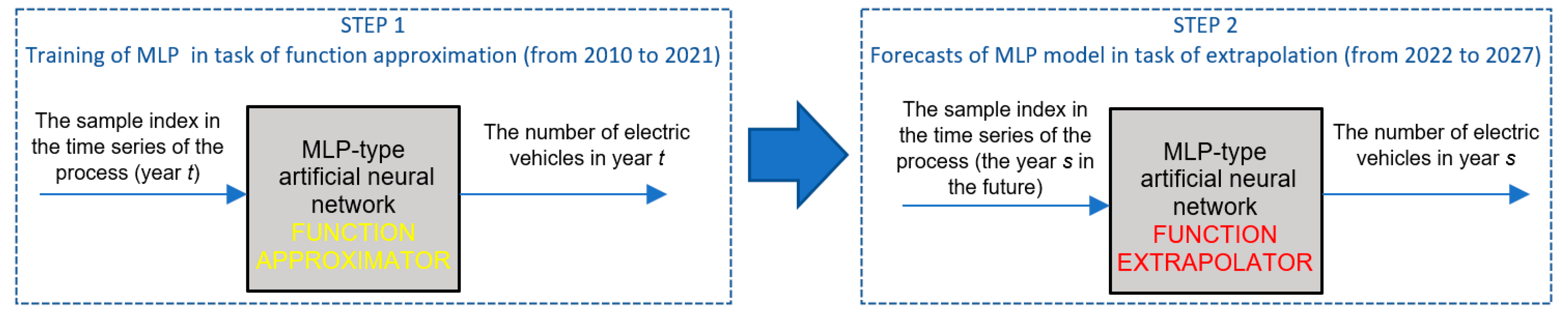
The application of the MLP artificial neural network to the extrapolation exercise is our original, unique proposition to use ANN. MLP is typically used in regressive (including forecasting [30,31]) and classification problems [32] and requires a large number of learning modules. In this case, MLP was first used for the construction of non-linear function, or the approximation exercise. In this case there was no explicit function formula, rather it was embedded in the architecture of the neural network, in the weights (parameters) and functions of activation of particular layers of the neural network. Next, MLP was applied to forecast out-of-range values (extrapolation). Figure 5 presents a diagram of subsequent actions using an MLP neural network to obtain the forecast number of EVs.

Tests for various hyperparameters were performed to select appropriate models.

The tested number of hidden neurons ranged from 1 to 4. The number of learning epochs was tested for the following values: 10, 20, 50, 100, 150 and 200. The number of learning epochs had a large influence on the level of “smoothing out” of the function being approximated. With too large a number of learning epochs, MLP learned the values too strictly, thus, losing the capacity to generalise. For the hidden layer, the Linear and Exponential activation functions were tested. In the baseline layer, the exponential activation function was adopted as the one appropriate for the process studied. Such a choice ensured that the MLP neural network was capable of extrapolating (able to predict outside of the learning range). As a result of extensive tests, outcomes of the forecasts of two MLP models were finally selected. Both models had one input and one output. To optimise the weights (model parameters), BFGS optimisation algorithm was applied.

The first of the selected models had 2 hidden neurons and an exponential activation function in the hidden layer and in the output layer (MLP 1-2-1 (exp/exp)).

The other selected model had 2 hidden neurons and a linear activation function in the hidden layer, and exponential activation function in the output layer (MLP 1-2-1 (linear/exp)). Both models were learning for 100 learning epochs, with weights being updated following each learning epoch.

The Model According to Prigogine was described by Formula (8) [28,29].

$$y\left(t\right)=y\left(t-1\right)\cdot \left[1+r\cdot \left(1-\frac{y\left(t-1\right)}{K}\right)\right]$$

(8)

where y$\left(t\right)$ is the population size in period $t$, $r>0$ is the population growth rate, $K>0$ is the development ceiling (forecast population growth in the future). The development ceiling was assumed to be 15 milion.

Grey Model GM (1,1) was described by Formula (9) [24]. In this model, the order of the Grey Differential Equation and the number of variables are equal to 1. This model is recommended by literature [33], especially for very short time series and where the process evolution is in its initial phase.

$$\begin{gathered} \widehat{y}\left(t\right)={\widehat{y}}^{\left(1\right)}\left(t\right)-{\widehat{y}}^{\left(1\right)}\left(t-1\right), \\ {\widehat{y}}^{\left(1\right)}\left(t\right)=\left[y^{\left(1\right)}\left(1\right)-\frac{u}{a}\right]\cdot e^{\left(-a\left(t-1\right)\right)}+\frac{u}{a} \\ {\widehat{y}}^{\left(1\right)}\left(t\right)={\displaystyle \sum }_{i=1}^{t}y\left(i\right), t=1,2,\dots ,n \end{gathered}$$

(9)

where $n\ge 4$ is the length of time series, $a$ is the evolution parameter, $u$ is the grey variable and $\widehat{y}\left(t\right)$ is the forecast in period t.

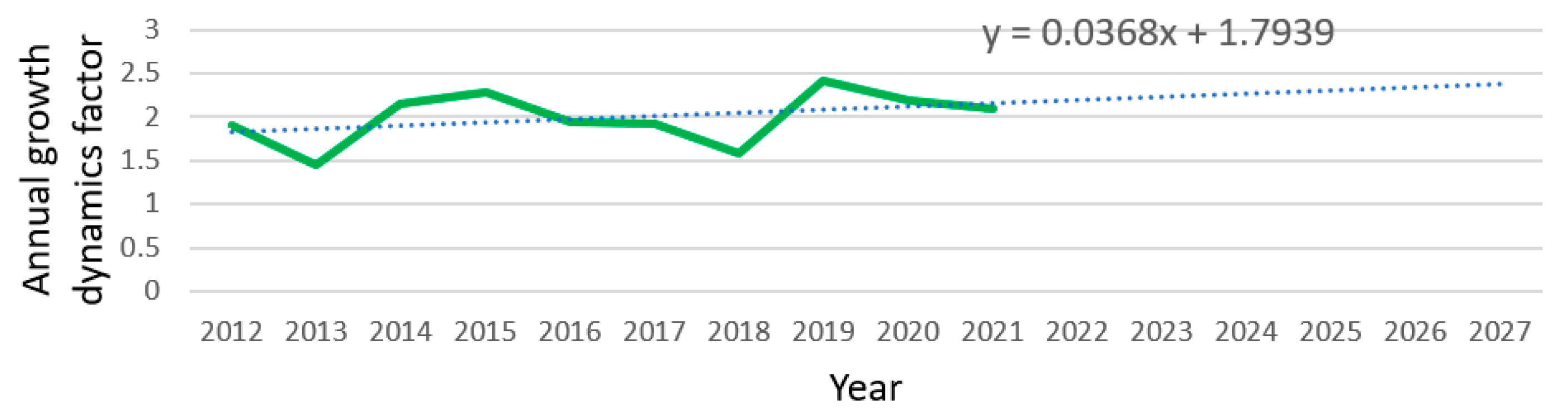
The Growth Dynamics Model is our original, unique proposal for a model. In Step One, annual growth rates were calculated for 2011–2021 as the rate of the number of EVs in the year to the number of EVs in the prior year. In Step Two, annual growth rates were approximated to a linear function. Figure 6 presents the variability of annual growth rates.

Formula (10) presents a linear function equation with calculated parameter values.

$$c_{growth}\left(t\right) = 0.0368\ast t+1.7939$$

(10)

In Step Three, annual growth rates for 2022–2027 were forecast, using extrapolation of the linear function onto subsequent periods (forward-looking). In Step Four, appropriate stepwise forecasts of the number of EVs were conducted for 2022–2027, using the calculated forecast annual growth rates. Forecast number of EVs was calculated for each year according to Formula (11)

$$y\left(t\right)=y\left(t-1\right)\ast {\widehat{c}}_{growth}\left(t\right)$$

(11)

where, $y\left(t\right)$—forecast number of EVs in period t, ${\widehat{c}}_{growth}\left(t\right)$—forecast annual growth rate for period t, calculated as extrapolation of the linear function.

The Ensemble Model was described by Formula (12) [24]. The forecast in the Ensemble Model was the weighted arithmetic average of forecasts from several models. To construct such a model, seven single prognostic models were used (logistic function, exponential function, MLP 1-2-1 (exp/exp), MLP 1-2-1 (linear/exp), Model According to Prigogine, Grey Model GM(1,1) and Growth Dynamics Model). Averaged results of forecasts from different models should increase reliability of forecasting.

$${\widehat{y}}_t=\frac{{{\displaystyle \sum }}_{i=1}^k{\widehat{y}}_t^i\cdot w_i}{{{\displaystyle \sum }}_{i=1}^k{w}_i}, w_i=\frac{1}{k}$$

(12)

where k is the number of forecasting models and ${\widehat{y}}_t^i$ is the forecast in period t generated by the model number i.

Table 2. Performance metrics in the model’s parameter estimation range for the forecast number of EVs.

Method Name	RMSE	MAPE [%]	MBE	R	R2
MLP 1-2-1 (exp/exp)—pessimistic variant	4.13	15.26	54.53	0.99983	0.99962
Logistic function	15.61	16.83	39.34	0.99982	0.99963
Exponential function	16.06	16.67	38.33	0.99982	0.99962
MLP 1-2-1 (linear/exp)	18.97	9.28	20.34	0.99982	0.99964
Ensemble model—balanced variant	34.99	9.83	31.15	0.99975	0.99950
Model According to Prigogine	93.41	12.62	−17.70	0.99898	0.99797
Grey Model GM(1,1)	249.29	11.08	131.74	0.99980	0.99907
Growth Dynamics Model—optimistic variant	346.09	10.78	−47.22	0.99884	0.99729

Remarks: The best fitting results for each fitness metric are printed in bold in blue. The worst fitted result is printed in red.

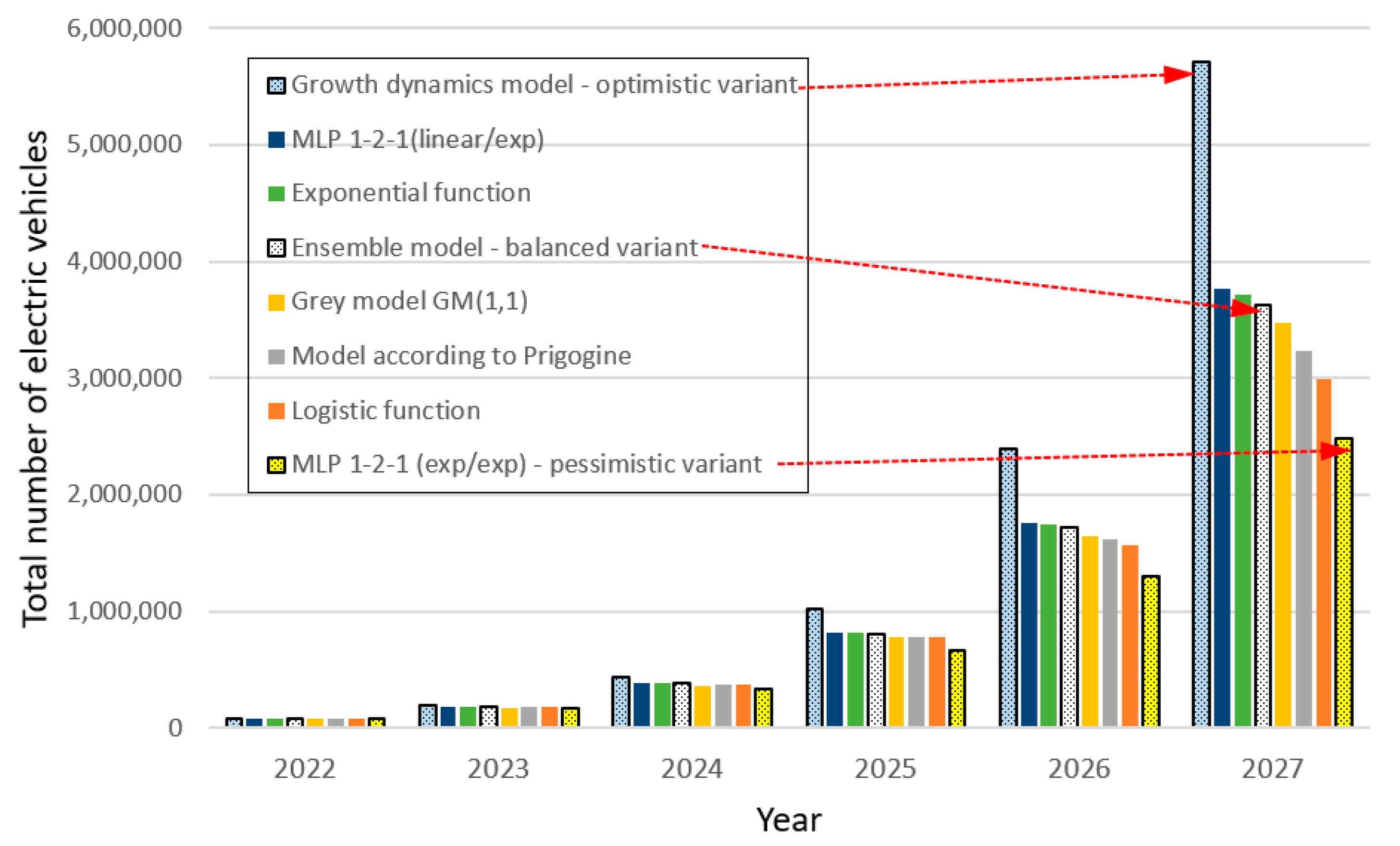
presents summary results (quality assurance metrics) for the model’s parameter estimation range (2010–2021). Figure 7 presents the results of forward-looking (2022–2027) forecasts of the total number of EVs in Poland for the eight methods.

The best fitting model for historical data was MLP 1-2-1 (exp/exp) model. It was selected as the pessimistic variant (the lowest “ex ante” forecast values (2022–2027)). The Growth Dynamics Model was the least fitting model in the parameter estimation range. This model was selected as the optimistic variant (largest “ex ante” forecast values (2022–2027)). The Ensemble Model was selected as the most credible model for a balanced model.

The pessimistic and optimistic variants were the models that differed the most from the remaining models, in terms of forecast values. This effect was particularly evident for the 2027 forecasts.

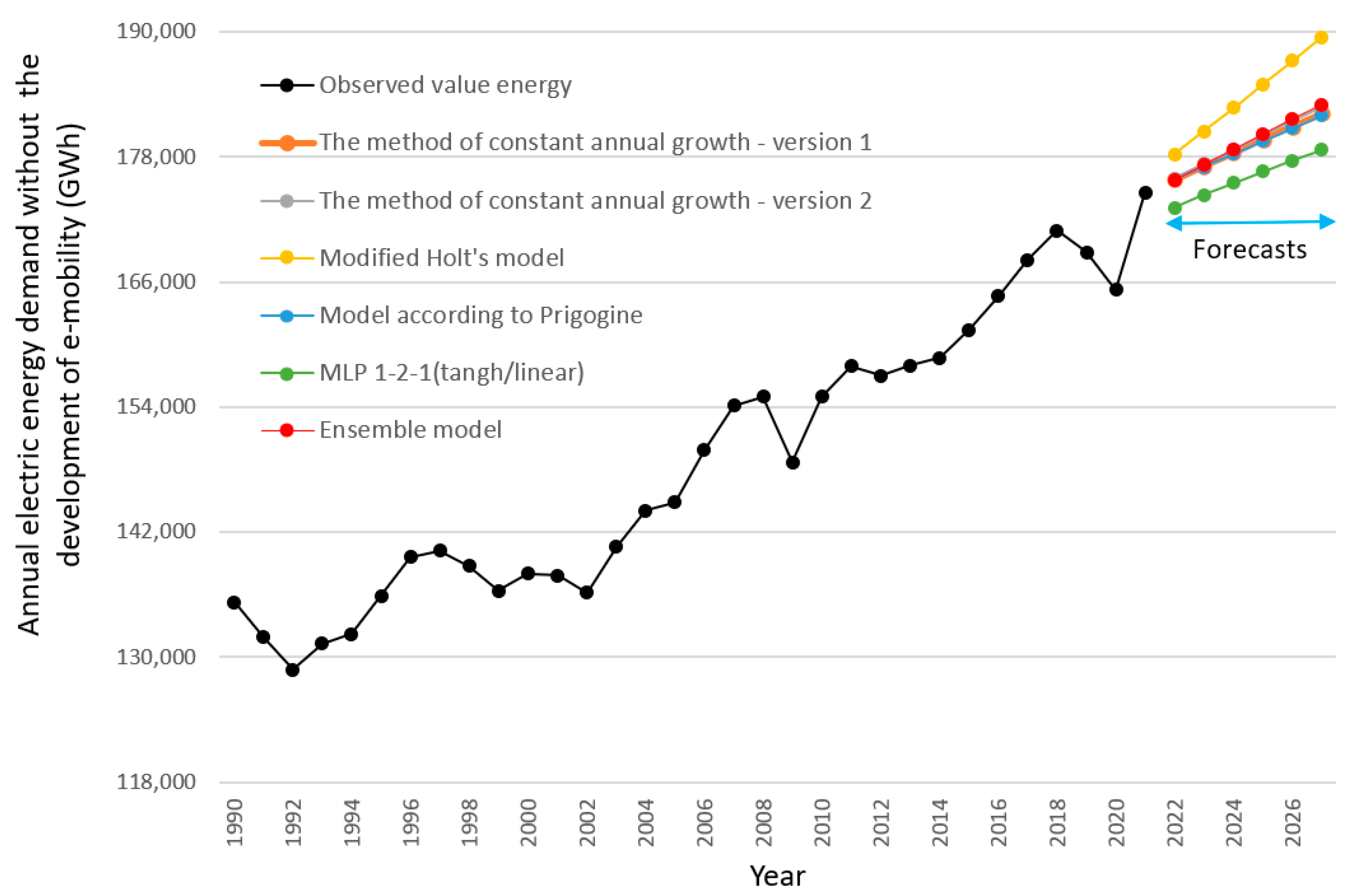
3.3. Forecast Annual Power Demand in Poland from 2022 to 2027 Excluding the Development of E-Mobility in Poland

Forecasts of annual demand for power with the exclusion of e-mobility were conducted by six methods.

The first model, a modified Holt’s model, is presented in detail in [34]. Model parameters for the data from the estimation range (1991–2021) were selected using optimisation by the DEPS method. The minimum SSE was sought. Forecasts were conducted by a Stepwise Method (2022–2027).

The second model, the Model According to Prigogine was described by Formula (8). Model parameters for the data from the estimation range (1991–2021) were selected using optimisation by the DEPS method. The minimum SSE was sought. Forecasts were conducted by a Stepwise Method (2022–2027).

The third model, the Method of Constant Annual Growth, Version 1, was described by Formula (13). Annual growth was the average annual growth rate based on historical data of the forecasting exercise. Forecasts were conducted by a Stepwise Method (2022–2027).

$${\widehat{y}}_t={\widehat{y}}_{t-1}+\frac{{{\displaystyle \sum }}_{j=2}^k\left(y_j-y_{j-1}\right)}{k-1}$$

(13)

where k is the number of the data points in the time series and $y_{j-1}$ is the previous value (or forecast) from the time series.

The fourth model, the Method of Constant Annual Growth, Version 2, was described by Formula (14). Annual growth was equal to the slope A from the linear function used for the approximation of the trend line (1991–2021) of annual power demand. The parameter value was A = 1382.30. Forecasts were conducted by a Stepwise Method (2022–2027).

$${\widehat{y}}_t={\widehat{y}}_{t-1}+A$$

(14)

where, A—parameter from the linear function used for the approximation of the trend line.

The fifth model was an original, unique proposed model, MLP Artificial Neural Network. The model was described (conceptually) in Section 3.2. To select the appropriate model, tests for various hyperparameters were conducted. The tested number of hidden neurons ranged from 1 to 3. The number of learning epochs was tested for the following values: 5, 10, 20 and 50. The number of learning epochs had a large influence on the level of “smoothing out” of the function being approximated. For the hidden layer, the Linear and Hyperbolic Tangent activation functions were tested. In the output layer, a Linear activation function was adopted as the one appropriate for the process studied here, which was due to the variability of the forecast process. Such a choice ensured that the MLP neural network was capable of extrapolating (able to predict outside of the learning range). To optimise the weights (model parameters), the BFGS optimisation algorithm was applied. The selected final mode had two hidden neurons and Hyperbolic Tangent activation function in the hidden layer, and a Linear activation function in the output layer (MLP 1-2-1 (tangh/linear). This model learned for 10 learning epochs, with weights updated following each learning epoch.

The sixth model, the Ensemble Model, was described by Formula (12). The following methods were selected for the ensemble model: Modified Holt’s Model, Model According to Prigogine, Constant Annual Growth Method, Version 1, Constant Annual Growth Method, Version 2, and MLP 1-2-1 (tangh/linear).

Table 3. Performance metrics for the forecast values of annual power demand in Poland within the model’s parameter estimation range.

Method Name	RMSE	MAPE [%]	MBE	R	R2
MLP 1-2-1 (tangh/linear)	509.04	1.574	−112.04	0.9776	0.9556
Ensemble model	1402.67	1.571	152.27	0.9753	0.9510
Constant Annual Growth Method—Version 2	1658.21	1.755	−114.49	0.9693	0.9393
Constant Annual Growth Method—Version 1	1665.56	1.751	−5.6 × 10−12	0.9693	0.9393
Model according to Prigogine	1665.76	1.751	−2.18	0.9694	0.9394
Modified Holt’s Model	1692.48	1.776	990.05	0.9681	0.9253

Remarks: The best fitting results for each fitness metric are printed in bold in blue. The worst fitted result is printed in red.

presents summary results (quality assurance metrics) for the model’s parameter estimation range (1991–2021). Figure 8 presents the time series of the observed annual power demand figures in Poland and results of forecasts from 2022 to 2027, obtained by the six methods.

MLP 1-2-1 (tangh/linear) was the model that best fit the historical data, and at the same time it generated the lowest values of “ex ante” forecasts (2022–2027). The least fitting model in the parameter estimation range was the Modified Holt’s model, and at the same time it generated the largest “ex ante” forecast values (2022–2027). Results of forecasts from the Ensemble Model were selected for further analyses.

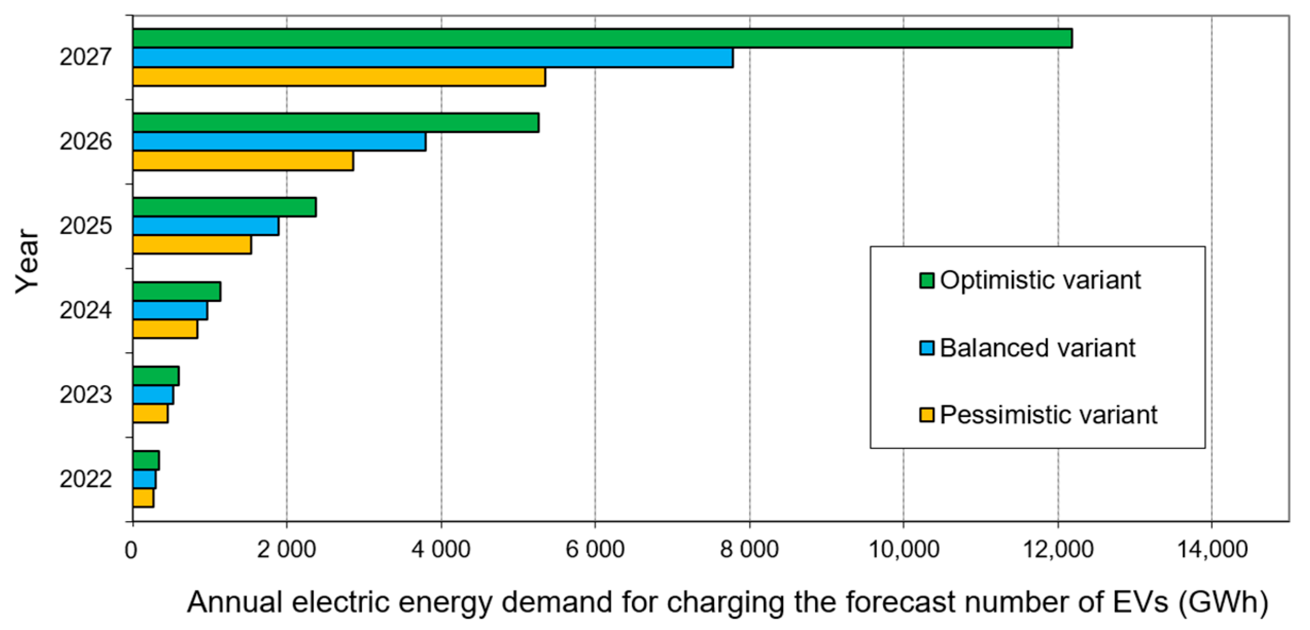
3.4. Forecast Annual Power Demand in Poland from 2022 to 2027 Solely due to the Operation of the Forecast Number of EVs

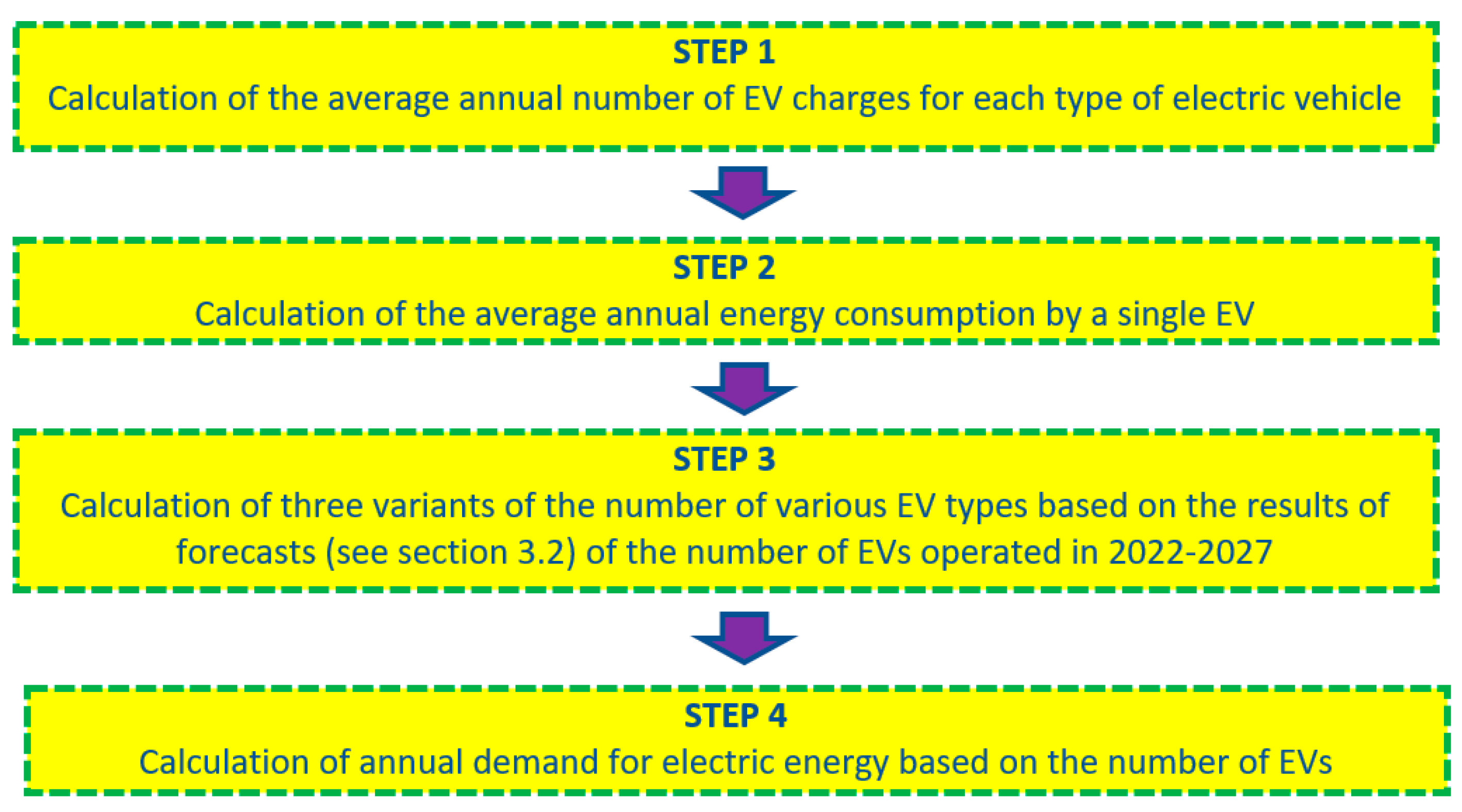
The algorithm had four steps. Figure 9 shows the details.

Table 4. Input data and calculation results for 2027.

Description	BEVs	PHEVs	Electric Buses	Electric Trucks	Electric Delivery Vans
Input data for calculations
Average annual mileage [km]	15,000	10,000	80,000	80,000	80,000
Battery capacity in a single EV [kWh]	49.7	12.2	167.5	276.6	48.2
Average EV driving range [km]	343.6	61.2	175.0	252.2	260.0
Results of calculation of average values
Average annual number of charges	44	163	457	317	308
Average annual power consumption by a single EV [kWh]	2169.7	1993.5	76,571.4	87,727.2	14,830.8
Results of calculation of the number of EVs in 2027
Pessimistic variant [pcs]	1,217,911	1,262,651	1126	709	2849
Balanced variant [pcs]	1,777,612	1,842,912	1501	945	3799
Optimistic variant [pcs]	2,801,269	2,904,173	1876	1181	4749
Outcome of calculation of power demand for charging the forecast number of EVs in 2027
Pessimistic variant [GWh]	2642.5	2517.1	86.2	62.2	42.3
Balanced variant [GWh]	3856.8	3673.8	114.9	82.9	56.3
Optimistic variant [GWh]	6077.8	5789.4	143.7	103.6	70.4

contains input data and summary calculation results for 2027 (forecasts with six years’ horizon).

Battery capacity and average driving ranges of BEVs and PHEVs were determined as averages calculated for 38 and 65 different vehicle models, respectively, costing less than PLN 0.25 million. For electric vans, these variables were determined as average figures for 17 vehicles of that type. For electric buses, the range and battery capacity were adopted in accordance with [24].

For forecast number of electric trucks of various sizes and the number of electric buses in the six years’ horizon, constant growth of the number of vehicles was assumed (average growth from the last several years), such was the observed dynamics of both processes. Forecast numbers of BEVs and PHEVs in subsequent years were calculated as 49% and 51%, respectively, of the forecast values for the given year of the number of EVs of all categories (having deducted forecast number of vehicles from the remaining three categories).

The analysis of results from Table 4 showed that BEVs and PHEVs, or mainly passenger transport, would have by far the biggest impact on annual power demand in Poland in the next six years. For buses, the level of electrification would be about 16% of the fleet (currently, there are about 12,000 buses with various power-source variants). Electric trucks would have no significant impact on power demand, despite large battery capacities, due to the fact that their number in the next six years was not predicted to be very large. Electric delivery vans would probably be more significantly electrified, as the manufacturers’ offer gets bigger every year. For that reason, the calculations assumed a 75% share of those vehicles in the category of electric trucks of various sizes.

Figure 10 shows three variants of the forecast annual demand for power in Poland in 2022–2027, resulting solely from the operation of the forecast number of electric vehicles.

3.5. Forecast Annual Power Demand in Poland from 2022 to 2027 Taking into Account the Development of E-Mobility in Poland

The forecast value for the year was the sum of the forecast power demands, excluding e-mobility, for the year (for the result obtained from the Ensemble Model, details in Section 3.3) and the three variants of forecast power demand resulting from the operation of electric vehicles in the year (details in Section 3.2). The results of calculations are presented in

Table 5. Results of calculations of power demand with e-mobility, in three variants.

	Power Demand Without e-Mobility	Power Demand with E-Mobility
Year	Ensemble Model [GWh]	Pessimistic Variant [GWh]	Balanced Variant [GWh]	Optimistic Variant [GWh]
2022	175,799	176,063	176,098	176,135
2023	177,272	177,734	177,795	177,865
2024	178,733	179,566	179,702	179,873
2025	180,180	181,718	182,067	182,557
2026	181,615	184,481	185,415	186,882
2027	183,038	188,389	190,824	195,224

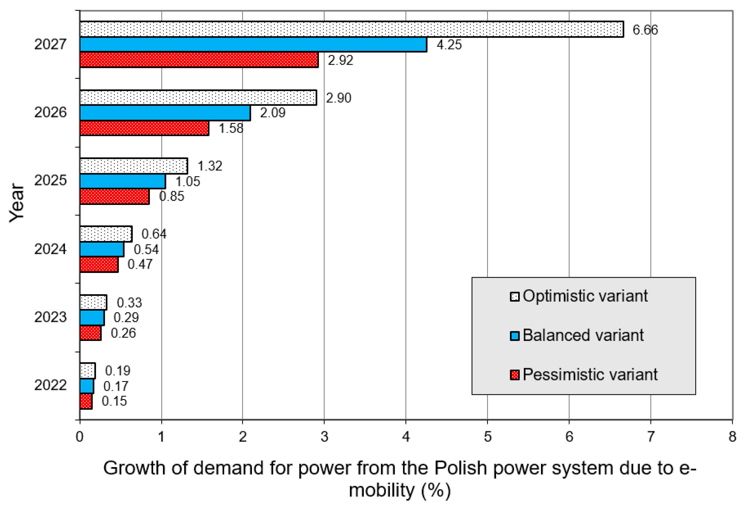
. Figure 11 shows, for the three variants the forecast percentage growth of power demand due to e-mobility in Poland from 2022 to 2027.

The results in Table 5 and Figure 11 show that, for the initial period (forecasts for 2022–2024), the impact of e-mobility on the Polish electric power system was negligible. In subsequent years (forecasts for 2023–2027), the impact of e-mobility on the Polish power system grew dynamically, reaching almost 7% for the optimistic variant. Such an extra annual amount of power (more than 12 [TWh]) is a big challenge for the Polish electric power system, especially in the context of the energy crisis (energy deficit). On the other hand, the mechanisms of the “Fit for 55” package (phasing out manufacturing of petrol or diesel vehicles) means that significantly larger quantities of power need to be generated to meet the e-mobility demand (EV charging). Obviously, these will be covered by RES to some extent.

3.6. Forecast Daily Profiles of Typical Days in 2022–2027 without E-Mobility

The third Wednesday of July and the third Wednesday of January are “typical days” in the Polish Power System, representing the summer and the winter business days, respectively. Forecasts for both relative daily profiles (normalised hourly values) were conducted for both typical days with a horizon of six years (2022–2027). The normalisation procedure is described in Section 2. Normalisation enabled us to the track changes in the profiles over 2009–2021, ignoring any profile change resulting from a multi-annual growing trend of power demand in the subsequent years.

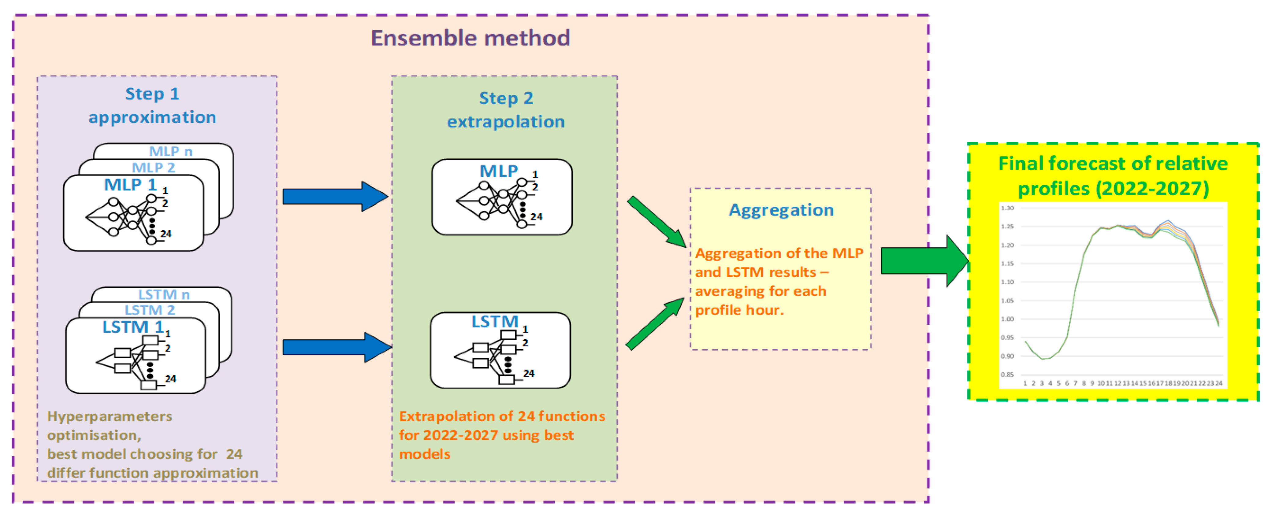
Forecast relative values of the profiles in the subsequent years, conducted separately for each hour, used the following methods: MLP-type Artificial Neural Network, LSTM-type Deep Neural Network (DNN) and Ensemble Model (final forecast).

Both the MLP and LSTM were used in Step One for simultaneous approximation of 24 different functions (variability of demand for power for the respective hour of the day between 2009 and 2021) in a single model of artificial neural network with 24 outputs (function values) and 1 input (sample index in the time series of the process). In the next step, relative values of both profiles were forecast by extrapolating the function onto six consecutive periods (from 2022 to 2027). The use of an artificial neural network for extrapolation of the function is our original, unique ANN application proposal. Figure 12 conceptually presents our unique method using two different models of neural networks.

The first model used in the Ensemble Model was MLP. The model is described (conceptually) in Section 3.2. Tests for various hyperparameters were performed to select appropriate models. The tested number of hidden neurons ranged from 3 to 12. The number of learning epochs was tested for the following values: 10, 20, 30, 40 and 50. The number of learning epochs had a large influence on the level of “smoothing out” of the function being approximated. For the hidden layer, a hyperbolic tangent was selected as the activation function. Linear activation function in the output layer was adopted as the appropriate one for the process studied here. Such a choice ensured that the MLP neural network was capable of extrapolating (able to predict outside of the learning range). To optimise the weights (model parameters), the BFGS optimisation algorithm was applied. The finally selected models for forecasting the typical winter and summer day profiles had six neurons in the hidden layer (MLP 1-6-24 (tangh/linear)). Both models were learning for 20 learning epochs, with weights being updated following each learning epoch.

The other model applied in the Ensemble Model was LSTM. The model is described in [35]. Tests for various hyperparameters were performed to select appropriate models. The number of hidden neurons was tested in the range between 3 and 50. The number of learning epochs was tested for the following values: 50, 100, 200, 300 and 500. For the hidden layer, Sigmoid, Relu, and Hyperbolic Tangent activation functions were tested. Linear function was applied in the output layer. Adaptive Moment (Adam) and Root Mean Square Propagation (RMSprop) Optimisation Algorithms were tested to optimise the weights. In addition, the Dropout technique, with the value of 0.1 along the hidden layer, was applied, and the absence of that mechanism was tested. Both final models, selected by expert choice, were taught for 200 epochs, with the Sigmoid function in the hidden layer without the Dropout technique, and with the Adam (winter profile) and RMSPprop (summer profile) optimisation algorithms. The finally selected models for forecasting the profiles of typical days in January (LSTM 1-3-24 (sigm/linear)) and in July (LSTM 1-4-24 (sigm/linear)) had 3 and 4 neurons in the hidden layer, respectively.

The appropriate models (MLP, LSTM) were selected by expert choice based on the size of errors in the estimation range, and the observation of the level of “smoothing out” of forecasts within the model’s parameter estimation range (the model should preserve a non-linear shape of forecasts with simultaneous avoidance of overestimating).

The application of two independent non-linear models was much more accurate than a simple linear regression model, for example, in terms of extrapolating forecasts independently for each hour. The linear model was unable to reflect the non-linear shape of the variability of power demand in the respective hour over consecutive years. To apply linear regression, one needs to build 24 independent models for the given typical day, whereas a single neural network generates 24 values of the typical day profile simultaneously in a single step. Such a simplified linear approach to the forecast profiles was applied in [24]. 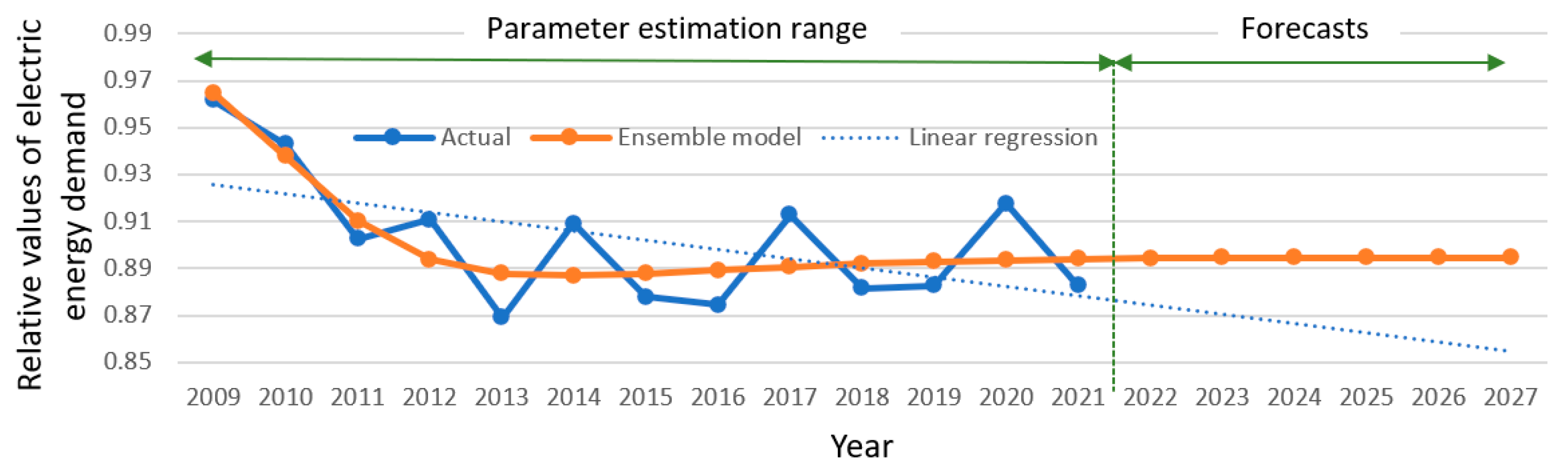Figure 13 presents differences in the operation of the linear model of regression with trend extrapolation, and the proposed non-linear Ensemble Model. The shapes of forecast curves of the Ensemble Model were clearly non-linear (especially for the estimation of model parameters). The Linear Regression (LR) Model clearly underestimated forecasts in 2022–2027, as compared to the Ensemble Model, as it failed to incorporate a significant change in the downward trend in the last years of the model’s parameter estimation range (2014–2021). Process figures from recent years should weigh more since they reflect the most current status of the process trend line. The figures presented in Figure 13 indicated that the process had stabilised (cessation of the downward trend).

Table 6. Summary of forecast relative profiles of typical days for three models (error metrics) within the models’ parameter estimation range (2009–2021).

Method Name	RMSE	MAPE [%]	R	R2
Relative profile of the winter typical day
MLP 1-6-24 (tangh/linear)	0.0172	1.300	0.7447	0.5649
LSTM 1-3-24 (sigm/linear)	0.0197	1.423	0.7094	0.4180
Ensemble Model	0.0179	1.311	0.7345	0.5285
Relative profile of the summer typical day
MLP 1-6-24 (tangh/linear)	0.0110	0.922	0.7726	0.6091
LSTM 1-4-24 (sigm/linear)	0.0128	0.970	0.7191	0.5116
Ensemble model	0.0116	0.931	0.7532	0.5865

presents aggregate results of relative forecast profiles of typical days for the three models (error metrics) in the models’ parameter estimation range (2009–2021). Error metrics were average values calculated on errors obtained separately for each of the 24 h of the given profile. The error metrics thus obtained indicated that, within the estimation range, the models were better fitted, in terms of relative profile of the typical day, for the summer rather than for the winter. Detailed summary of the results (five error metrics) for each separate hour is provided in

Table A1. Forecast accuracy metrics of the MLP + LSTM Ensemble Method for particular times of the day.

	Relative Profile of the Winter Typical Day					Relative Profile of the Summer Typical Day
Hour *	RMSE	MAPE [%]	MBE	R	R2	RMSE	MAPE [%]	MBE	R	R2
1	0.0165	1.383	0.00430	0.8054	0.6212	0.0094	0.907	0.00142	0.6934	0.4680
2	0.0151	1.410	0.00245	0.8350	0.6877	0.0090	0.950	0.00185	0.7131	0.4849
3	0.0149	1.356	0.00349	0.8468	0.7004	0.0098	0.971	0.00249	0.6526	0.3751
4	0.0158	1.394	0.00396	0.8208	0.6501	0.0092	0.928	0.00134	0.6770	0.4251
5	0.0159	1.412	0.00270	0.7932	0.6176	0.0098	0.994	0.00148	0.7337	0.5241
6	0.0167	1.446	0.00296	0.7397	0.5315	0.0116	1.029	0.00251	0.7878	0.5914
7	0.0196	1.450	0.00362	0.5105	0.2327	0.0092	0.805	0.00056	0.9346	0.8718
8	0.0221	1.521	0.00423	0.5153	0.2367	0.0092	0.752	0.00084	0.9314	0.8662
9	0.0200	1.393	0.00306	0.5647	0.3020	0.0116	0.862	0.00134	0.8591	0.7341
10	0.0187	1.308	0.00459	0.6331	0.3616	0.0118	0.886	0.00198	0.8074	0.6417
11	0.0171	1.141	0.00619	0.7159	0.4386	0.0123	0.885	−0.00063	0.7491	0.5597
12	0.0165	1.135	0.00353	0.6888	0.4470	0.0120	0.882	0.00030	0.7581	0.5744
13	0.0168	1.131	0.00408	0.6769	0.4210	0.0127	0.931	−0.00081	0.7715	0.5928
14	0.0177	1.131	0.00048	0.6820	0.4646	0.0132	0.982	0.00058	0.7567	0.5714
15	0.0189	1.261	0.00542	0.6262	0.3375	0.0133	0.990	−0.00022	0.7603	0.5777
16	0.0186	1.194	0.00486	0.5862	0.2955	0.0134	1.013	−0.00007	0.8209	0.6734
17	0.0201	1.283	0.00210	0.7187	0.5094	0.0142	1.067	0.00102	0.8241	0.6771
18	0.0200	1.296	0.00234	0.8283	0.6810	0.0153	1.064	0.00298	0.8001	0.6249
19	0.0190	1.253	0.00006	0.8441	0.7125	0.0152	1.067	0.00187	0.8191	0.6614
20	0.0197	1.312	−0.00033	0.8511	0.7242	0.0125	0.947	0.00141	0.8778	0.7651
21	0.0197	1.370	0.00407	0.8343	0.6818	0.0114	0.871	0.00128	0.8521	0.7226
22	0.0176	1.279	0.00388	0.8565	0.7189	0.0108	0.769	−0.00049	0.5679	0.3095
23	0.0164	1.284	0.00578	0.8479	0.6775	0.0105	0.858	0.00135	0.4894	0.4010
24	0.0152	1.322	0.00327	0.8063	0.6322	0.0105	0.930	0.00047	0.4407	0.3820

* Hour corresponds to the point in time of measurement/end of hourly period, e.g., hour = 12 corresponds to 11:00–12:00 period.

in Appendix A.

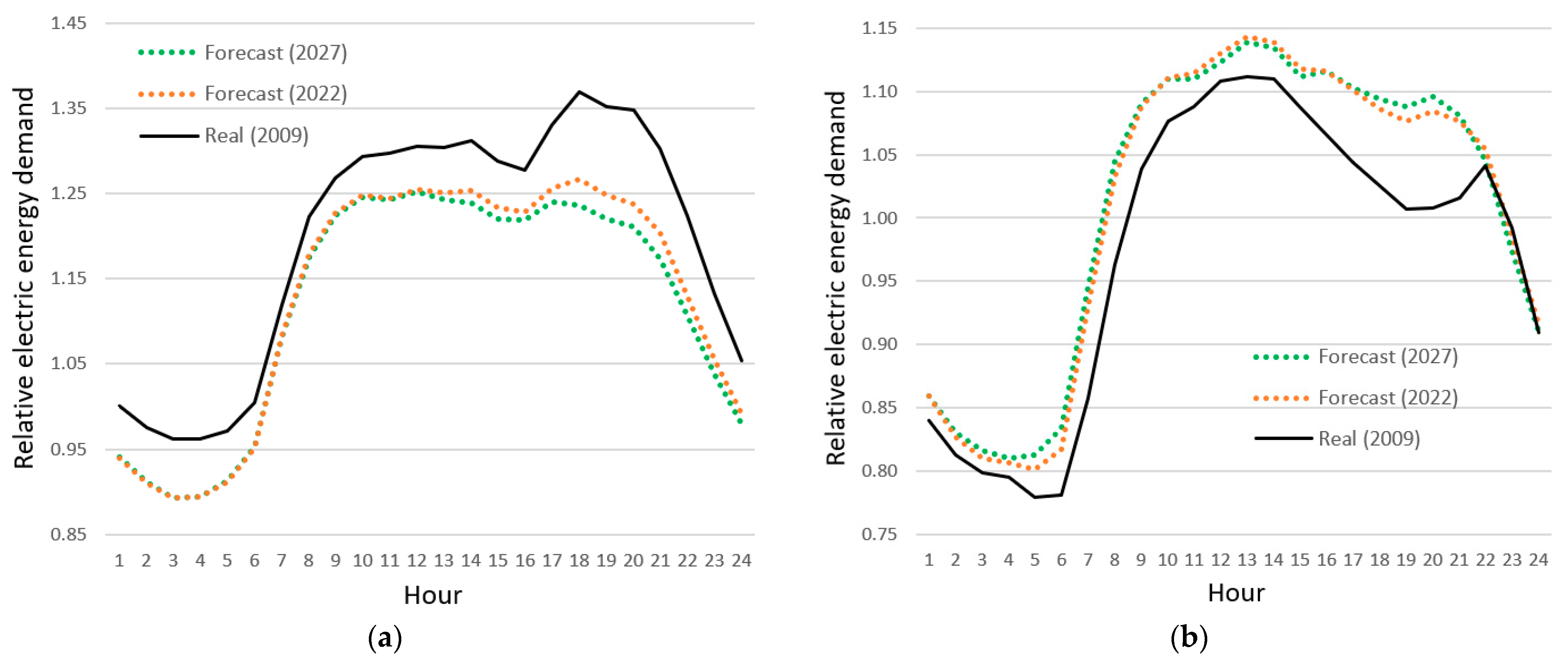
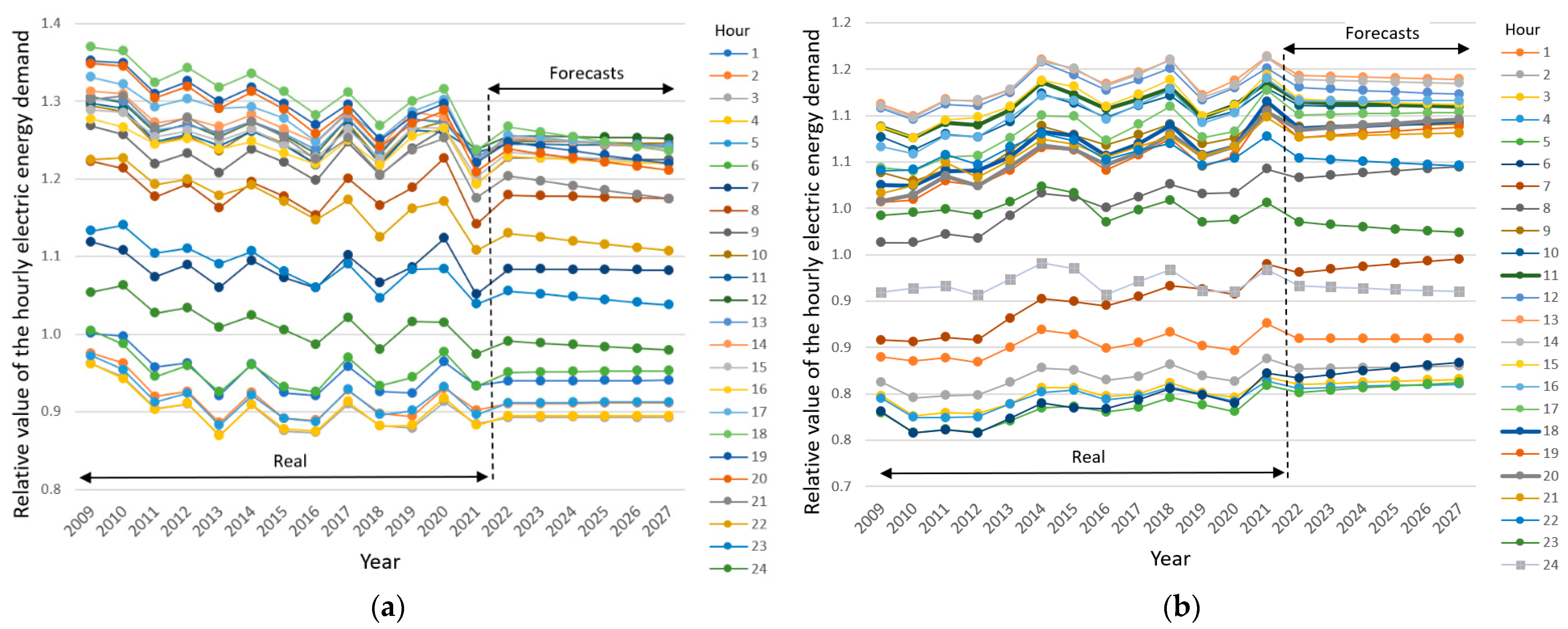
Figure 14 presents forecast power demand in particular hours of the typical winter and summer days (2022–2027), and observed values (2009–2021). Figure 15 presents forecast relative profiles of power demand for the typical winter and summer days. The trend of change in relative demand varied by hour. For the profile of the winter typical day, relative power demand slightly fell in particular hours between 01:00 pm and 12:00 pm between the last year of the forecast (2027) and the first year of the forecast (2022). In the night “valley”, profile changes were minimal.

For the profile of the summer typical day, there were both slight increases in demand for power in the night “valley” of daily demand, and in the evening “peak” of power demand. In the morning “peak”, power demand fell slightly.

3.7. Forecast Daily Profiles of Typical Days in 2022–2027 with E-Mobility

In Step One, calculations were conducted to transform the forecast values of relative power demand profiles (2022–2027) into absolute values of power demand. Relative forecast values of both profiles (2022–2027) (details in Section 3.6) were recalculated to absolute values [GWh]. However, forecast annual power demand in Poland (2022–2027), as detailed in Section 3.3, was recalculated to obtain average hourly figures of power demand during that year. This method incorporated both the growing trend of the annual power demand and how relative profiles evolved over the subsequent years.

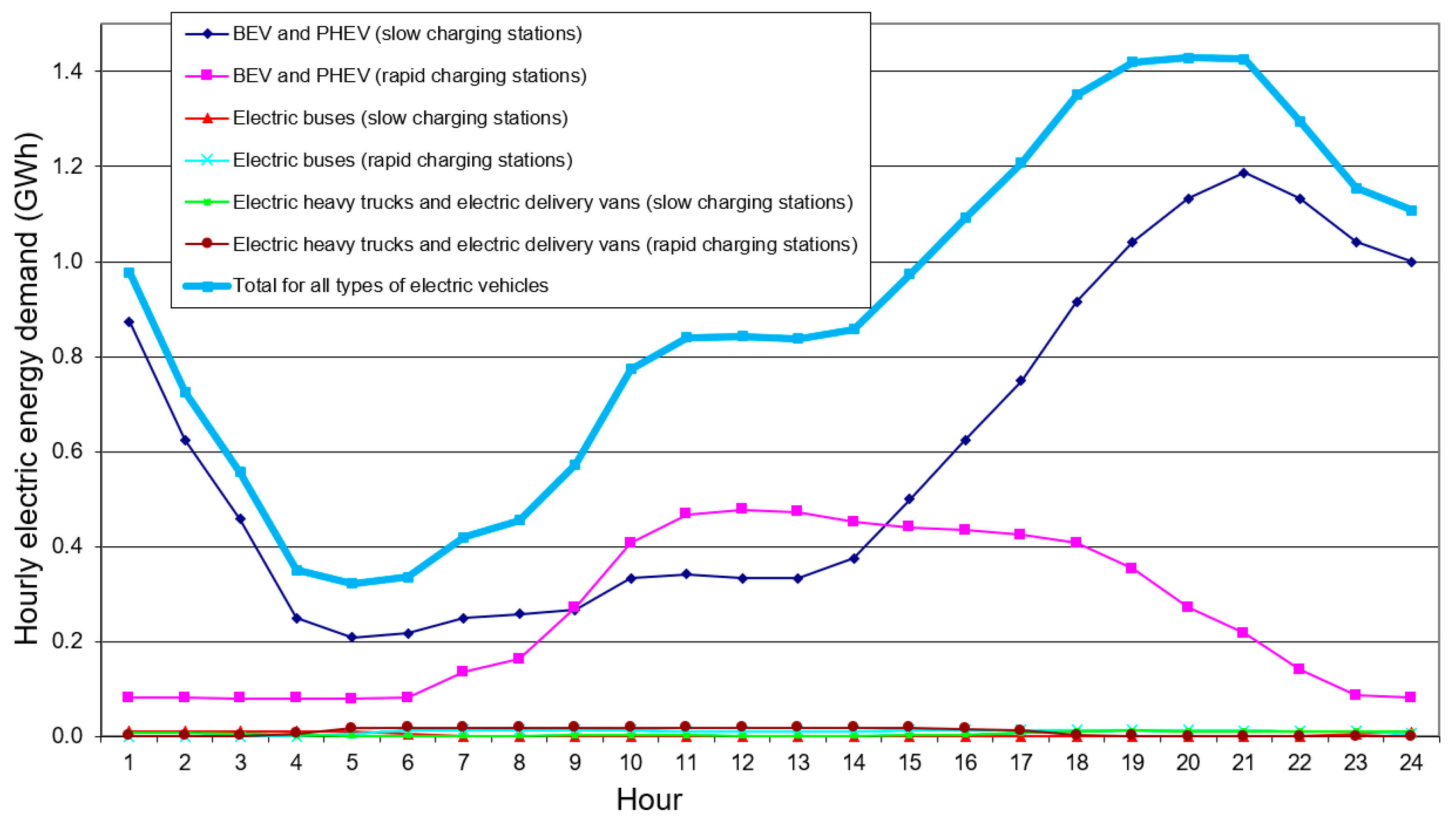
In Step Two, daily profiles of power demand for EV charging were calculated. Calculations of hourly figures from daily profiles of power demand, due solely to e-mobility, used the relative profiles developed for a business day for EVs and daily power demand from four EV categories calculated on annual values. The subsequent calculations assumed that BEVs and PHEVs belonged to a single category, cars with the same relative profiles. The methodology of construction of relative hourly profiles for EV power demand and the relative profiles alone are described in detail in [36]. A total of six relative profiles were used. Each of the three EV categories had two profiles, power drawn from rapid charging stations and from slow charging stations. Slow charging was assumed to be the following: 70% for electric cars, 20% for electric buses and 35% for electric heavy trucks and electric delivery vans, and the remaining power was drawn from rapid charging stations.

Calculations were performed for the three variants of forecast EV numbers in each EV category separately, for 2022–2027. In the next step, combined daily power demand for charging EVs of any type was calculated. Figure 16 shows the outcome of calculations for the balanced variant of the forecast number of EVs in 2027.

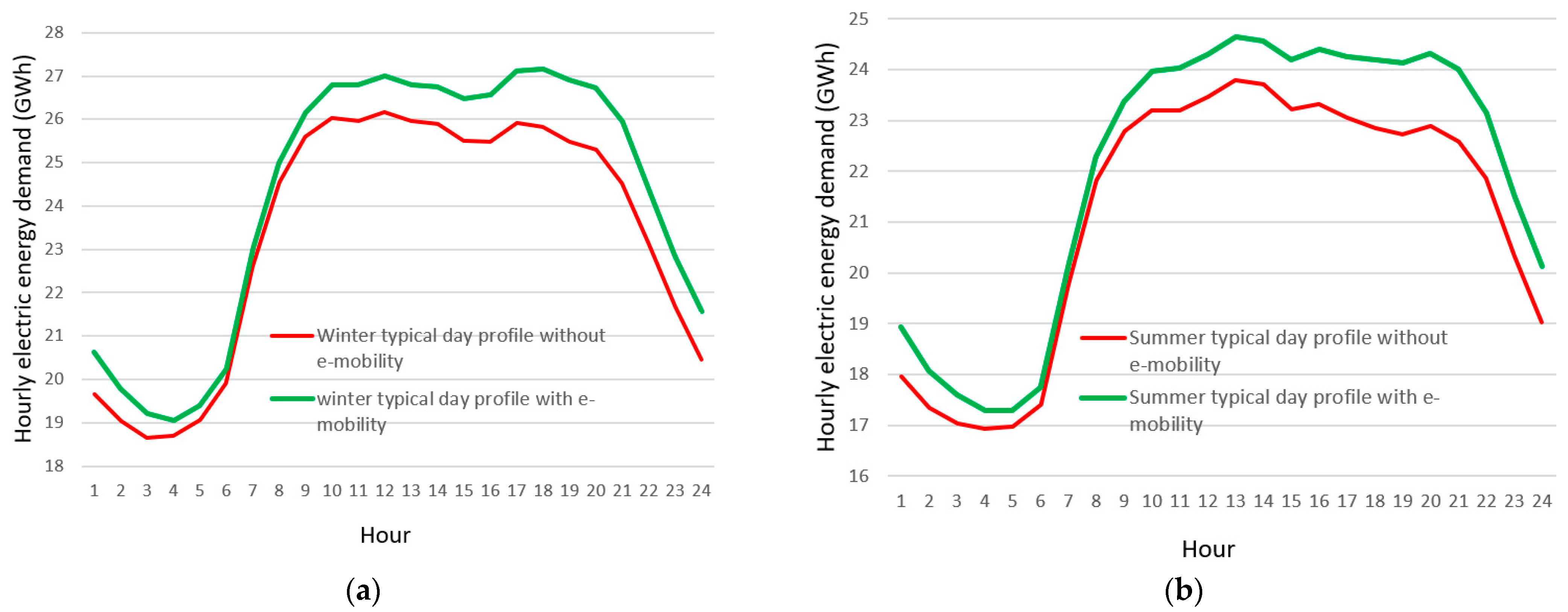
In the third and last step, power demand for the typical winter day profile and typical summer day profile were calculated taking into account the development of e-mobility. Figure 17 presents daily power demand profiles for the typical winter and summer days with and without e-mobility for the balanced variant of the number of EVs in 2027.

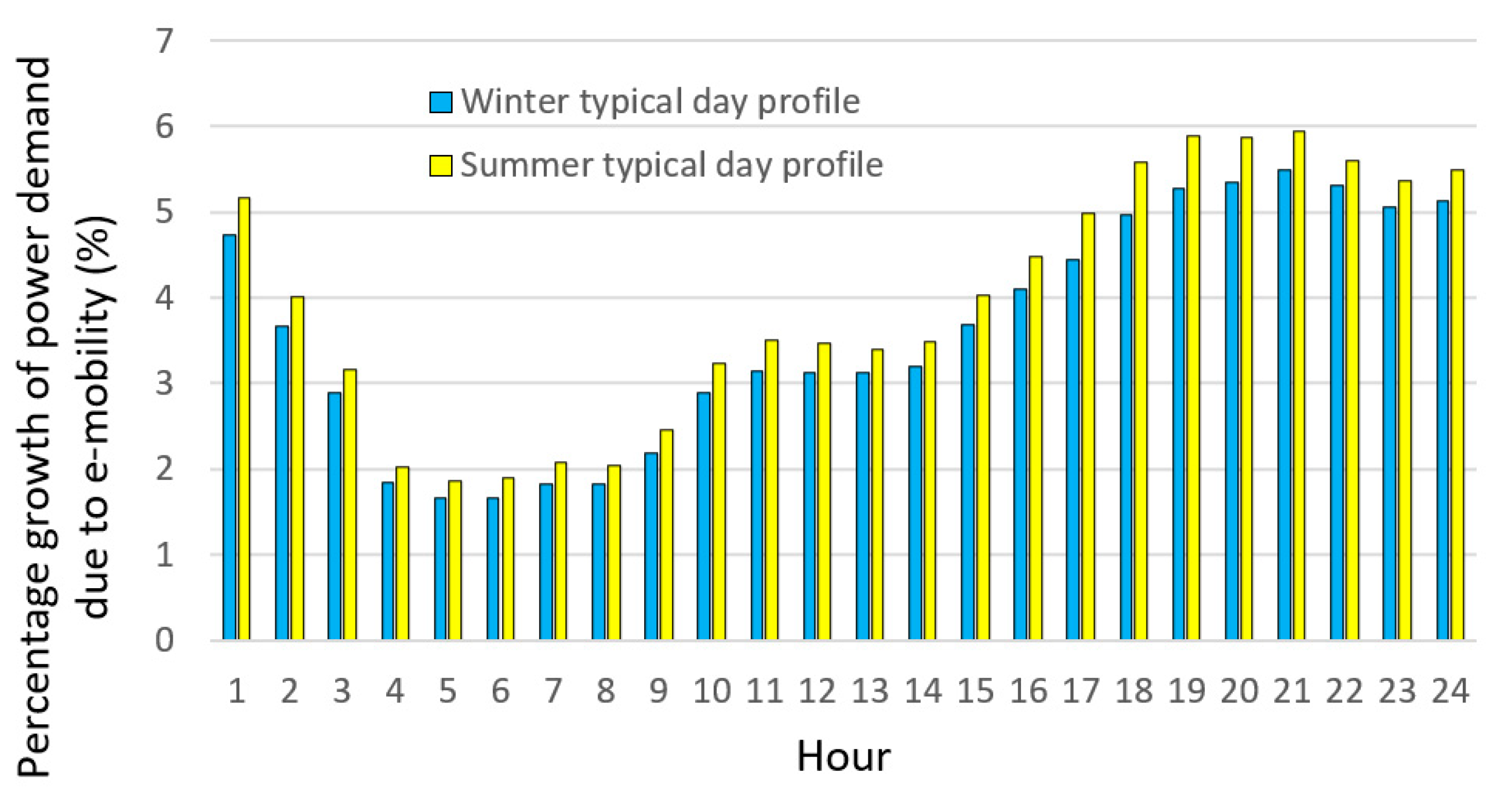
Percentage growth of power demand due to e-mobility for the balanced variant varied by the time of the day. For the typical winter and summer day profiles, the distribution of percentages within a day were very similar. During the “evening” peak, the percentage share of e-mobility was largest, whereas during the night “valley”, the percentage share was the lowest. For the summer typical day profile, percentage shares of e-mobility for all times of the day were slightly higher than for the winter typical day profile. Figure 18 shows the percentage growth of power demand due to e-mobility for the balanced variant of forecast number of EVs in 2027, for the typical winter and summer days. This was due to the fact that, in the winter period, power demand was slightly more than in the summer period, and power demand values due to e-mobility were adopted to be the same for both seasons of the year.

4. Discussion

Our observation is that, for the forecast number of EVs and for the forecast demand for power from the Polish electric power system, the models with the best fit, within the models’ parameter estimation ranges (RMSE metric), generated at the same time the smallest “ex-ante” (forward-looking) forecast values of all methods. The opposite was noted for models with the worst fit to the observed values within the models’ parameter estimation range (RMSE metric). These models, at the same time, generated “ex ante” (forward-looking) forecasts with the highest values of all methods. The conclusion could be, therefore, that well-fitting models would tend to underestimate forecast values, and models with a relatively poor fit would tend to overestimate the forecasts.

Regarding the forecast impact of e-mobility on the Polish electric power system, forecasts (pessimistic variant, balanced variant, and optimistic variant) could be noted to vary more with growing forecast horizon. Particularly wide differences occurred for six years’ advance (2027). Therefore, the conclusion could be that uncertainty of forecasts for that horizon was relatively large. The increase in electric power demand for 2027 in the optimistic variant was almost 7%, which is a significant warning signal as to potential problems with meeting power requirements in Poland.

Our study forecasted on average 0.85 million EVs and 1.54–2.38 TWh corresponding load for the year 2025. Comparatively, previous studies determined the EV number to be 3.64 million and energy to be 6.11 TWh [37] or 0.021–0.176 million EVs and 0.19–1.5 TWh, respectively [25]. For the first study, the number of EVs was quadruple and amount of energy was more than twice to almost quadruple greater than in our forecasts. The difference could be attributed to the first study using a simplified procedure of calculation, not decomposing EVs into categories, and the short period used for forecast parameters estimation. Although the second study decomposed EVs into categories, it also used pre-2019 data. This period concerns time when EVs were treated like a novelty in Poland rather than a valid conventional car alternative. It can be noted that from that period of pioneering EVs in Poland the dynamic of process has changed steeply and EVs have started to be bought on a much larger scale, so more recent data has better accuracy.

Our demand forecasts excluding e-mobility determined that demand in 2025 would equal ca.180 TWh (on different model average). Comparatively, another study forecast 149 TWh with quasi-linear dynamics of growth [7]. We deem the results to be roughly comparable, as flattening of the curve can be attributed to the referred authors using ca. 20 years for training phase of the forecasting model instead of using less, but fresher data, thus obtaining a more conservative, averaged forecast.

The pace of growth in the number of electric trucks, especially heavy ones, is a big unknown. Currently, this segment of e-mobility is in its inception phase, and the momentum of this process is unknown. For electric buses, the growth ceiling, and, therefore, the current impact on the Polish electric power system is quite low, due to the relatively small total number of buses used in Poland (slightly more than 12,000 pcs). Even so, financial inequalities between Polish regions make the future transformation process unequal. Due to the cost of acquisition of vehicles and loading infrastructure one can expect that the biggest cities will note the greatest increase in the number of electric buses. Study concerning the dynamics of growth for the Polish capital city showed tripling of the number of electric buses over 2021–2022, for instance [38]. Although the study referred to determined lack of problems for charging infrastructure with the increase of number of electric buses, the result could potentially vary with region and situation. Current socio-political factors, such as petrol prices or increasing inflation, could also affect interest of customers in using public transport, and, in turn, further increase number of electric buses. Another valid method of eco-transport, especially in big cities, are individual and shared e-scooters. This vehicle type could potentially optimize energy spent per capita for routes without good direct connection by electric buses, and reduce traffic. Facilitating movement of this vehicle requires, however, adoption of proper legislation to ensure safety of drivers, especially in the face of the increasing popularity of this solution [39].

Meanwhile, the potential for rising numbers of electric trucks is very large. Currently there are more than 3.6 million such vehicles registered in Poland. If all of those vehicles became electric, their impact on power demand would be huge. Assuming that the share of electric vans is 75% and of electric heavy trucks 25% out of 3.6 million of electric trucks overall, annual power demand resulting only from electric trucks would be, according to our calculations, about 118,000 TWh, i.e., 33% more than the current (2021) total annual power production in Poland.

The analysis of the results of the forecasts of relative power demand profiles shows that the dynamics of change in both relative profiles decrease significantly over 2022–2027 as compared to changes after 2009. For both relative profiles, the largest changes between 2009 and 2027 (forecast) are visible during the evening “peak” of power demand. In the winter season, the evening “peak” of power demand would have decreased over time, while in the summer period, the evening “peak” of power demand would have increased over time. Since 2009 to about 2016, the dynamics of change in relative profiles was high. In the subsequent years since 2017 and to 2021 the changes became less dynamic, the same applies to forecasts from 2022 to 2027.

Analyses of the impact of e-mobility on the Polish power system until 2027 show that, for the profiles of the typical winter and summer days the percentage share of e-mobility is the highest during the evening “peak”, which is very unfavourable for the electric power system. This could be partially alleviated by changing the habits of EV users so that they begin slow charging of their EVs just after midnight rather than from afternoon (after returning from work). However, this requires incentives for EV users, such as a significantly reduced electricity price at night. To avoid local grid overload, remote control of the charging process seems to be necessary for users charging their vehicles at night. The controller could collaborate with the controllers of other cars, thus, coordinating the charging process in the respective part of the network, and with the power meter, thus, increasing the automation of the process, or by deploying demand management software. Recent studies show, however, that user acceptance of external management of their cars is rather low in Poland [40]. In light of this, more effort should be put into either policy or incentives creation, as solutions such as V2G could decrease the negative impact of increased load caused by electric vehicles [26]. Albeit not all factors influencing the customers are easily transferable between countries, the quality of quick-charging infrastructure and simplicity of use could be named as universal factors impacting users’ decisions to join such programs [27].

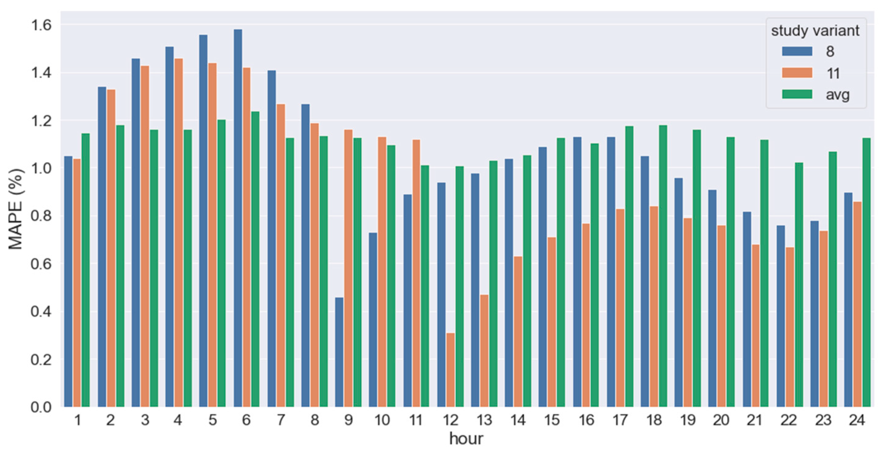
The work on hourly electricity profiles, excluding EV, can be compared with the work of Brodowski et al. [15], where the authors predicted mean hourly load profile in the Polish Electric Grid starting from 11 am in the first variant and 8 am in the second one. In order to compare accuracy of the studies, our summer and wind profiles were averaged over hours, and presented in Figure 19. The comparison determined that both studies resulted in a similar magnitude of error, though the referred study showed higher deviation from average from both sides of the average. For early morning (hourly periods 2–8) our model showed more accuracy, while for the rest of the periods both study models were comparable. It can be noted that 8/11 models demonstrated lowest error directly after moments of start, with rapid increase shortly after. Our model, in turn, was more stable in all analysed periods. It must be, however, emphasised that, due to the difference in tested period ranges (year 2004 for 8/11 models, years 2009–2021 in our model) the above comparison could only be roughly done. Other studies, pertaining to profile creation with decomposition into summer and winter day profiles, resulted in 2.8% MAPE over the year 2016 [18]. In view of the nature of our study, concerning forward extrapolation, both of the above studies cannot be directly compared with our study, as it had no direct test data equivalent.

5. Conclusions

As a result of multi-step and multi-variant forecasts, the impact of e-mobility on the Polish electric power system was determined in terms of annual growth of power demand and on a daily basis (times of the day) for two typical days (summer and winter ones). This impact varied by e-mobility development variant. For the balanced (i.e., the most likely) growth variant, annual power demand would grow by almost 7% due to e-mobility. However, the percentage growth of power demand due to e-mobility for the balanced variant varied by the time of the day. For typical winter and summer day profiles, the distribution of percentages in different times of the day was very similar. During the “evening” peak, the percentage share of e-mobility was the largest, whereas during the night “valley”, the percentage share was the lowest.

The outcomes of forecast power demand amounts in particular times of typical winter and summer days (2022–2027) without e-mobility indicated that, depending on the time of the day, the trends of changes in relative demand were different. For the profile of the typical winter day, relative power demand fell slightly in particular hours between 01:00 pm and midnight between the last year of the forecast (2027) and the first year of the forecast (2022). In the night “valley”, profile changes were minimal.

This research shows that the development of e-mobility in Poland for the horizon of 6 years (2027) may cause a problem regarding covering the additional demand for electricity. The problem concerns both the value of the total annual energy demand, but also the “evening” peak of the typical summer and winter days, in which the impact of e-mobility on the demand for electricity is greatest.

The proposed unique methods developed by the authors proved to be effective. An MLP artificial neural network was applied for non-linear extrapolation of a single function (forecast number of electric vehicles in Poland from 2022 to 2027 and forecast annual power demand in Poland from 2022 to 2027, without the development of e-mobility in Poland). Ensemble Methods (MLP and LSTM) were applied to conduct simultaneous extrapolation of 24 non-linear functions (forecast daily profiles of typical days in 2022–2027 without e-mobility).

A novel, original Growth Dynamics Model was developed that used forecast annual growth ratios to forecast the number of electric vehicles in Poland from 2022 to 2027.

This research has some limitations which should be pointed out in order to ensure the integrity of scientific research. The main limitation is the use of only the time series of forecasted processes in forecasting models. For this reason, the proposed methods of EV number forecasting can be considered appropriate only for the medium-term horizon (up to several years ahead) due to the relatively short time series of historical data and the dependence of the forecasted process on many factors that may undergo dynamic changes in the future (electricity price, incentives supporting e-mobility, dynamic development of hydrogen-powered electric cars, FCV (Fuel Cell Vehicle)). In the case of forecasts of profiles of typical days, for forecast horizons greater than 6 years, one should expect more and more errors in forecasts as the forecast horizon grows. In the future, there may be various additional factors influencing the shape of the typical day profiles. A factor that may affect the shape of the daily load profiles is, for example, the development of RES. Other factors include climate change and the introduction of dynamic tariffs.

We intend to expand future research on e-mobility development to include forecasts of the development of the number of charging stations, discriminating between rapid and slow charging stations, and forecast the development of e-mobility in as disaggregated a manner as possible (separate forecasts by EV type, including electric bikes and scooters). Regarding the research on the impact of e-mobility development on the electric power system, changes in profiles of typical days due to RES development in Poland (wind farms, photovoltaic systems, and energy storage) can be taken into account or studied in addition. An important element planned in future research will be the use of exogenous explanatory variables (input data) in prognostic models (historical values and forecasts), in addition to the withdrawn values of the explained variable.