
The Use of Singular Spectrum Analysis and K-Means Clustering-Based Bootstrap to Improve Multistep Ahead Load Forecasting


Abstract
:1. Introduction
2. Materials and Methods
2.1. Forecasting Methods
2.2. SSA Decomposition Method
2.3. Bagging and Ensemble Methods
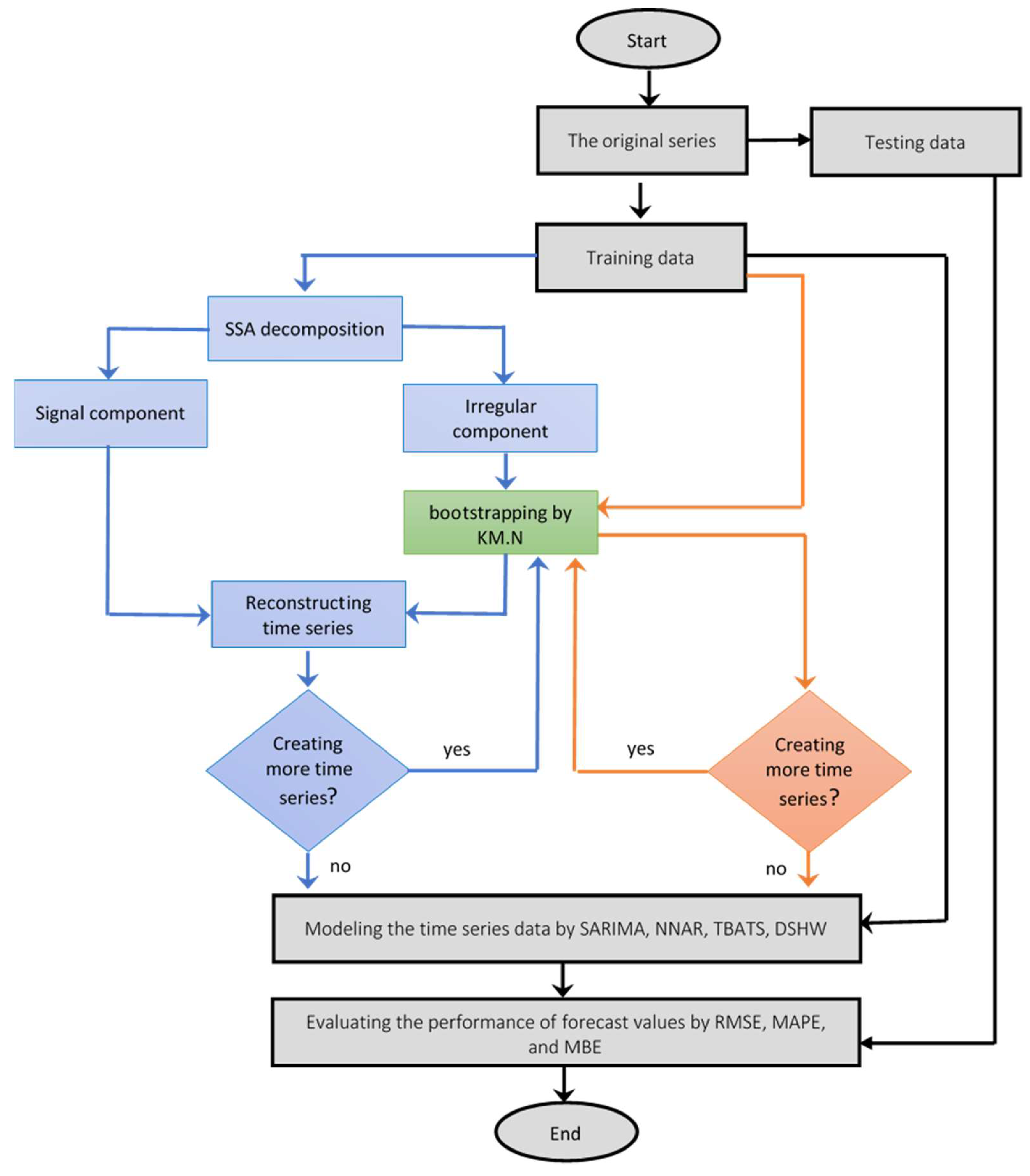
2.4. Proposed Approach
- Step 1.
- Divide the series into the following two parts: training and testing datasets;
- Step 2.
- Generate new series from the original training data by the KM.N method;
- Step 3.
- Generate new series from the original training data by the SSA.KM.N method;
- a.
- Apply SSA to the original training data to define the signal and the irregular component;
- b.
- Generate new series from the irregular component obtained in Step 3a by the KM.N method;
- c.
- Sum each new irregular component obtained from Step 3b with the signal component so that we obtain bootstrapped series of the original training data;
- Step 4.
- Model the original training data, and each bootstrapped series by SARIMA, NNAR, TBATS, and DSHW;
- Step 5.
- Calculate up to M-steps-ahead forecast values by each model obtained in Step 4;
- a.
- Define the M-steps-ahead forecast values from the SARIMA, NNAR, TBATS, and DSHW models obtained from the original training data series;
- b.
- Apply mean and median to calculate the final forecast of the bootstrap series determined in Step 2 and Step 3 for the first bootstrap series;
- Step 6.
- Evaluate the forecast accuracy based on root mean square error (RMSE) and mean absolute percentage error (MAPE).
3. Results and Discussion
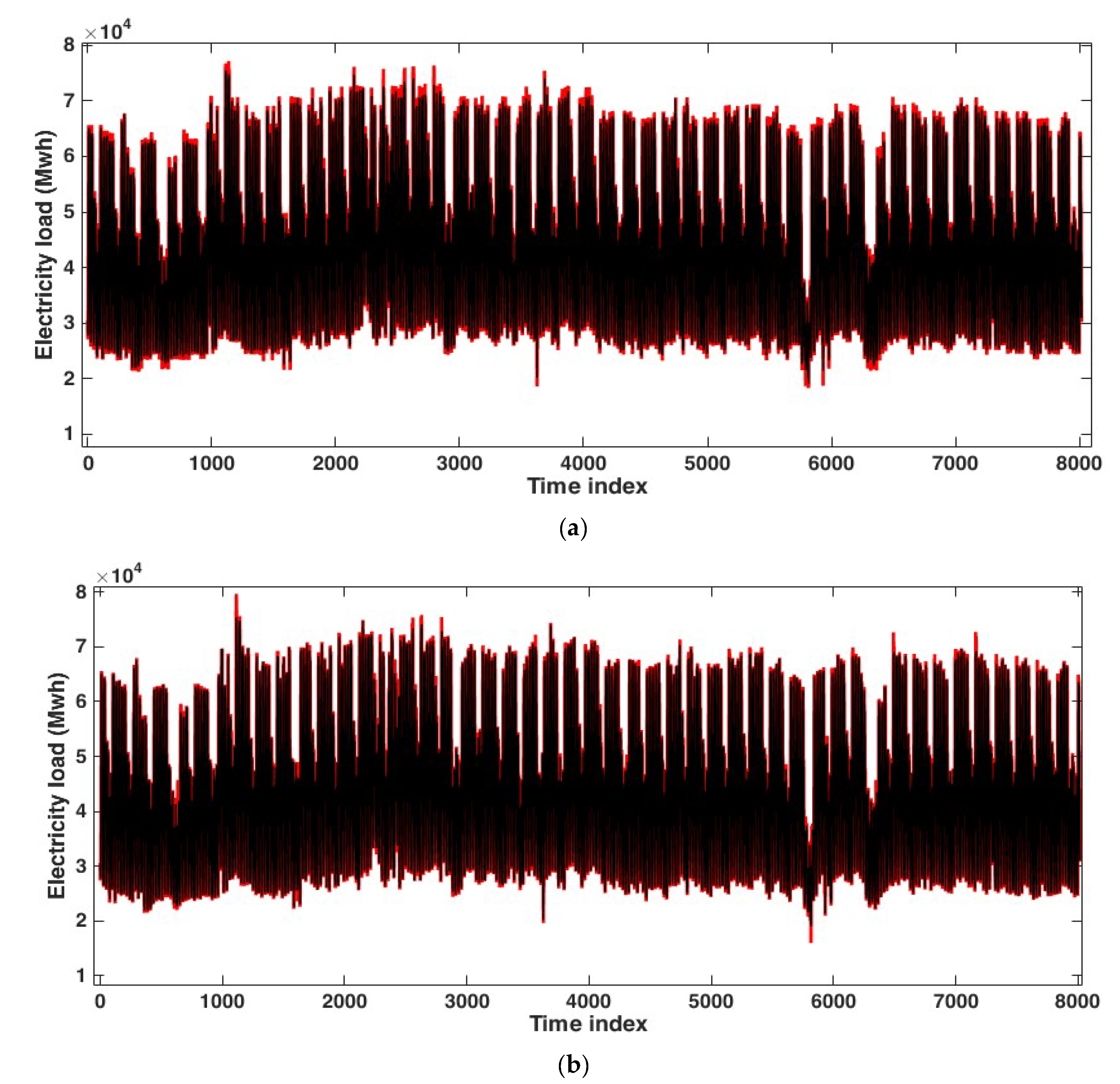
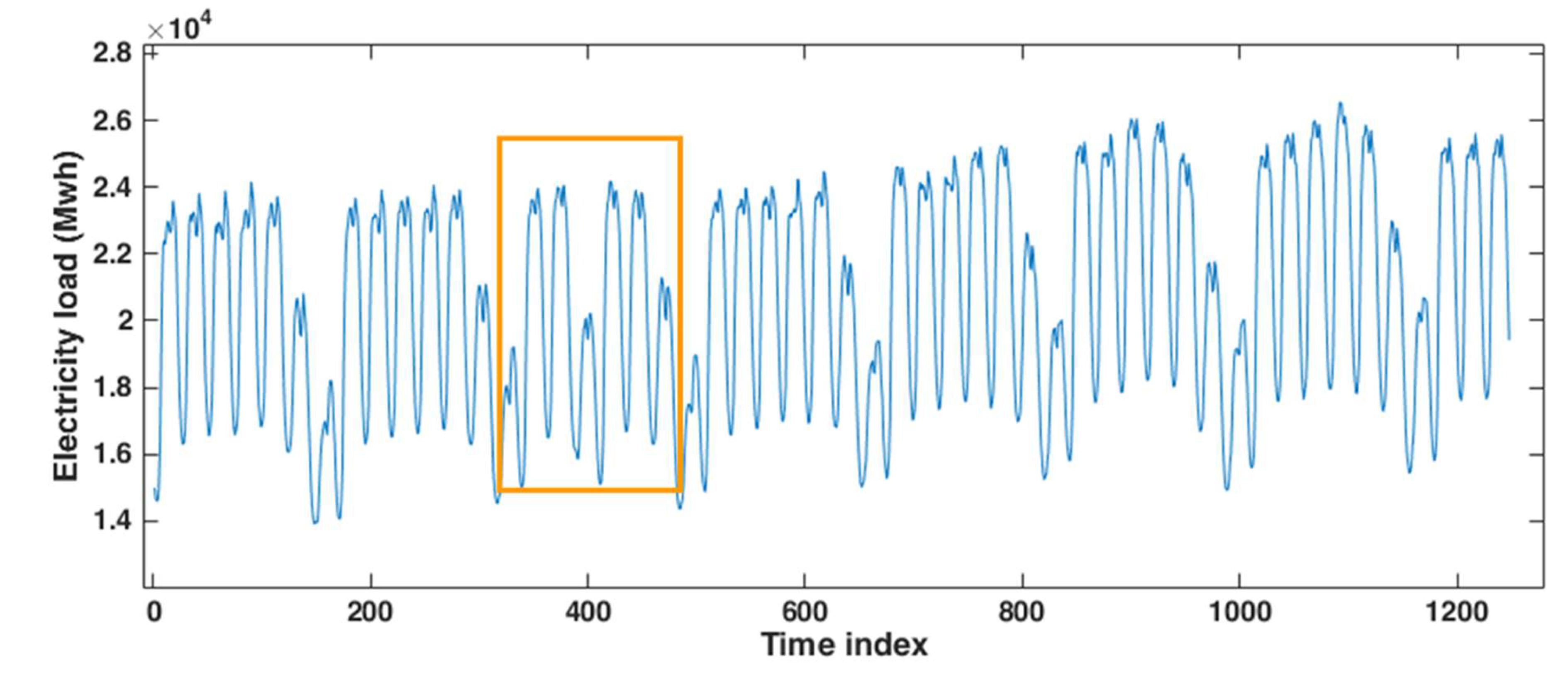
3.1. Application to the Hourly Electricity Load of Johor, Malaysia
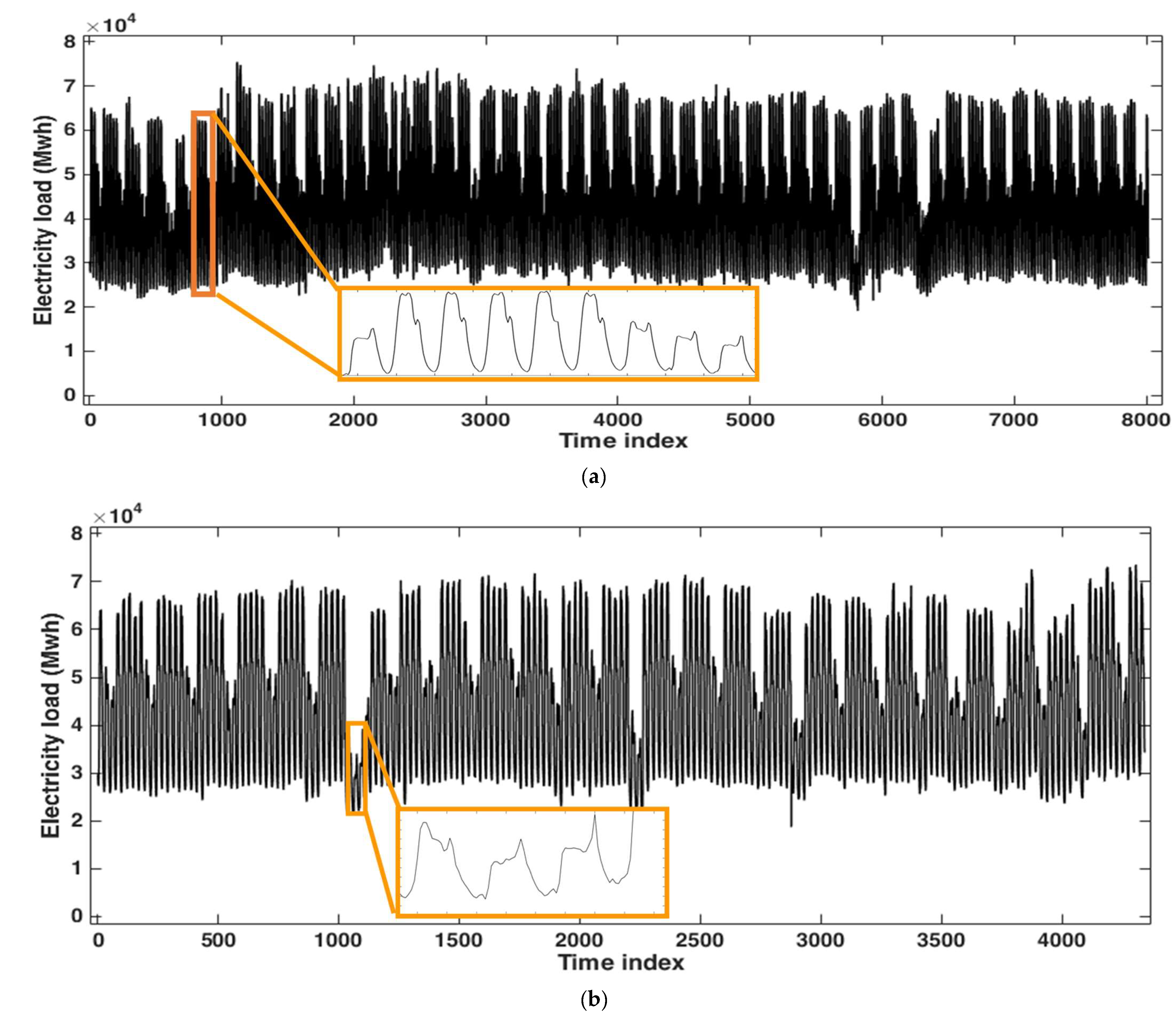
3.2. Application to the Hourly Electricity Load of Poland
3.3. Application to the Hourly Electricity Load of Java-Bali, Indonesia
4. Conclusions
Author Contributions
Funding
Institutional Review Board Statement
Data Availability Statement
Acknowledgments
Conflicts of Interest
Abbreviations
| Abbreviation | Definition |
| DSHW | Double Seasonal Holt-Winters |
| KM | K-means Clustering-Based |
| KM.N | K-means Clustering-Based Generated from Gaussian Normal Distribution |
| MAPE | Mean Absolute Percentage Error |
| MBE | Mean Bias Error |
| MBB | Moving Block Bootstrap |
| NN | Neural Network |
| NNAR | Neural Network Autoregressive |
| RMSE | Root Mean Square Error |
| SARIMA | Seasonal Autoregressive Integrated Moving Average |
| S.MBB | Smoothed Moving Block Bootstrap |
| SSA | Singular Spectrum Analysis |
| SSA.KM.N | Singular Spectrum Analysis, K-means Clustering-Based Generated from Gaussian Normal Distribution |
| STL | Seasonal and Trend decomposition using Loess |
| SVD | Singular Value Decomposition |
| TBATS | Trigonometric, Box–Cox transform, ARMA errors, Trend, and Seasonal Components |
References
- Ahmad, W.; Ayub, N.; Ali, T.; Irfan, M.; Awais, M.; Shiraz, M.; Glowacz, A. Towards Short Term Electricity Load Forecasting Using Improved Support Vector Machine and Extreme Learning Machine. Energies 2020, 13, 2907. [Google Scholar] [CrossRef]
- Ayub, N.; Irfan, M.; Awais, M.; Ali, U.; Ali, T.; Hamdi, M.; Alghamdi, A.; Muhammad, F. Big Data Analytics for Short and Medium-Term Electricity Load Forecasting Using an AI Techniques Ensembler. Energies 2020, 13, 5193. [Google Scholar] [CrossRef]
- De Livera, A.M.; Hyndman, R.J.; Snyder, R.D. Forecasting Time Series with Complex Seasonal Patterns Using Exponential Smoothing. J. Am. Stat. Assoc. 2011, 106, 1513–1527. [Google Scholar] [CrossRef]
- Soares, L.J.; Medeiros, M.C. Modeling and Forecasting Short-Term Electricity Load: A Comparison of Methods with an Ap-plication to Brazilian Data. Int. J. Forecast. 2008, 24, 630–644. [Google Scholar] [CrossRef]
- Sulandari, W.; Subanar, S.; Suhartono, S.; Utami, H.; Lee, M.H.; Rodrigues, P.C. SSA-Based Hybrid Forecasting Models and Applications. Bull. Electr. Eng. Inform. 2020, 9, 2178–2188. [Google Scholar] [CrossRef]
- Bernardi, M.; Petrella, L. Multiple Seasonal Cycles Forecasting Model: The Italian Electricity Demand. Stat. Methods Appl. 2015, 24, 671–695. [Google Scholar] [CrossRef]
- López, M.; Valero, S.; Sans, C.; Senabre, C. Use of Available Daylight to Improve Short-Term Load Forecasting Accuracy. Energies 2021, 14, 95. [Google Scholar] [CrossRef]
- Hong, T.; Wang, P.; White, L. Weather Station Selection for Electric Load Forecasting. Int. J. Forecast. 2015, 31, 286–295. [Google Scholar] [CrossRef]
- Luo, J.; Hong, T.; Fang, S.-C. Benchmarking Robustness of Load Forecasting Models under Data Integrity Attacks. Int. J. Forecast. 2018, 34, 89–104. [Google Scholar] [CrossRef]
- Sadaei, H.J.; de Lima e Silva, P.C.; Guimarães, F.G.; Lee, M.H. Short-Term Load Forecasting by Using a Combined Method of Convolutional Neural Networks and Fuzzy Time Series. Energy 2019, 175, 365–377. [Google Scholar] [CrossRef]
- Cabrera, N.G.; Gutiérrez-Alcaraz, G.; Gil, E. Load Forecasting Assessment Using SARIMA Model and Fuzzy Inductive Rea-soning. In Proceedings of the 2013 IEEE International Conference on Industrial Engineering and Engineering Management, Bangkok, Thailand, 10–13 December 2013; pp. 561–565. [Google Scholar] [CrossRef]
- Chikobvu, D.; Sigauke, C. Regression-SARIMA Modelling of Daily Peak Electricity Demand in South Africa. J. Energy South. Afr. 2012, 23, 23–30. [Google Scholar] [CrossRef]
- Taylor, J.W. Short-Term Electricity Demand Forecasting Using Double Seasonal Exponential Smoothing. J. Opera. Tional. Res. Soc. 2003, 54, 799–805. [Google Scholar] [CrossRef]
- Taylor, J.W. Triple Seasonal Methods for Short-Term Electricity Demand Forecasting. Eur. J. Oper. Res. 2010, 204, 139–152. [Google Scholar] [CrossRef]
- Arora, S.; Taylor, J.W. Short-Term Forecasting of Anomalous Load Using Rule-Based Triple Seasonal Methods. IEEE Trans. Power Syst. 2013, 28, 3235–3242. [Google Scholar] [CrossRef]
- Bakirtzis, A.G.; Petridis, V.; Kiartzis, S.J.; Alexiadis, M.C.; Maissis, A.H. A Neural Network Short Term Load Forecasting Model for the Greek Power System. IEEE Trans. Power Syst. 1996, 11, 858–863. [Google Scholar] [CrossRef]
- Charytoniuk, W.; Chen, M.-S. Very Short-Term Load Forecasting Using Artificial Neural Networks. IEEE Trans. Power Syst. 2000, 15, 263–268. [Google Scholar] [CrossRef]
- Mordjaoui, M.; Haddad, S.; Medoued, A.; Laouafi, A. Electric Load Forecasting by Using Dynamic Neural Network. Int. J. Hydrogen Energy 2017, 42, 17655–17663. [Google Scholar] [CrossRef]
- Leite Coelho da Silva, F.; da Costa, K.; Canas Rodrigues, P.; Salas, R.; López-Gonzales, J.L. Statistical and Artificial Neural Networks Models for Electricity Consumption Forecasting in the Brazilian Industrial Sector. Energies 2022, 15, 588. [Google Scholar] [CrossRef]
- Sulandari, W.; Subanar, S.; Suhartono, S.; Utami, H. Forecasting Time Series with Trend and Seasonal Patterns Based on SSA. In Proceedings of the 2017 3rd International Conference on Science in Information Technology (ICSITech) Theory and Applicattion of IT for Education, Industry and Society in Big Data Era, Bandung, Indonesia, 25–26 October 2017; pp. 694–699. [Google Scholar] [CrossRef]
- Zhang, X.; Wang, J.; Zhang, K. Short-Term Electric Load Forecasting Based on Singular Spectrum Analysis and Support Vector Machine Optimized by Cuckoo Search Algorithm. Electr. Power Syst. Res. 2017, 146, 270–285. [Google Scholar] [CrossRef]
- Sulandari, W.; Subanar, S.; Lee, M.H.; Rodrigues, P.C. Time Series Forecasting Using Singular Spectrum Analysis, Fuzzy Systems and Neural Networks. MethodsX 2020, 7, 101015. [Google Scholar] [CrossRef]
- Tao, D.; Xiuli, W.; Xifan, W. A Combined Model of Wavelet and Neural Network for Short Term Load Forecasting. In Proceedings of the International Conference on Power System Technology, Kunming, China, 13–17 October 2002; Volume 4, pp. 2331–2335. [Google Scholar] [CrossRef]
- Moazzami, M.; Khodabakhshian, A.; Hooshmand, R. A New Hybrid Day-Ahead Peak Load Forecasting Method for Iran’s National Grid. Appl. Energy 2013, 101, 489–501. [Google Scholar] [CrossRef]
- Pandian, S.C.; Duraiswamy, K.; Rajan, C.C.A.; Kanagaraj, N. Fuzzy Approach for Short Term Load Forecasting. Electr. Power Syst. Res. 2006, 76, 541–548. [Google Scholar] [CrossRef]
- Al-Kandari, A.M.; Soliman, S.A.; El-Hawary, M.E. Fuzzy Short-Term Electric Load Forecasting. Int. J. Electr. Trical. Power Energy Syst. 2004, 26, 111–122. [Google Scholar] [CrossRef]
- Chen, Y.; Yang, Y.; Liu, C.; Li, C.; Li, L. A Hybrid Application Algorithm Based on the Support Vector Machine and Artificial Intelligence: An Example of Electric Load Forecasting. Appl. Math. Model. 2015, 39, 2617–2632. [Google Scholar] [CrossRef]
- Li, Y.; Fang, T.; Yu, E. Study of Support Vector Machines for Short-Term Load Forecasting. Proc. CSEE 2003, 23, 55–59. [Google Scholar]
- Breiman, L. Bagging Predictors | SpringerLink. Mach. Learn. 1996, 24, 123–140. [Google Scholar] [CrossRef]
- Bergmeir, C.; Hyndman, R.J.; Benítez, J.M. Bagging Exponential Smoothing Methods Using STL Decomposition and Box–Cox Transformation. Int. J. Forecast. 2016, 32, 303–312. [Google Scholar] [CrossRef]
- Petropoulos, F.; Hyndman, R.J.; Bergmeir, C. Exploring the Sources of Uncertainty: Why Does Bagging for Time Series Fore-casting Work? Eur. J. Oper. Res. 2018, 268, 545–554. [Google Scholar] [CrossRef]
- Laurinec, P.; Lóderer, M.; Lucká, M.; Rozinajová, V. Density-Based Unsupervised Ensemble Learning Methods for Time Series Forecasting of Aggregated or Clustered Electricity Consumption. J. Intell. Inf. Syst. 2019, 53, 219–239. [Google Scholar] [CrossRef]
- Cleveland, R.B.; Cleveland, W.S.; Terpenning, I. STL: A Seasonal-Trend Decomposition Procedure Based on Loess. J. Off. Stat. 1990, 6, 3. [Google Scholar]
- Box, G.E.; Jenkins, G.M.; Reinsel, G.C.; Ljung, G.M. Time Series Analysis: Forecasting and Control; John Wiley & Sons: Hoboken, NJ, USA, 2015. [Google Scholar]
- Wei, W.W.-S. Time Series Analysis: Univariate and Multivariate Methods, 2nd ed.; Pearson Addison-Wesley: Boston, MA, USA, 2006. [Google Scholar]
- Huang, S.-J.; Shih, K.-R. Short-Term Load Forecasting via ARMA Model Identification Including Non-Gaussian Process Con-siderations. IEEE Trans. Power Syst. 2003, 18, 673–679. [Google Scholar] [CrossRef]
- Hyndman, R.J.; Khandakar, Y. Automatic Time Series Forecasting: The Forecast Package for R. JSS 2008, 27, 1–23. [Google Scholar] [CrossRef]
- Mohamed, N.; Ahmad, M.H.; Ismail, Z. Improving Short Term Load Forecasting Using Double Seasonal Arima Model. World Appl. Sci. J. 2011, 15, 223–231. [Google Scholar]
- Hyndman, R.J.; Athanasopoulos, G.; Bergmeir, C.; Caceres, G.; Chhay, L.; O’Hara-Wild, M.; Petropoulos, F.; Razbash, S.; Wang, E.; Yasmeen, F. Forecast: Forecasting Functions for Time Series and Linear Models. In R Package Version 8.15. 2021. Available online: https://pkg.robjhyndman.com/forecast/ (accessed on 18 December 2021).
- Hyndman, R.J.; Athanasopoulos, G. Forecasting: Principles and Practice, 2nd ed.; OTexts: Melbourne, Australia, 2018. [Google Scholar]
- Zhang, G.; Patuwo, B.E.; Hu, M.Y. Forecasting with Artificial Neural Networks: The State of the Art. Int. J. Forecast. 1998, 14, 35–62. [Google Scholar] [CrossRef]
- Sulandari, W.; Suhartono; Subanar; Rodrigues, P.C. Exponential Smoothing on Modeling and Forecasting Multiple Seasonal Time Series: An Overview. Fluct. Noise Lett. 2021, 20, 2130003. [Google Scholar] [CrossRef]
- Sulandari, W.; Subanar, S.; Suhartono, S.; Utami, H. Forecasting Electricity Load Demand Using Hybrid Exponential Smoothing-Artificial Neural Network Model. Int. J. Adv. Intell. Inform. 2016, 2, 131–139. [Google Scholar] [CrossRef]
- Hyndman, R.; Koehler, A.B.; Ord, J.K.; Snyder, R.D. Forecasting with Exponential Smoothing: The State Space Approach; Springer Science & Business Media: Berlin, Germany, 2008. [Google Scholar]
- Golyandina, N.; Osipov, E. The “Caterpillar”-SSA Method for Analysis of Time Series with Missing Values. J. Stat. Plan. Inference 2007, 137, 2642–2653. [Google Scholar] [CrossRef]
- Golyandina, N.; Korobeynikov, A. Basic Singular Spectrum Analysis and Forecasting with R. Comput. Stat. Data Anal. 2014, 71, 934–954. [Google Scholar] [CrossRef]
- Golyandina, N.; Zhigljavsky, A. Singular Spectrum Analysis for Time Series, 2nd ed.; Springer Briefs in Statistics; Springer: Berlin/Heidelberg, Germany, 2020. [Google Scholar] [CrossRef]
- Golyandina, N.; Korobeynikov, A.; Zhigljavsky, A. Singular Spectrum Analysis with R; Springer: Berlin, Germany, 2018. [Google Scholar]
- PetoLau/petolau.github.io. GitHub. Available online: https://github.com/PetoLau/petolau.github.io (accessed on 19 April 2021).
- Hassani, H. Singular Spectrum Analysis: Methodology and Comparison. J. Data Sci. 2007, 5, 239–257. [Google Scholar] [CrossRef]
- Hyndman, R.J.; Koehler, A.B. Another Look at Measures of Forecast Accuracy. Int. J. Forecast. 2006, 22, 679–688. [Google Scholar] [CrossRef]
- Stone, R.J. Improved Statistical Procedure for the Evaluation of Solar Radiation Estimation Models. Sol. Energy 1993, 51, 289–291. [Google Scholar] [CrossRef]
- Guimaraes, F.; Javedani Sadaei, H. Data for: Short-Term Load Forecasting by Using a Combined Method of Convolutional Neural Networks and Fuzzy Time Series. Mendeley Data 2019, Version 1. Available online: https://data.mendeley.com/datasets/f4fcrh4tn9/1 (accessed on 5 March 2021).
- Sulandari, W.; Subanar; Lee, M.H.; Rodrigues, P.C. Indonesian Electricity Load Forecasting Using Singular Spectrum Analysis, Fuzzy Systems and Neural Networks. Energy 2020, 190, 116408. [Google Scholar] [CrossRef]
- Montero-Manso, P.; Athanasopoulos, G.; Hyndman, R.J.; Talagala, T.S. FFORMA: Feature-Based Forecast Model Averaging. Int. J. Forecast. 2020, 36, 86–92. [Google Scholar] [CrossRef]
- Smyl, S. A Hybrid Method of Exponential Smoothing and Recurrent Neural Networks for Time Series Forecasting. Int. J. Forecast. 2020, 36, 75–85. [Google Scholar] [CrossRef]


| 1st Data Set | 2nd Data Set | |
|---|---|---|
| Training | 01/01/2009 00:00–30/11/2009 23:00 | 01/01/2010 00:00–30/06/2010 23:00 |
| Testing (for up to h-step ahead): | ||
| = 1 | 01/12/2009 00:00–31/12/2009 23:00 | 01/07/2010 00:00–31/07/2010 23:00 |
| = 12 | 01/12/2009 00:00–01/12/2009 11:00 | 01/07/2010 00:00–01/07/2020 11:00 |
| = 24 | 01/12/2009 00:00–01/12/2009 23:00 | 01/07/2010 00:00–01/07/2020 23:00 |
| = 36 | 01/12/2009 00:00–01/12/2009 11:00 | 01/07/2010 00:00–02/07/2020 11:00 |
| Method | Testing of 1st Data Set (1–31 December 2009) | Testing of 2nd Data Set (1–31 July 2010) | ||
|---|---|---|---|---|
| RMSE | MAPE | RMSE | MAPE | |
| SARIMA | 1168.02 | 1.90 | 1719.68 | 2.54 |
| NNAR | 749.92 | 1.21 | 1182.68 | 1.75 |
| TBATS | 1584.47 | 2.91 | 1466.33 | 2.37 |
| DSHW | 839.18 | 1.29 | 1035.14 | 1.46 |
| 1st Data Set | 2nd Data Set | |||||||||||
|---|---|---|---|---|---|---|---|---|---|---|---|---|
| RMSE | MAPE | RMSE | MAPE | |||||||||
| 12 | 24 | 36 | 12 | 24 | 36 | 12 | 24 | 36 | 12 | 24 | 36 | |
| original | 466.51 | 1408.20 | 2118.07 | 0.88 | 1.94 | 3.13 | 1139.08 | 1268.58 | 1324.19 | 2.27 | 2.48 | 2.97 |
| Bagging + Mean | ||||||||||||
| KM.N | ||||||||||||
| = 25 | 512.57 | 1404.68 | 2035.79 | 0.97 | 1.94 | 3.00 | 1345.29 | 1405.54 | 1366.41 | 2.25 | 2.57 | 2.87 |
| = 50 | 530.99 | 1419.45 | 2049.64 | 0.99 | 1.96 | 3.03 | 1320.97 | 1393.69 | 1366.42 | 2.28 | 2.59 | 2.91 |
| = 75 | 544.23 | 1429.02 | 2053.97 | 1.02 | 1.99 | 3.05 | 1323.97 | 1394.82 | 1367.79 | 2.29 | 2.60 | 2.92 |
| = 100 | 556.73 | 1438.17 | 2062.04 | 1.09 | 2.03 | 3.08 | 1329.88 | 1397.27 | 1371.85 | 2.32 | 2.61 | 2.93 |
| SSA. KM.N | ||||||||||||
| = 25 | 490.52 | 1368.94 | 2029.14 | 1.04 | 1.94 | 2.96 | 1067.12 | 1234.85 | 1286.55 | 2.11 | 2.40 | 2.87 |
| = 50 | 494.71 | 1357.47 | 2018.93 | 1.05 | 1.94 | 2.95 | 1069.56 | 1235.92 | 1288.94 | 2.13 | 2.41 | 2.88 |
| = 75 | 498.23 | 1356.26 | 2015.31 | 1.07 | 1.94 | 2.95 | 1068.79 | 1235.36 | 1288.80 | 2.13 | 2.41 | 2.88 |
| = 100 | 495.76 | 1360.24 | 2018.48 | 1.06 | 1.95 | 2.95 | 1072.37 | 1236.66 | 1289.22 | 2.14 | 2.41 | 2.88 |
| Bagging + Median | ||||||||||||
| KM.N | ||||||||||||
| = 25 | 548.32 | 1415.38 | 2045.61 | 1.03 | 1.98 | 3.04 | 1330.61 | 1388.67 | 1348.25 | 2.12 | 2.49 | 2.80 |
| = 50 | 543.85 | 1424.97 | 2055.74 | 1.02 | 1.98 | 3.05 | 1306.42 | 1383.85 | 1355.37 | 2.18 | 2.53 | 2.86 |
| = 75 | 549.99 | 1430.50 | 2056.88 | 1.05 | 2.00 | 3.06 | 1322.84 | 1390.97 | 1360.40 | 2.22 | 2.55 | 2.88 |
| = 100 | 566.06 | 1444.64 | 2066.11 | 1.09 | 2.04 | 3.09 | 1325.92 | 1392.35 | 1365.12 | 2.27 | 2.58 | 2.90 |
| SSA.KM.N | ||||||||||||
| = 25 | 501.40 | 1372.29 | 2029.04 | 1.10 | 1.98 | 2.98 | 1072.91 | 1239.46 | 1290.89 | 2.13 | 2.41 | 2.88 |
| = 50 | 514.83 | 1355.26 | 2012.78 | 1.13 | 1.97 | 2.95 | 1076.47 | 1239.43 | 1292.00 | 2.15 | 2.42 | 2.89 |
| = 75 | 514.08 | 1355.95 | 2011.37 | 1.13 | 1.97 | 2.95 | 1069.09 | 1234.93 | 1289.34 | 2.13 | 2.41 | 2.88 |
| = 100 | 508.08 | 1365.38 | 2018.37 | 1.11 | 1.97 | 2.96 | 1074.03 | 1238.00 | 1290.43 | 2.15 | 2.42 | 2.88 |
| 1st Data Set | 2nd Data Set | |||||||||||
|---|---|---|---|---|---|---|---|---|---|---|---|---|
| RMSE | MAPE | RMSE | MAPE | |||||||||
| 12 | 24 | 36 | 12 | 24 | 36 | 12 | 24 | 36 | 12 | 24 | 36 | |
| Original | 1761.72 | 2365.26 | 4393.21 | 2.12 | 3.18 | 5.81 | 2474.07 | 2797.86 | 5179.86 | 3.62 | 4.24 | 6.15 |
| Bagging + Mean | ||||||||||||
| KM.N | ||||||||||||
| = 25 | 960.09 | 1723.56 | 2881.12 | 1.10 | 2.35 | 4.01 | 2367.77 | 2062.45 | 4128.65 | 3.50 | 3.32 | 5.19 |
| = 50 | 964.93 | 1730.89 | 2894.54 | 1.12 | 2.37 | 4.03 | 2433.15 | 2096.23 | 4154.82 | 3.58 | 3.34 | 5.22 |
| = 75 | 996.61 | 1747.33 | 2949.97 | 1.16 | 2.39 | 4.08 | 2358.62 | 2044.60 | 4084.19 | 3.48 | 3.28 | 5.13 |
| = 100 | 1007.27 | 1766.48 | 2972.19 | 1.16 | 2.42 | 4.12 | 2388.40 | 2067.72 | 4120.69 | 3.51 | 3.30 | 5.17 |
| SSA. KM.N | ||||||||||||
| = 25 | 973.69 | 1661.79 | 2756.24 | 1.11 | 2.29 | 3.93 | 2279.29 | 1958.57 | 5344.05 | 3.41 | 3.15 | 6.04 |
| = 50 | 954.97 | 1618.73 | 2701.08 | 1.11 | 2.23 | 3.84 | 2349.54 | 1997.22 | 5451.24 | 3.52 | 3.18 | 6.14 |
| = 75 | 971.00 | 1634.74 | 2732.76 | 1.11 | 2.24 | 3.86 | 2325.34 | 1980.90 | 5443.80 | 3.47 | 3.16 | 6.13 |
| = 100 | 968.26 | 1628.32 | 2716.57 | 1.11 | 2.24 | 3.85 | 2311.58 | 1974.44 | 5452.81 | 3.45 | 3.16 | 6.13 |
| Bagging + Median | ||||||||||||
| KM.N | ||||||||||||
| = 25 | 913.18 | 1695.23 | 2836.71 | 1.07 | 2.34 | 3.96 | 2364.00 | 2069.78 | 4029.04 | 3.52 | 3.35 | 5.14 |
| = 50 | 912.72 | 1690.94 | 2861.26 | 1.05 | 2.32 | 3.98 | 2469.39 | 2110.04 | 4136.53 | 3.63 | 3.36 | 5.21 |
| = 75 | 948.08 | 1697.71 | 2883.83 | 1.13 | 2.35 | 4.01 | 2399.13 | 2068.57 | 4035.98 | 3.53 | 3.31 | 5.11 |
| = 100 | 964.86 | 1713.66 | 2892.47 | 1.12 | 2.36 | 4.02 | 2418.19 | 2080.95 | 4088.09 | 3.55 | 3.32 | 5.15 |
| SSA.KM.N | ||||||||||||
| = 25 | 978.42 | 1654.41 | 2785.53 | 1.13 | 2.28 | 3.95 | 2248.30 | 1952.46 | 5361.38 | 3.37 | 3.14 | 6.05 |
| = 50 | 979.69 | 1633.47 | 2657.16 | 1.13 | 2.26 | 3.81 | 2270.89 | 1954.88 | 5411.12 | 3.39 | 3.14 | 6.09 |
| = 75 | 975.65 | 1642.36 | 2683.66 | 1.12 | 2.26 | 3.83 | 2315.22 | 1980.65 | 5475.96 | 3.44 | 3.16 | 6.15 |
| = 100 | 959.00 | 1612.46 | 2631.46 | 1.13 | 2.23 | 3.78 | 2307.14 | 1977.87 | 5438.96 | 3.43 | 3.15 | 6.12 |
| 1st Data Set | 2nd Data Set | |||||||||||
|---|---|---|---|---|---|---|---|---|---|---|---|---|
| RMSE | MAPE | RMSE | MAPE | |||||||||
| 12 | 24 | 36 | 12 | 24 | 36 | 12 | 24 | 36 | 12 | 24 | 36 | |
| original | 1613.36 | 2057.21 | 2146.92 | 4.03 | 3.72 | 4.08 | 1574.78 | 2771.37 | 2685.71 | 3.87 | 5.54 | 5.54 |
| Bagging + Mean | ||||||||||||
| KM.N | ||||||||||||
| = 25 | 1740.64 | 2333.25 | 2360.33 | 3.99 | 3.98 | 3.91 | 1410.82 | 3122.42 | 2864.93 | 3.50 | 5.93 | 5.86 |
| = 50 | 1668.46 | 2245.73 | 2282.53 | 3.89 | 3.86 | 3.84 | 1296.39 | 3045.17 | 2805.20 | 3.18 | 5.67 | 5.63 |
| = 75 | 1664.15 | 2246.18 | 2290.12 | 3.86 | 3.85 | 3.84 | 1280.05 | 3047.59 | 2806.13 | 3.14 | 5.67 | 5.62 |
| = 100 | 1732.41 | 2325.22 | 2370.24 | 3.91 | 3.93 | 3.90 | 1255.27 | 3002.58 | 2775.60 | 3.10 | 5.59 | 5.55 |
| SSA. KM.N | ||||||||||||
| = 25 | 1966.14 | 2547.93 | 2560.87 | 4.61 | 4.44 | 4.26 | 1371.73 | 1974.32 | 2286.35 | 3.43 | 4.03 | 4.61 |
| = 50 | 2023.97 | 2609.35 | 2634.36 | 4.60 | 4.48 | 4.28 | 1447.05 | 1939.14 | 2316.25 | 3.51 | 3.99 | 4.68 |
| = 75 | 2011.41 | 2580.08 | 2615.16 | 4.60 | 4.45 | 4.28 | 1503.40 | 1861.19 | 2247.76 | 3.56 | 3.87 | 4.61 |
| = 100 | 1994.50 | 2572.82 | 2597.21 | 4.59 | 4.45 | 4.27 | 1468.42 | 1879.36 | 2259.16 | 3.52 | 3.90 | 4.60 |
| Bagging + Median | ||||||||||||
| KM.N | ||||||||||||
| = 25 | 1937.56 | 2611.75 | 2574.41 | 4.19 | 4.27 | 4.16 | 1336.97 | 3256.25 | 2953.00 | 3.30 | 6.03 | 5.91 |
| = 50 | 1719.88 | 2336.30 | 2337.81 | 3.86 | 3.90 | 3.87 | 1297.49 | 3240.04 | 2933.74 | 3.19 | 5.96 | 5.83 |
| = 75 | 1818.78 | 2406.98 | 2410.71 | 4.01 | 4.03 | 4.00 | 1297.06 | 3239.03 | 2934.09 | 3.19 | 5.96 | 5.83 |
| = 100 | 2010.25 | 2642.92 | 2639.85 | 4.19 | 4.31 | 4.21 | 1287.17 | 3203.36 | 2909.66 | 3.16 | 5.90 | 5.78 |
| SSA.KM.N | ||||||||||||
| = 25 | 1980.32 | 2604.85 | 2589.40 | 4.56 | 4.46 | 4.16 | 1594.16 | 2542.15 | 2846.89 | 3.99 | 5.13 | 5.72 |
| = 50 | 2021.70 | 2674.56 | 2675.42 | 4.51 | 4.50 | 4.19 | 1482.30 | 2157.74 | 2548.26 | 3.71 | 4.46 | 5.16 |
| = 75 | 2043.60 | 2661.86 | 2678.06 | 4.59 | 4.53 | 4.27 | 1476.01 | 2070.70 | 2462.00 | 3.65 | 4.28 | 5.01 |
| = 100 | 2040.19 | 2629.41 | 2651.92 | 4.59 | 4.50 | 4.25 | 1415.00 | 2012.09 | 2390.52 | 3.54 | 4.14 | 4.88 |
| 1st Data Set | 2nd Data Set | |||||||||||
|---|---|---|---|---|---|---|---|---|---|---|---|---|
| RMSE | MAPE | RMSE | MAPE | |||||||||
| 12 | 24 | 36 | 12 | 24 | 36 | 12 | 24 | 36 | 12 | 24 | 36 | |
| original | 3448.13 | 4802.00 | 4207.31 | 4.19 | 6.97 | 6.39 | 1458.59 | 1231.29 | 1148.92 | 2.77 | 2.05 | 2.00 |
| Bagging + Mean | ||||||||||||
| KM.N | ||||||||||||
| = 25 | 2183.44 | 3644.90 | 3236.11 | 2.67 | 5.39 | 5.32 | 1809.37 | 1902.75 | 1718.99 | 3.29 | 3.06 | 2.75 |
| = 50 | 2230.95 | 3640.88 | 3233.82 | 2.83 | 5.46 | 5.40 | 1890.92 | 2012.37 | 1801.60 | 3.43 | 3.24 | 2.89 |
| = 75 | 2194.68 | 3590.45 | 3183.48 | 2.81 | 5.40 | 5.34 | 1918.15 | 2065.24 | 1842.82 | 3.47 | 3.33 | 2.96 |
| = 100 | 2268.22 | 3660.82 | 3241.71 | 2.91 | 5.50 | 5.40 | 1913.90 | 2052.31 | 1828.07 | 3.49 | 3.32 | 2.96 |
| SSA. KM.N | ||||||||||||
| = 25 | 3168.62 | 4611.09 | 4018.48 | 3.76 | 6.62 | 5.99 | 2361.26 | 2782.86 | 2349.97 | 3.68 | 4.33 | 3.82 |
| = 50 | 3157.42 | 4596.48 | 4006.13 | 3.74 | 6.60 | 5.97 | 2552.00 | 2945.08 | 2475.15 | 4.06 | 4.56 | 3.95 |
| = 75 | 3156.84 | 4598.52 | 4007.59 | 3.74 | 6.60 | 5.97 | 2544.55 | 2946.87 | 2487.05 | 4.03 | 4.59 | 4.05 |
| = 100 | 3153.79 | 4597.77 | 4005.71 | 3.73 | 6.60 | 5.97 | 2521.97 | 2911.70 | 2455.59 | 4.02 | 4.55 | 3.99 |
| Bagging + Median | ||||||||||||
| KM.N | ||||||||||||
| = 25 | 2556.48 | 4295.01 | 3778.13 | 3.18 | 6.27 | 5.93 | 1860.06 | 1967.00 | 1771.43 | 3.33 | 3.12 | 2.79 |
| = 50 | 2542.87 | 4273.27 | 3758.95 | 3.12 | 6.23 | 5.90 | 1922.97 | 2026.09 | 1817.49 | 3.47 | 3.23 | 2.88 |
| = 75 | 2574.91 | 4263.89 | 3750.11 | 3.15 | 6.21 | 5.88 | 1934.91 | 2060.74 | 1843.21 | 4.48 | 3.30 | 2.93 |
| = 100 | 2658.87 | 4320.54 | 3801.11 | 3.21 | 6.28 | 5.94 | 1935.22 | 2046.94 | 1830.22 | 3.52 | 3.29 | 2.92 |
| SSA.KM.N | ||||||||||||
| = 25 | 3184.94 | 4621.30 | 4025.46 | 3.77 | 6.63 | 5.99 | 2372.52 | 2855.73 | 2427.66 | 3.58 | 4.50 | 4.06 |
| = 50 | 3183.66 | 4607.60 | 4014.75 | 3.77 | 6.62 | 5.98 | 2602.98 | 2938.16 | 2472.20 | 4.11 | 4.46 | 3.93 |
| = 75 | 3178.47 | 4606.99 | 4014.94 | 3.76 | 6.62 | 5.98 | 2517.25 | 2841.47 | 2404.81 | 4.01 | 4.38 | 3.91 |
| = 100 | 3184.52 | 4610.00 | 4016.52 | 3.77 | 6.62 | 5.98 | 2521.24 | 2812.68 | 2374.88 | 4.03 | 4.33 | 3.84 |
| SARIMA | NNAR | TBATS | DSHW | |||||||||
|---|---|---|---|---|---|---|---|---|---|---|---|---|
| 12 | 24 | 36 | 12 | 24 | 36 | 12 | 24 | 36 | 12 | 24 | 36 | |
| original | 145.99 | 907.89 | 1446.04 | 751.37 | 1574.98 | 2308.25 | −69.78 | 598.89 | 607.95 | 2233.79 | 3829.69 | 3311.54 |
| Bagging + Mean | ||||||||||||
| KM.N | ||||||||||||
| = 25 | 167.58 | 905.80 | 1390.65 | 443.29 | 1232.64 | 1968.24 | 290.35 | 1200.32 | 1246.45 | 1356.39 | 2890.41 | 2618.15 |
| = 50 | 214.87 | 937.02 | 8881.84 | 441.63 | 1236.06 | 1269.93 | 384.09 | 1287.13 | 470.02 | 1447.27 | 2924.45 | 1012.76 |
| = 75 | 230.20 | 950.19 | 1425.00 | 460.41 | 1246.86 | 2003.83 | 371.32 | 1252.58 | 1318.35 | 1436.04 | 2891.67 | 2610.35 |
| = 100 | 257.88 | 969.21 | 1441.16 | 473.65 | 1266.20 | 2025.98 | 348.74 | 1242.51 | 1298.32 | 1490.21 | 2951.16 | 2654.25 |
| SSA. KM.N | ||||||||||||
| = 25 | −137.62 | 728.93 | 1264.851 | 411.07 | 1170.29 | 1895.15 | 269.68 | 1112.43 | 1132.33 | 1921.13 | 3601.54 | 3093.45 |
| = 50 | −150.17 | 714.81 | 869.88 | 386.29 | 1130.32 | 1210.20 | 221.89 | 1042.36 | 334.78 | 1919.84 | 3593.18 | 1010.49 |
| = 75 | −164.26 | 705.98 | 1243.53 | 402.64 | 1142.61 | 1863.60 | 238.15 | 1053.85 | 1069.63 | 1919.89 | 3595.02 | 3087.34 |
| = 100 | −154.71 | 714.48 | 1250.64 | 391.24 | 1133.87 | 1851.27 | 323.68 | 1139.93 | 1162.73 | 1913.61 | 3591.93 | 3083.82 |
| Bagging + Median | ||||||||||||
| KM.N | ||||||||||||
| = 25 | 198.26 | 925.21 | 1407.78 | 413.57 | 1213.51 | 1938.24 | 447.49 | 1340.14 | 1307.19 | 1533.13 | 3350.10 | 2965.00 |
| = 50 | 230.70 | 946.82 | 1426.14 | 413.63 | 1209.42 | 1948.60 | 297.71 | 1130.41 | 1117.38 | 1553.86 | 3350.17 | 2963.54 |
| = 75 | 234.08 | 951.99 | 1428.00 | 420.36 | 1207.34 | 1954.58 | 375.90 | 1203.43 | 1178.55 | 1593.23 | 3355.65 | 2964.73 |
| = 100 | 260.12 | 972.47 | 1444.30 | 440.88 | 1227.32 | 1970.68 | 558.25 | 1415.63 | 1394.91 | 1645.62 | 3403.65 | 3003.21 |
| SSA.KM.N | ||||||||||||
| = 25 | −152.57 | 722.76 | 1258.23 | 387.98 | 1150.80 | 1894.71 | 343.25 | 1289.54 | 1343.09 | 1932.04 | 3610.62 | 3097.90 |
| = 50 | −172.75 | 699.00 | 1237.00 | 378.60 | 1130.51 | 1820.84 | 431.02 | 1376.17 | 1441.36 | 1935.88 | 3603.03 | 3092.51 |
| = 75 | −177.18 | 696.20 | 1233.93 | 382.15 | 1136.42 | 1835.54 | 421.09 | 1348.28 | 1416.42 | 1934.80 | 3603.84 | 3094.52 |
| = 100 | −168.17 | 708.37 | 1244.94 | 367.05 | 1113.81 | 1801.46 | 413.72 | 1325.61 | 1396.90 | 1939.26 | 3606.19 | 3095.18 |
| SARIMA | NNAR | TBATS | DSHW | |||||||||
|---|---|---|---|---|---|---|---|---|---|---|---|---|
| 12 | 24 | 36 | 12 | 24 | 36 | 12 | 24 | 36 | 12 | 24 | 36 | |
| original | 287.06 | −228.44 | −591.45 | 2319.17 | 1146.12 | 2903.47 | −1266.71 | −2379.66 | −1457.27 | −1178.78 | −805.60 | −534.08 |
| Bagging + Mean | ||||||||||||
| KM.N | ||||||||||||
| = 25 | 616.40 | −3.69 | −389.82 | 1733.21 | 472.40 | 1818.49 | −1191.85 | −2641.61 | −1815.55 | −1496.71 | −1538.48 | −935.39 |
| = 50 | 568.38 | −38.61 | −582.74 | 1784.60 | 530.70 | 1375.18 | −1071.33 | −2541.56 | −431.21 | −1568.82 | −1638.40 | 10.61 |
| = 75 | 566.62 | −40.03 | −423.90 | 1729.60 | 476.55 | 1807.17 | −1041.47 | −2524.44 | −1688.93 | −1591.59 | −1687.65 | −1044.28 |
| = 100 | 559.38 | −43.89 | −428.30 | 1744.63 | 493.21 | 1827.51 | −1009.37 | −2480.44 | −1640.25 | −1592.14 | −1679.05 | −1047.71 |
| SSA. KM.N | ||||||||||||
| = 25 | 291.41 | −224.24 | −571.59 | 1672.25 | 481.19 | 2374.84 | −97.56 | −869.941 | −314.26 | −1783.46 | −2256.37 | −1713.42 |
| = 50 | 283.98 | −225.54 | −606.41 | 1728.23 | 557.90 | 1976.58 | −149.71 | −914.66 | −18.19 | −1952.89 | −2375.25 | −335.45 |
| = 75 | 283.69 | −226.25 | −574.95 | 1708.84 | 537.57 | 2457.88 | −125.375 | −832.99 | −348.08 | −1943.21 | −2389.85 | −1849.06 |
| = 100 | 285.39 | −222.95 | −571.83 | 1695.97 | 518.81 | 2448.55 | −209.48 | −940.32 | −418.47 | −1931.83 | −2363.00 | −1804.90 |
| Bagging + Median | ||||||||||||
| KM.N | ||||||||||||
| = 25 | 653.55 | 10.43 | −376.27 | 1730.47 | 422.54 | 1737.09 | −1138.90 | −2723.60 | −1888.97 | −1529.41 | −1578.47 | −957.24 |
| = 50 | 600.71 | −16.70 | −403.8 | 1811.03 | 532.83 | 1586.62 | −1102.34 | −2699.53 | −1860.87 | −1591.57 | −1636.36 | −995.47 |
| = 75 | 604.67 | −19.03 | −405.87 | 1751.48 | 487.22 | 1788.34 | −1095.80 | −2690.14 | −1849.37 | −1600.02 | −1674.19 | −1024.61 |
| = 100 | 578.09 | −35.40 | −419.54 | 1763.27 | 504.38 | 1817.09 | −1083.54 | −2654.90 | −1816.41 | −1609.89 | −1663.54 | −1023.59 |
| SSA.KM.N | ||||||||||||
| = 25 | 289.37 | −221.65 | −571.52 | 1652.67 | 470.11 | 2375.43 | −3.50 | −755.85 | −200.04 | −1746.97 | −2341.34 | −1867.79 |
| = 50 | 285.59 | −223.41 | −574.00 | 1668.23 | 499.54 | 2419.34 | −227.46 | −1074.75 | −432.69 | −1977.57 | −2334.53 | −1784.67 |
| = 75 | 283.23 | −224.74 | −575.07 | 1694.84 | 517.58 | 2458.64 | −267.19 | −1001.17 | −421.91 | −1921.88 | −2271.71 | −1797.42 |
| = 100 | 284.76 | −221.12 | −571.49 | 1690.07 | 514.03 | 2440.18 | −350.40 | −1103.52 | −506.35 | −1925.08 | −2246.15 | −1737.53 |
| SARIMA | NNAR | TBATS | DSHW | |||||||||
|---|---|---|---|---|---|---|---|---|---|---|---|---|
| 12 | 24 | 36 | 12 | 24 | 36 | 12 | 24 | 36 | 12 | 24 | 36 | |
| Original | 2120.28 | 2436.07 | 2540.46 | 107.18 | 308.45 | 382.81 | 259.27 | 437.82 | 466.29 | 351.51 | 289.03 | 284.54 |
| Bagging + Mean | ||||||||||||
| KM.N | ||||||||||||
| = 10 | 298.01 | 254.32 | 229.17 | 133.53 | 343.25 | 416.31 | 309.15 | 456.14 | 468.23 | 323.29 | 258.16 | 254.41 |
| = 20 | 276.62 | 237.69 | 220.48 | 135.79 | 319.32 | 390.97 | 307.57 | 457.72 | 467.18 | 326.77 | 255.35 | 255.16 |
| = 25 | 266.20 | 231,54 | 218.07 | 132.76 | 305.93 | 371.25 | 308.52 | 459.61 | 469.26 | 305.33 | 240.89 | 240.29 |
| = 50 | 300.58 | 257.61 | 230.87 | 146.32 | 316.44 | 383.40 | 304.79 | 455.58 | 467.42 | 318.51 | 246.98 | 243.43 |
| SSA. KM.N | ||||||||||||
| = 10 | 361.10 | 304.85 | 256.78 | 130.42 | 254.16 | 290.95 | 291.24 | 433.47 | 441.28 | 365.75 | 298.55 | 291.71 |
| = 20 | 356.84 | 302.42 | 254.80 | 128.66 | 228.89 | 262.25 | 296.73 | 439.51 | 444.58 | 369.77 | 298.33 | 291.90 |
| = 25 | 353.73 | 299.78 | 252.83 | 132.14 | 234.19 | 268.70 | 296.91 | 442.01 | 447.02 | 370.41 | 300.02 | 291.14 |
| = 50 | 353.14 | 299.24 | 252.50 | 131.97 | 231.66 | 267.86 | 299.30 | 435.43 | 437.14 | 374.79 | 300.84 | 290.49 |
| Bagging + Median | ||||||||||||
| KM.N | ||||||||||||
| = 10 | 323.16 | 270.39 | 243.86 | 127.12 | 330.51 | 401.92 | 319.28 | 463.28 | 470.74 | 324.95 | 261.77 | 253.61 |
| = 20 | 287.77 | 243.37 | 222.76 | 135.81 | 312.82 | 385.15 | 312.11 | 461.49 | 470.19 | 330.34 | 257.77 | 256.02 |
| = 25 | 265.14 | 227.19 | 213.62 | 136.70 | 298.21 | 370.86 | 312.14 | 461.90 | 470.74 | 316.96 | 249.81 | 245.81 |
| = 50 | 302.26 | 257.68 | 228.44 | 150.87 | 313.86 | 381.42 | 310.11 | 460.61 | 470.76 | 336.98 | 261.51 | 257.76 |
| SSA.KM.N | ||||||||||||
| = 10 | 364.58 | 306.80 | 258.27 | 137.93 | 286.20 | 326.78 | 296.29 | 448.13 | 448.54 | 366.90 | 303.00 | 297.67 |
| = 20 | 362.98 | 307.99 | 259.25 | 132.48 | 245.93 | 287.50 | 297.94 | 449.62 | 451.81 | 376.13 | 303.83 | 298.76 |
| = 25 | 364.04 | 308.75 | 260.17 | 137.58 | 247.58 | 284.35 | 300.09 | 453.73 | 456.32 | 373.93 | 304.04 | 295.95 |
| = 50 | 306.64 | 258.38 | 1.44 | 133.83 | 232.00 | 267.26 | 299.78 | 450.28 | 450.92 | 378.22 | 305.12 | 294.39 |
| SARIMA | NNAR | TBATS | DSHW | |||||||||
|---|---|---|---|---|---|---|---|---|---|---|---|---|
| 12 | 24 | 36 | 12 | 24 | 36 | 12 | 24 | 36 | 12 | 24 | 36 | |
| original | 7.09 | 9.99 | 10.20 | 0.36 | 0.84 | 1.19 | 1.01 | 1.52 | 1.59 | 1.34 | 1.13 | 1.11 |
| Bagging + Mean | ||||||||||||
| KM.N | ||||||||||||
| = 10 | 1.14 | 0.99 | 0.86 | 0.42 | 0.98 | 1.29 | 1.15 | 1.89 | 1.84 | 1.23 | 0.98 | 0.97 |
| = 20 | 1.02 | 0.90 | 0.82 | 0.43 | 0.91 | 1.21 | 1.13 | 1.89 | 1.84 | 1.19 | 0.91 | 0.93 |
| = 25 | 0.97 | 0.88 | 0.81 | 0.41 | 0.86 | 1.40 | 1.13 | 1.90 | 1.85 | 1.13 | 0.87 | 0.89 |
| = 50 | 1.12 | 0.99 | 0.86 | 0.48 | 0.92 | 1.20 | 1.14 | 1.88 | 1.84 | 1.14 | 0.86 | 0.87 |
| SSA. KM.N | ||||||||||||
| = 10 | 1.44 | 1.22 | 0.86 | 0.42 | 0.75 | 0.91 | 1.10 | 1.76 | 1.71 | 1.37 | 1.16 | 1.13 |
| = 20 | 1.42 | 1.21 | 0.86 | 0.42 | 0.69 | 0.83 | 1.10 | 1.80 | 1.73 | 1.38 | 1.15 | 1.12 |
| = 25 | 1.41 | 1.21 | 0.86 | 0.43 | 0.71 | 0.84 | 1.10 | 1.81 | 1.75 | 1.38 | 1.16 | 1.12 |
| = 50 | 1.41 | 1.20 | 0.86 | 0.43 | 0.70 | 0.84 | 1.10 | 1.79 | 1.71 | 1.39 | 1.15 | 1.11 |
| Bagging + Median | ||||||||||||
| KM.N | ||||||||||||
| = 10 | 1.22 | 1.05 | 0.91 | 0.39 | 0.93 | 1.24 | 1.18 | 1.93 | 1.87 | 1.22 | 1.01 | 0.98 |
| = 20 | 1.06 | 0.92 | 0.83 | 0.411 | 0.90 | 1.20 | 1.15 | 1.91 | 1.86 | 1.18 | 0.90 | 0.92 |
| = 25 | 0.96 | 0.86 | 0.79 | 0.41 | 0.84 | 1.14 | 1.15 | 1.91 | 1.86 | 1.14 | 0.89 | 0.90 |
| = 50 | 1.12 | 0.98 | 0.84 | 0.49 | 0.93 | 1.20 | 1.16 | 1.91 | 1.86 | 1.20 | 0.91 | 0.92 |
| SSA.KM.N | ||||||||||||
| = 10 | 1.45 | 1.23 | 0.96 | 0.46 | 0.83 | 1.01 | 1.10 | 1.84 | 1.75 | 1.38 | 1.19 | 1.17 |
| = 20 | 1.44 | 1.24 | 0.96 | 0.44 | 0.74 | 0.90 | 1.09 | 1.85 | 1.77 | 1.40 | 1.17 | 1.15 |
| = 25 | 1.45 | 1.24 | 0.97 | 0.46 | 0.74 | 0.89 | 1.09 | 1.87 | 1.79 | 1.39 | 1.17 | 1.14 |
| = 50 | 1.44 | 1.22 | 0.86 | 0.44 | 0.70 | 0.84 | 1.09 | 1.85 | 1.76 | 1.40 | 1.18 | 1.13 |
| SARIMA | NNAR | TBATS | DSHW | |||||||||
|---|---|---|---|---|---|---|---|---|---|---|---|---|
| 12 | 24 | 36 | 12 | 24 | 36 | 12 | 24 | 36 | 12 | 24 | 36 | |
| original | 1561.97 | 411.79 | 962.12 | 86.73 | 198.18 | 286.42 | −117.26 | 79.96 | 170.71 | 135.94 | 0.51 | 40.35 |
| Bagging + Mean | ||||||||||||
| KM.N | ||||||||||||
| = 10 | 273.31 | 174.83 | 76.82 | 104.49 | 227.21 | 309.50 | −120.87 | −39.71 | 66.39 | 154.18 | 44.32 | 67.89 |
| = 20 | 244.56 | 147.74 | 53.40 | 104.45 | 211.54 | 289.94 | −129.99 | −49.57 | 53.46 | 187.92 | 84.30 | 107.71 |
| = 25 | 232.10 | 136.46 | 42.70 | 97.04 | 198.57 | 270.37 | −132.55 | −51.01 | 53.80 | 168.66 | 72.60 | 95.20 |
| = 50 | 268.19 | 174.37 | 81.24 | 118.23 | 215.67 | 287.11 | −118.26 | −35.53 | 66.27 | 195.48 | 92.75 | 110.85 |
| SSA. KM.N | ||||||||||||
| = 10 | 344.43 | 247.28 | 163.03 | 99.88 | 163.18 | 202.15 | −150.01 | −41.64 | 45.34 | 171.18 | 15.69 | 58.17 |
| = 20 | 340.06 | 234.96 | 158.87 | 101.06 | 147.35 | 178.70 | −150.37 | −52.88 | 33.91 | 178.98 | 23.50 | 65.33 |
| = 25 | 337.43 | 241.26 | 155.77 | 105.18 | 152.51 | 183.96 | −147.70 | −54.21 | 33.98 | 179.56 | 23.77 | 63.67 |
| = 50 | 336.97 | 240.48 | 154.86 | 104.43 | 150.84 | 183.92 | −156.03 | −64.71 | 16.50 | 189.36 | 25.20 | 65.02 |
| Bagging + Median | ||||||||||||
| KM.N | ||||||||||||
| = 10 | 290.28 | 194.92 | 91.57 | 92.97 | 214.79 | −288.01 | −136.15 | −61.41 | 47.86 | 140.73 | 33.83 | 50.60 |
| = 20 | 253.80 | 158.19 | 66.38 | 100.62 | 207.48 | −228.01 | −131.90 | −56.81 | 48.96 | 195.85 | 91.18 | 109.55 |
| = 25 | 231.23 | 138.56 | 14.34 | 97.07 | 193.80 | −228.01 | −129.80 | −53.97 | 50.75 | 180.31 | 76.99 | 96.29 |
| = 50 | 267.03 | 173.02 | 85.13 | 121.50 | 216.16 | −228.01 | −120.45 | −44.30 | 59.69 | 206.92 | 101.26 | 120.60 |
| SSA.KM.N | ||||||||||||
| = 10 | 347.60 | 248.26 | 162.68 | 111.64 | 189.09 | 231.51 | −146.64 | −61.85 | 28.45 | 154.73 | −3.77 | 45.28 |
| = 20 | 346.04 | 249.75 | 164.58 | 107.36 | 160.93 | 201.89 | −145.21 | −62.12 | 30.76 | 174.09 | 15.25 | 61.85 |
| = 25 | 347.75 | 250.10 | 166.04 | 112.56 | 162.74 | 198.52 | −147.18 | −67.27 | 27.96 | 173.74 | 18.04 | 59.33 |
| = 50 | 345.41 | 248.56 | 162.74 | 106.97 | 151.23 | 182.94 | −151.43 | −72.11 | 18.52 | 187.02 | 19.27 | 61.72 |
| SARIMA | NNAR | TBATS | DSHW | |||||||||
|---|---|---|---|---|---|---|---|---|---|---|---|---|
| 12 | 24 | 36 | 12 | 24 | 36 | 12 | 24 | 36 | 12 | 24 | 36 | |
| original | 1236.72 | 2440.28 | 3119.10 | 193.12 | 216.95 | 234.57 | 611.23 | 702.52 | 609.34 | 167.51 | 265.62 | 351.18 |
| Bagging + Mean | ||||||||||||
| KM.N | ||||||||||||
| = 10 | 140.46 | 148.61 | 182.96 | 192.32 | 200.15 | 211.26 | 581.86 | 681.02 | 593.49 | 138.18 | 231.80 | 339.36 |
| = 20 | 137.65 | 148.79 | 182.42 | 201.59 | 201.79 | 207.81 | 581.67 | 678.01 | 592.20 | 137.31 | 224.45 | 318.91 |
| = 25 | 136.02 | 149.93 | 184.64 | 197.91 | 198.36 | 204.31 | 581.49 | 677.87 | 591.87 | 139.20 | 227.65 | 327.53 |
| = 50 | 136.02 | 149.93 | 184.64 | 194.08 | 200.23 | 208.27 | 580.00 | 677.27 | 590.68 | 147.81 | 245.81 | 362.49 |
| SSA. KM.N | ||||||||||||
| = 10 | 181.30 | 178.87 | 194.99 | 136.43 | 177.76 | 208.49 | 605.75 | 704.10 | 608.36 | 170.08 | 270.61 | 364.78 |
| = 20 | 186.56 | 184.79 | 199.14 | 135.42 | 177.59 | 208.45 | 600.50 | 700.37 | 605.79 | 167.54 | 277.51 | 385.43 |
| = 25 | 185.58 | 183.79 | 198.45 | 134.86 | 178.64 | 209.78 | 597.76 | 698.29 | 604.43 | 167.74 | 277.13 | 383.10 |
| = 50 | 193.68 | 189.13 | 201.59 | 146.47 | 184.91 | 213.14 | 602.30 | 699.76 | 605.76 | 150.49 | 260.36 | 370.83 |
| Bagging + Median | ||||||||||||
| KM.N | ||||||||||||
| = 10 | 139.51 | 144.76 | 183.00 | 190.81 | 199.99 | 210.46 | 581.67 | 680.87 | 593.92 | 153.44 | 245.70 | 352.49 |
| = 20 | 138.10 | 146.75 | 183.39 | 198.30 | 200.90 | 205.40 | 581.72 | 680.30 | 593.77 | 162.20 | 247.44 | 344.32 |
| = 25 | 139.17 | 150.71 | 187.80 | 195.26 | 196.90 | 202.43 | 584.21 | 681.03 | 594.27 | 160.89 | 242.23 | 344.98 |
| = 50 | 136.72 | 146.71 | 184.83 | 192.91 | 199.18 | 206.05 | 585.00 | 682.61 | 595.21 | 161.88 | 258.46 | 372.81 |
| SSA.KM.N | ||||||||||||
| = 10 | 180.44 | 178.15 | 194.23 | 135.73 | 174.27 | 206.11 | 605.40 | 700.65 | 606.85 | 166.57 | 268.12 | 358.32 |
| = 20 | 187.25 | 184.52 | 198.52 | 132.52 | 176.76 | 207.01 | 604.35 | 700.16 | 606.58 | 168.90 | 267.43 | 360.99 |
| = 25 | 186.72 | 183.84 | 198.25 | 135.54 | 178.50 | 208.79 | 598.77 | 696.99 | 604.16 | 168.29 | 268.13 | 366.47 |
| = 50 | 193.01 | 188.59 | 200.85 | 149.27 | 186.48 | 213.25 | 607.15 | 701.46 | 607.49 | 155.88 | 258.63 | 359.15 |
| SARIMA | NNAR | TBATS | DSHW | |||||||||
|---|---|---|---|---|---|---|---|---|---|---|---|---|
| 12 | 24 | 36 | 12 | 24 | 36 | 12 | 24 | 36 | 12 | 24 | 36 | |
| original | 5.83 | 10.87 | 13.45 | 0.95 | 1.03 | 1.00 | 2.78 | 3.25 | 2.59 | 0.77 | 1.10 | 1.40 |
| Bagging + Mean | ||||||||||||
| KM.N | ||||||||||||
| = 10 | 0.67 | 0.70 | 0.76 | 0.96 | 0.96 | 0.92 | 2.67 | 3.15 | 2.53 | 0.64 | 0.92 | 1.29 |
| = 20 | 0.65 | 0.71 | 0.76 | 1.01 | 0.98 | 0.92 | 2.66 | 3.15 | 2.53 | 0.61 | 0.90 | 1.22 |
| = 25 | 0.63 | 0.71 | 0.77 | 0.99 | 0.96 | 0.91 | 2.66 | 3.14 | 2.53 | 0.63 | 0.91 | 1.25 |
| = 50 | 0.63 | 0.71 | 0.77 | 0.97 | 0.96 | 0.91 | 2.65 | 3.14 | 2.53 | 0.68 | 0.96 | 1.37 |
| SSA. KM.N | ||||||||||||
| = 10 | 0.87 | 0.86 | 0.85 | 0.66 | 0.78 | 0.84 | 2.76 | 3.24 | 2.58 | 0.79 | 1.13 | 1.45 |
| = 20 | 0.91 | 0.90 | 0.88 | 0.66 | 0.78 | 0.83 | 2.73 | 3.23 | 2.57 | 0.78 | 1.12 | 1.51 |
| = 25 | 0.90 | 0.89 | 0.88 | 0.66 | 0.78 | 0.84 | 2.71 | 3.22 | 2.56 | 0.79 | 1.12 | 1.50 |
| = 50 | 0.94 | 0.92 | 0.89 | 0.73 | 0.83 | 0.87 | 2.73 | 3.22 | 2.57 | 0.68 | 1.03 | 1.43 |
| Bagging + Median | ||||||||||||
| KM.N | ||||||||||||
| = 10 | 0.67 | 0.69 | 0.75 | 0.95 | 0.96 | 0.92 | 2.66 | 3.15 | 2.54 | 0.71 | 0.98 | 1.35 |
| = 20 | 0.65 | 0.70 | 0.76 | 0.99 | 0.97 | 0.91 | 2.66 | 3.26 | 2.54 | 0.75 | 1.00 | 1.33 |
| = 25 | 0.66 | 0.72 | 0.78 | 0.97 | 0.94 | 0.89 | 2.68 | 3.16 | 2.54 | 0.74 | 0.97 | 1.32 |
| = 50 | 0.65 | 0.71 | 0.76 | 0.96 | 0.95 | 0.90 | 2.68 | 3.17 | 2.55 | 0.76 | 1.02 | 1.43 |
| SSA.KM.N | ||||||||||||
| = 10 | 0.87 | 0.86 | 0.85 | 0.67 | 0.78 | 0.83 | 2.73 | 3.24 | 2.58 | 0.77 | 1.12 | 1.43 |
| = 20 | 0.91 | 0.90 | 0.88 | 0.65 | 0.78 | 0.83 | 2.75 | 3.23 | 2.58 | 0.76 | 1.11 | 1.43 |
| = 25 | 0.90 | 0.89 | 0.87 | 0.67 | 0.79 | 0.84 | 2.72 | 3.22 | 2.57 | 0.77 | 1.10 | 1.44 |
| = 50 | 0.95 | 0.89 | 0.92 | 0.75 | 0.84 | 0.88 | 2.76 | 3.23 | 2.58 | 0.70 | 1.06 | 1.41 |
| SARIMA | NNAR | TBATS | DSHW | |||||||||
|---|---|---|---|---|---|---|---|---|---|---|---|---|
| 12 | 24 | 36 | 12 | 24 | 36 | 12 | 24 | 36 | 12 | 24 | 36 | |
| original | 760.77 | 1914.50 | 2658.76 | −171.70 | −73.39 | −7.27 | −247.66 | −394.84 | −210.28 | 13.77 | 53.09 | 184.57 |
| Bagging + Mean | ||||||||||||
| KM.N | ||||||||||||
| = 10 | −110.53 | −107.27 | −74.87 | −176.59 | −90.30 | −17.23 | −196.70 | −361.33 | −186.34 | 30.98 | 63.46 | 194.51 |
| = 20 | −107.48 | −109.13 | −77.58 | −185.87 | −104.32 | −29.48 | −192.40 | −354.91 | −178.92 | 14.41 | 46.96 | 170.86 |
| = 25 | −104.71 | −110.04 | −79.76 | −181.50 | −104.71 | −30.37 | −192.71 | −355.37 | −179.71 | 25.91 | 58.99 | 184.20 |
| = 50 | −104.71 | −110.04 | −79.76 | −176.85 | −99.07 | −24.80 | −199.37 | −358.92 | −184.30 | 52.43 | 89.04 | 224.39 |
| SSA. KM.N | ||||||||||||
| = 10 | −157.22 | −147.24 | −104.51 | −121.14 | −33.90 | 26.25 | −242.95 | −399.82 | −220.51 | 9.29 | 53.06 | 193.08 |
| = 20 | −163.43 | −154.65 | −111.92 | −120.07 | −32.97 | 27.19 | −237.07 | −394.13 | −214.88 | 12.78 | 68.00 | 216.31 |
| = 25 | −162.16 | −153.24 | −110.25 | −119.85 | −32.31 | 28.96 | −232.08 | −390.43 | −211.79 | 14.10 | 68.99 | 215.21 |
| = 50 | −170.78 | −158.66 | −113.53 | −133.25 | −41.03 | 22.80 | −241.80 | −395.38 | −215.15 | 8.55 | 60.63 | 206.89 |
| Bagging + Median | ||||||||||||
| KM.N | ||||||||||||
| = 10 | −109.90 | −105.26 | −73.05 | −174.03 | −91.36 | −18.07 | −197.11 | −361.31 | −185.10 | 36.11 | 72.84 | 204.91 |
| = 20 | −109.00 | −107.40 | −75.75 | −182.41 | −105.51 | −31.60 | −196.47 | −359.60 | −182.80 | 29.83 | 62.95 | 191.74 |
| = 25 | −108.90 | −111.56 | −80.54 | −177.65 | −105.33 | −31.90 | −199.31 | −360.76 | −183.54 | 32.22 | 71.68 | 199.89 |
| = 50 | −105.43 | −105.82 | −73.99 | −174.42 | −100.32 | −26.06 | −203.93 | −364.34 | −187.13 | 57.59 | 99.10 | 234.13 |
| SSA.KM.N | ||||||||||||
| = 10 | −156.02 | −146.64 | −104.14 | −119.95 | −35.59 | 25.79 | −239.17 | −392.13 | −211.83 | 5.88 | 46.37 | 185.00 |
| = 20 | −164.52 | −153.32 | −109.83 | −118.08 | −32.99 | 27.89 | −239.19 | −391.83 | −211.09 | −1.97 | 46.70 | 186.84 |
| = 25 | −162.60 | −152.57 | −109.06 | −121.50 | −34.02 | 28.08 | −231.34 | −387.20 | −207.83 | 1.60 | 52.27 | 193.65 |
| = 50 | −171.08 | −158.53 | −113.30 | −136.04 | −42.54 | 21.33 | −242.47 | −393.92 | −212.83 | 4.19 | 48.66 | 190.21 |
Publisher’s Note: MDPI stays neutral with regard to jurisdictional claims in published maps and institutional affiliations. |
© 2022 by the authors. Licensee MDPI, Basel, Switzerland. This article is an open access article distributed under the terms and conditions of the Creative Commons Attribution (CC BY) license (https://creativecommons.org/licenses/by/4.0/).
Share and Cite
Sulandari, W.; Yudhanto, Y.; Rodrigues, P.C. The Use of Singular Spectrum Analysis and K-Means Clustering-Based Bootstrap to Improve Multistep Ahead Load Forecasting. Energies 2022, 15, 5838. https://doi.org/10.3390/en15165838
Sulandari W, Yudhanto Y, Rodrigues PC. The Use of Singular Spectrum Analysis and K-Means Clustering-Based Bootstrap to Improve Multistep Ahead Load Forecasting. Energies. 2022; 15(16):5838. https://doi.org/10.3390/en15165838
Chicago/Turabian StyleSulandari, Winita, Yudho Yudhanto, and Paulo Canas Rodrigues. 2022. "The Use of Singular Spectrum Analysis and K-Means Clustering-Based Bootstrap to Improve Multistep Ahead Load Forecasting" Energies 15, no. 16: 5838. https://doi.org/10.3390/en15165838
APA StyleSulandari, W., Yudhanto, Y., & Rodrigues, P. C. (2022). The Use of Singular Spectrum Analysis and K-Means Clustering-Based Bootstrap to Improve Multistep Ahead Load Forecasting. Energies, 15(16), 5838. https://doi.org/10.3390/en15165838