Integrated Predictive Control of PMLSM Current and Velocity Based on ST-SMO

Abstract

To enhance the control performance of a permanent magnet linear synchronous motor (PMLSM) and to improve its dynamic response performance and steady-state accuracy, a PMLSM model predictive integrated control (MPC) system based on a super-twisting sliding mode observer (ST-SMO) is proposed. According to the mathematical model of a PMLSM, this paper designs a three-step model to predict the comprehensive control correction factor, optimize the prediction speed and current, reduce the response time, and enhance the system’s stability. Meanwhile, in order to solve the problem of the PMLSM’s high dependence on mechanical sensors, the ST-SMO is introduced to observe the rotation speed of PMLSM, which has better tracking performance and observation accuracy than a traditional sliding mode observer (SMO). Finally, the experimental verification is carried out on the PMLSM experimental platform. The software simulation and hardware experiment results show that the control system designed in this paper not only simplifies the overall structure of the system, but it also has better control performance and tracking ability. Compared with traditional control methods and SMO, it has better control performance, stability, and speed-tracking performance.

1. Introduction

In recent years, advanced manufacturing technologies, such as high-speed machining technology, precision manufacturing technology, and numerical control technology, have become the focus of industrial development. The permanent magnet synchronous linear motor (PMLSM) has become the power core of the current direct drive system with its advantages of a fast corresponding speed and accurate positioning [1,2,3], and it is widely used in rail transit, high-precision computer numerical control (CNC) machine tools, robotic systems, and the semiconductor manufacturing and processing fields [4,5]. Response speed, tracking performance, and anti-disturbance ability are the complex indices used for evaluating the control performance of PMLSM. More control algorithms have been applied to the control of PMLSM, including hysteresis [6], repetition and prediction [7,8]. In the motor control, most of motor control methods use a double closed-loop control. Using a prediction algorithm, this paper adopts the current equation based on PMLSM and the model of integrated design, conducts three-step model prediction through the mechanical motion equation of PMLSM, uses the correction coefficient to control the speed and current, and improves the control performance of the system.

The speed control of a PMLSM needs the speed information of the actuator for closed-loop control, and the photoelectric encoder is needed to extract the speed information of the motor. However, using actual sensors to detect information will bring disadvantages, such as hardware consumption and the reduced reliability of the system as a whole, and it occupies too much space [9]. Therefore, sensorless control represents the development trend in high-precision and high-demand control scenarios. Sensorless control strategies usually extract the speed information of an actuator by using an observer based on the motor’s back electromotive force. Commonly used observers include extended state observers (ESOs) [10], disturbance observers [11], and model reference adaptive observers [12,13]. Using a sliding-mode observer (SMO) is an easy method to implement and is robust. It is not sensitive to parameter variations or external disturbances, and it has great advantages in designing observers [14,15,16]. Traditional SMOs can extract extended back-electromotive force (EMF) by adding a low-pass filter to reduce high-frequency chattering [17]. The low-pass filter has phase delay, and the error will increase due to a large amount of calculation in the phase compensation process [18]. To reduce chattering, a super-twisting sliding-mode observer (ST-SMO) is designed to replace the traditional SMO, and a phase-locked loop (PLL) system is used to extract the electrical angle and velocity of the active cell [19,20,21].

In this paper, the control system of a PMLSM is taken as the research object to carry out experiments in velocity and current integrated control, and an ST-SMO is designed according to the sliding-mode variable-structure control principle. On this basis, a PLL system is added to extract the required information. In the simulation and experiment, the designed model predictive integrated control (MPC) system is compared with a proportional integral (PI) system and a sliding-mode control (SMC) system. Under different motion states, the speed overshoot, dynamic landing, and settling time of the three systems are analyzed to reflect the better control performance and stability of the designed MPC system. Meanwhile, the ST-SMO is compared with the SMO, which shows that the ST-SMO has better speed-tracking ability. The design scheme dramatically simplifies the control system structure and mechanical structure of the linear motor, and dramatically improves the dynamic response performance and disturbance resistance.

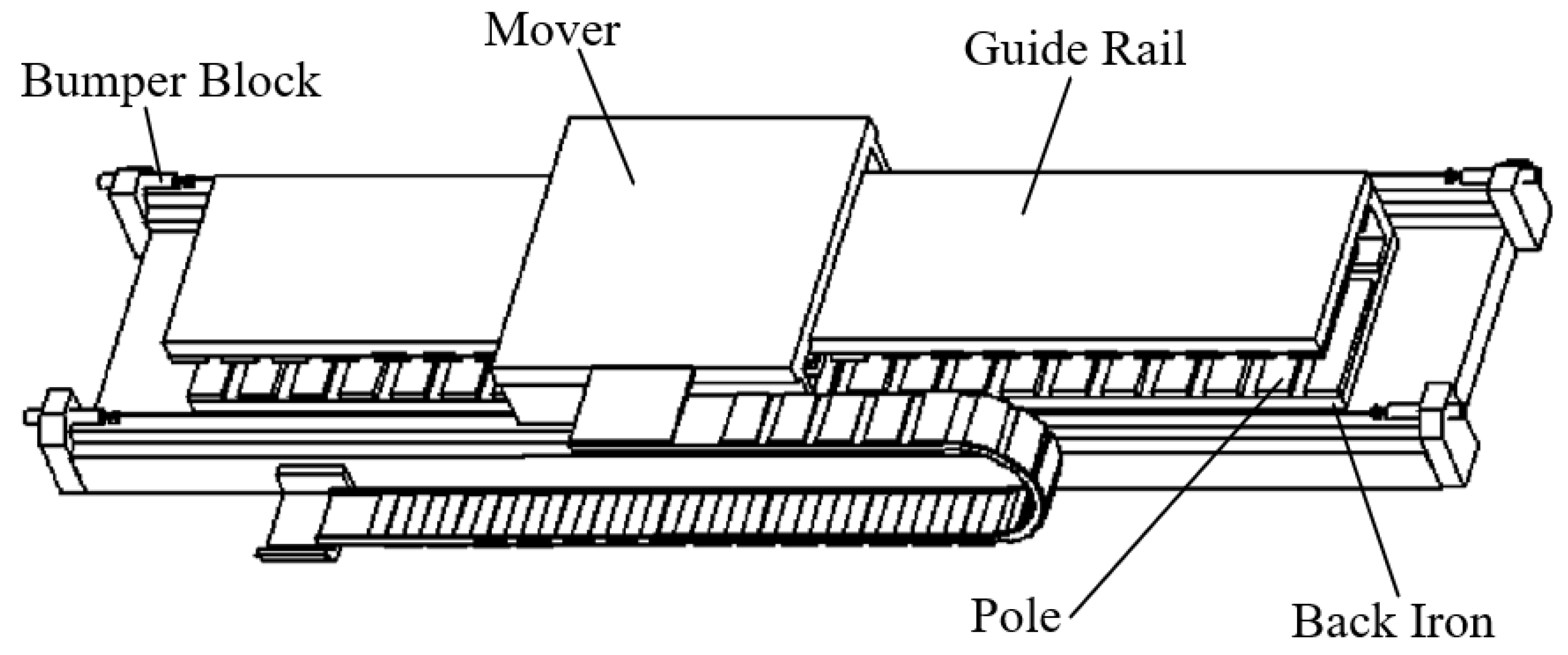
2. Mathematical Model of PMLSM

The basic structure of the PMLSM selected in this paper is shown in Figure 1.

A PMLSM is a strongly coupled, multivariable, nonlinear system. The voltage equation of a PMLSM can be obtained as:

$$\left\{\begin{array}{l}{u}_{\mathrm{d}}(t)=R_s{i}_{\mathrm{d}}+L_{\mathrm{d}}\frac{d{i}_{\mathrm{d}}}{dt}-\frac{\pi }{\tau }\nu {\psi }_{\mathrm{q}}\\ u_{\mathrm{q}}(t)=R_s{i}_{\mathrm{q}}+L_{\mathrm{q}}\frac{d{i}_{\mathrm{q}}}{dt}+\frac{\pi }{\tau }\nu {\psi }_{\mathrm{d}}\end{array}\right.$$

(1)

In the above formula, $R_s$ is the stator resistance of the PMLSM; $\tau$ is the pole distance of the PMLSM; $v$ is the running speed of the PMLSM; $u_{\mathrm{d}},u_{\mathrm{q}}$ are the voltage components of the $d-q$ axes of the PMLSM, respectively, $i_{\mathrm{d}},i_{\mathrm{q}}$ are the current components of $d-q$ axes of the PMLSM, respectively; $L_{\mathrm{d}},L_{\mathrm{q}}$ are the inductance components of $d-q$ axes of the PMLSM, respectively; and ${\psi }_{\mathrm{f}}$ is the permanent magnet flux of the PMLSM. The stator flux equation is:

$$\left\{\begin{array}{l}{\psi }_{\mathrm{d}}={\psi }_{\mathrm{f}}+L_{\mathrm{d}}{i}_{\mathrm{d}}\\ {\psi }_{\mathrm{q}}=L_{\mathrm{q}}{i}_{\mathrm{q}}\end{array}\right.$$

(2)

According to Formula (1), in the PMLSM, the current state equation is:

$$\left\{\begin{array}{l}\frac{d{i}_{\mathrm{d}}}{dt}=-\frac{R_{\mathrm{s}}}{L_{\mathrm{d}}}{i}_{\mathrm{d}}+\frac{\pi L_{\mathrm{q}}}{\tau L_{\mathrm{d}}}\nu i_{\mathrm{q}}+\frac{u_{\mathrm{d}}}{L_{\mathrm{d}}}\\ \frac{d{i}_{\mathrm{q}}}{dt}=-\frac{R_{\mathrm{s}}}{L_{\mathrm{q}}}{i}_{\mathrm{q}}-\frac{\pi L_{\mathrm{d}}}{\tau L_{\mathrm{q}}}\nu i_{\mathrm{d}}+\frac{u_{\mathrm{q}}}{L_{\mathrm{q}}}-\frac{\pi {\psi }_{\mathrm{f}}}{\tau L_{\mathrm{q}}}\nu \end{array}\right.$$

(3)

In the PMLSM, the equation of the electromagnetic thrust can be written as:

$$F_{\mathrm{em}}=\frac{3\mathsf{\pi }}{2\tau }{p}_{\mathrm{n}}[{\psi }_{\mathrm{f}}{i}_{\mathrm{q}}+(L_{\mathrm{d}}-L_{\mathrm{q}})i_{\mathrm{d}}{i}_{\mathrm{q}}]$$

(4)

In Formula (4), $F_{em}$ in the PMLSM is the thrust, and $p_n$ in the PMLSM is the number of pole pairs of the PMLSM. The PMLSM used in this paper, which satisfies $L_d=L_q=L$, the equation of the electromagnetic thrust can be written as:

$$F_{\mathrm{em}}=\frac{3\mathsf{\pi }}{2\tau }{i}_{\mathrm{q}}{p}_{\mathrm{n}}{\psi }_{\mathrm{f}}$$

(5)

The kinematical equation of PMLSM is:

$$m\frac{\mathrm{d}\nu }{\mathrm{d}t}=F_{\mathrm{em}}-F_f-B\nu$$

(6)

In Formula (6), $m$ is the mover’s mass in the PMLSM; $B$ in the PMLSM is the viscous friction factor; and $F_f$ is the system disturbance. Formulas (5) and (6) can be obtained simultaneously:

$$\frac{\mathrm{d}\nu }{\mathrm{d}t}=a_m{i}_{\mathrm{q}}+b_m\nu +c_m{F}_f$$

(7)

In the above formula, $a_{\mathrm{m}}=\frac{3\pi p_{\mathrm{n}}{\psi }_{\mathrm{f}}}{2m\tau }$, $b_{\mathrm{m}}=-\frac{B}{m}$, $c_{\mathrm{m}}=-\frac{1}{m}$.

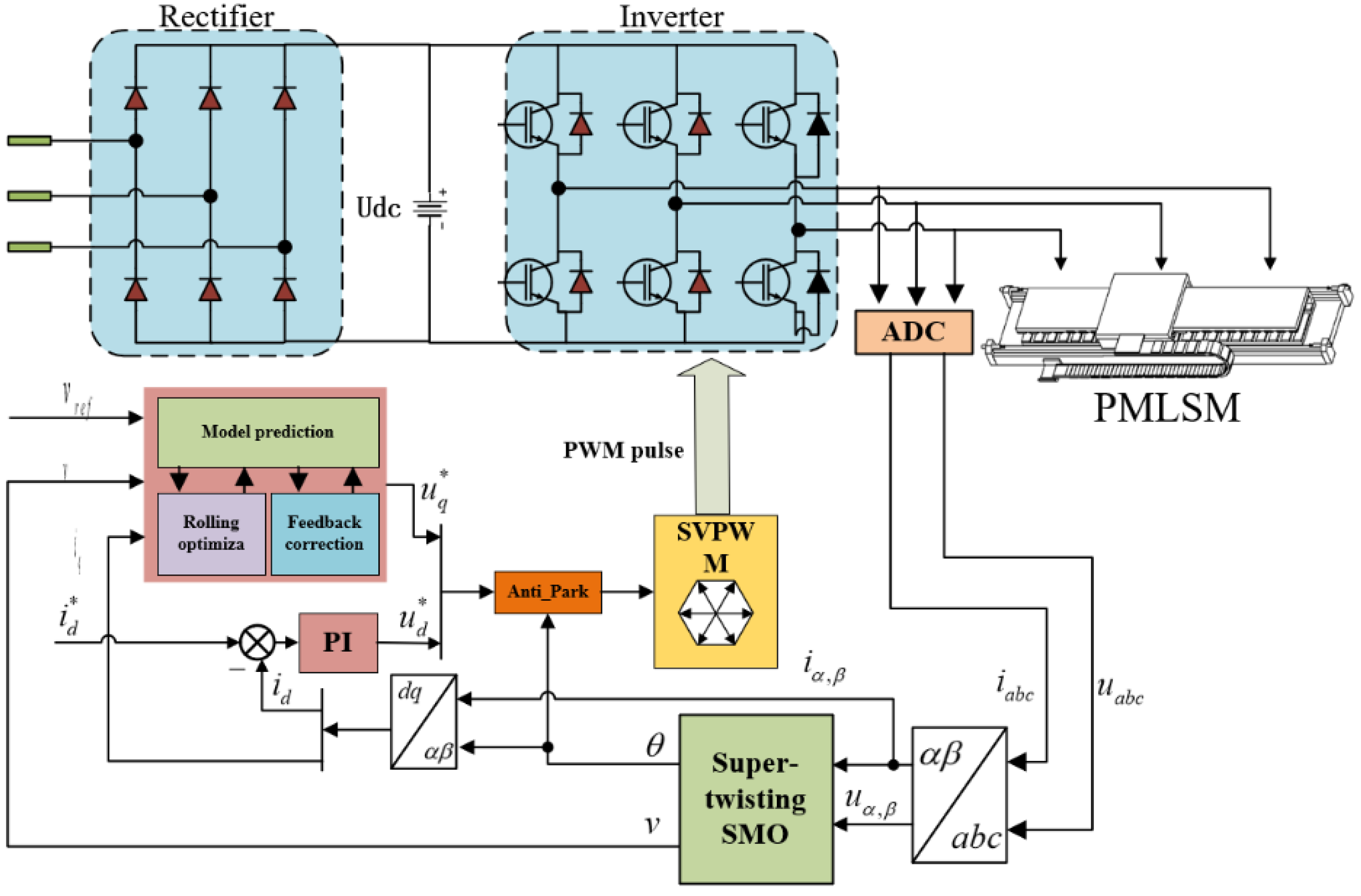
3. Speed and Current Integrated Controller

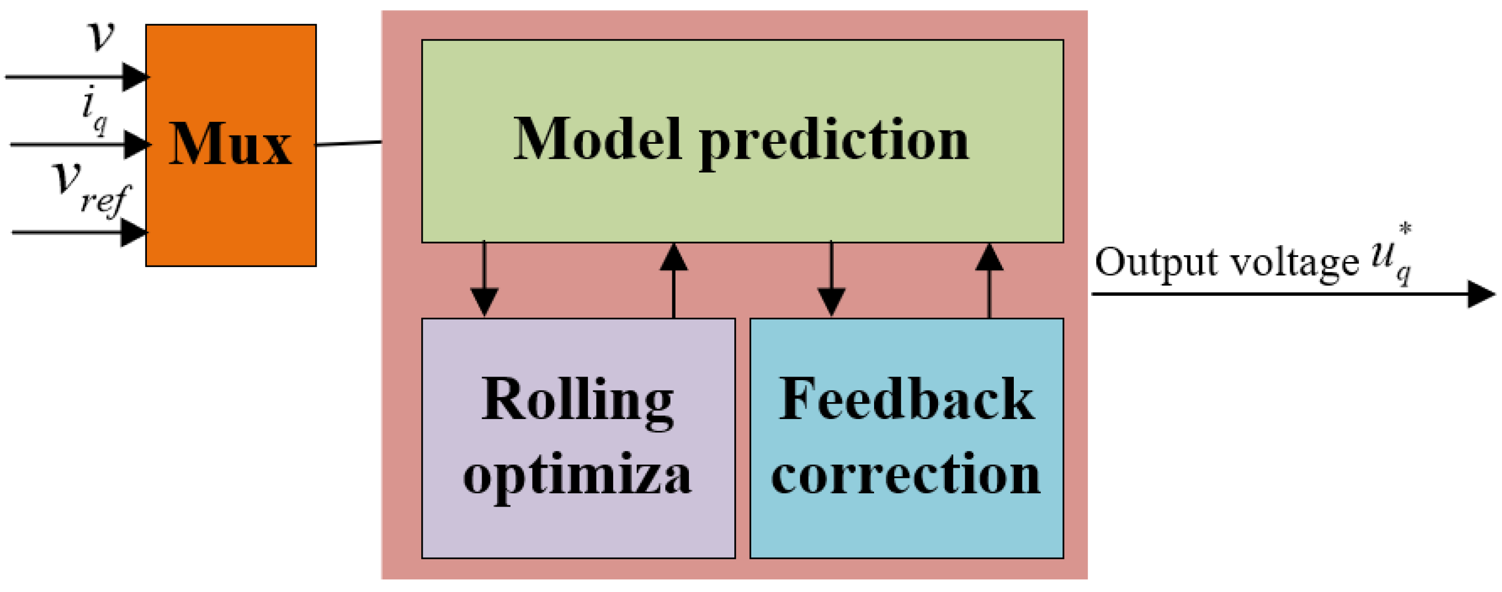
3.1. Design of the MPC Controller

According to the basic principle of model predictive control, the predictive model of PMLSM is derived from the mechanism of three steps: “predicting the future dynamics of the system → solving the optimization problem → the first element of the solution acts on the system” and “rolling time domain, repeating”. The optimization objective function is established, and the optimal control law is solved. From the implementation process of the MPC algorithm, for each output of the controlled object, the optimal control is generally calculated according to multiple predicted values, so it belongs to the category of multi-step or multi-value predictive control, in which the number of prediction steps and the length of the control time domain need to be selected, and the weighting coefficients of the output prediction error and control quantity in the index function in different periods need to be determined, which will increase the computational burden of the control system. It is difficult to apply to the fast time-varying motor-speed regulation system. The model predictive integrated controller designed in this paper improves the rolling optimization part on the basis of the traditional model predictive controller, and it takes a cycle number to calculate both the predictive time domain and the control time domain, so as to reduce the computational burden of the control system and better adapt to the fast-changing motor system. At the same time, the designed model predictive integrated controller simplifies the speed loop and current loop into a controller, which can directly output the expected value of the q-axis voltage. The design process of model predictive integrated controller is described in the following section.

3.1.1. Prediction Model

Without considering the load disturbance $F_f$, the Laplace transform is performed on both sides of Formula (6) to obtain the frequency domain model of the continuous system, as follows:

$$G(s)=\frac{V(s)}{I_q(s)}=\frac{K_m}{ms+B}$$

(8)

According to the Z-domain discretization method of the transfer function, the discrete Z-transfer function of the PMLSM is obtained by Formula (8) after zero-order sampling and holding:

$$G(z)=Z\left[\frac{1-e^{-Ts}}{s}\cdot \frac{K_m}{ms+B}\right]=\frac{\sigma z^{-1}}{1+\gamma z^{-1}}$$

(9)

In the above formula: ${\sigma }_0=K_m(1-e^{-TB/m})/B,\begin{array}{c}{\gamma }_0=-e^{-TB/m}\end{array}$; $T$ is the sampling time; and $K_{\mathrm{m}}=\frac{3\mathsf{\pi }}{2\tau }{p}_{\mathrm{n}}{\psi }_{\mathrm{f}}$.

According to Formula (9), the difference equation can be further obtained as:

$$\left\{\begin{array}{c}v(k)={\sigma }_0{i}_q(k-1)-{\gamma }_{0}v(k-1)\\ v(k+1)={\sigma }_0{i}_q(k)-{\gamma }_{0}v(k)\end{array}\right.$$

(10)

In the above formula, $v(k)$ is the actual speed of the PMLSM at $kT$ time.

The speed-prediction model of the PMLSM can be obtained by differentiating between the two equations in Formula (10):

$$v_m(k+1)=(1-{\gamma }_0)v(k)+{\gamma }_{0}v(k-1)+{\sigma }_0\Delta i_q^{*}(k)$$

(11)

In the above formula, $\Delta i_q^{*}(k)$ is the q-axis current control increment of the PMLSM at $kT$ time.

3.1.2. Closed-Loop Prediction and Reference Trajectory

Considering the influence of the unmodeled dynamic process, disturbance, and other uncertain factors on the output, the closed-loop predictive output of the system at time $(k+1)T$ can be obtained according to Formula (11):

$$v_p(k+1)=v_m(k+1)+e(k)$$

(12)

In Formula (12), the prediction error $e(k)=v(k)-v_m(k)$.

The reference trajectory is the expected output of the system that smoothly transitions from the current reality to the set value, generally in the form of a first-order exponential change, and the expression is as follows:

$$y(k+1)=\alpha v(k)+(1-\alpha )v_{ref}(k)$$

(13)

In the above formula, $\alpha$ is the softening coefficient—the smaller the value, the closer the reference trajectory is to the desired trajectory, but if the value is too small, the system will overshoot and oscillate. $v_{ref}(k)$ is the set value of the system.

3.1.3. Optimization Guidelines

In the control process, it is expected that the closed-loop predictive output $v_p(k+1)$ at the future time will be as close to the expected output $y(k+1)$, determined by the reference trajectory, as possible, and at the same time, it can ensure that the control increment $\Delta i_q^{*}(k)$ does not change too violently. Therefore, the secondary performance index is designed according to Formulas (12) and (13):

$$J_p=\lambda {[v_p(k+1)-y(k+1)]}^2+\beta {[\Delta i_q^{*}(k)]}^2$$

(14)

In the above formula, $\lambda ,\beta$ are weighting coefficients and respectively indicate the degree of the suppression of the tracking error and the control quantity change.

The optimal control law of the system is obtained by solving $\partial J_p/\partial \Delta i_q^{*}(k)=0$:

$$\Delta i_q^{*}(k)=-\frac{\lambda {\sigma }_0}{\lambda {\sigma }_0^2+\beta }[(1-{\gamma }_0)v(k)+{\gamma }_{0}v(k-1)+e(k)-y(k+1)]$$

(15)

Then, the given value of the q-axis current at $kT$ time is:

$$i_q^{*}(k)=i_q(k-1)+\Delta i_q^{*}(k)$$

(16)

Combining Formulas (3) and (7), ignoring the load disturbance $F_f$ and cross-coupling, and converting the q-axis current to the expected value, the equation for the reference voltage of the q-axis can be obtained as follows:

$$u_q^{*}(k)=[(\frac{a_m{L}_q}{R}\cdot \frac{d{i}_q^{*}(k)}{dt}+b_{m}v(k)-\frac{dv(k)}{dt})R_s]/a_m$$

(17)

The structural diagram of the above-modeled predictive integrated control is shown in Figure 2. The prediction model predicts the subsequent state variables according to the previous state variables and control variables. After the feedback correction, the predicted value and expected value of the motor speed are optimized through the secondary performance index to obtain the optimized control quantity, so as to realize the optimal control of the controlled object.

3.2. Stability Analysis of the MPC

Lyapunov stability theory is used to analyze the stability of the MPC controller of the PMLSM system. The stability is proven as follows: For a discrete system, the equation of state can be obtained as:

$$x(k+1)=G\cdot x(k)$$

(18)

The necessary and sufficient conditions for judging the asymptotic stability of the above equation of state are: For any given positive definite matrix $Q_1$, there is always a positive definite matrix $P$, which is the solution of the Lyapunov equation $G^T\cdot P\cdot G-P=-Q_1$ of the control system, and $V[x(k)]=x^T(k)\cdot P\cdot x(k)$ is the Lyapunov function of the control system.

For the integrated MPC controller designed in this paper, the space state equation of the MPC controller is:

$$\left\{\begin{array}{l}x(n+1)=A_m\cdot x(n)+B_m\cdot u(n)\\ y(n+1)=C_m\cdot x(n+1)\end{array}\right.$$

(19)

In the above formula, the state matrix is $x(n)={\left[\begin{array}{cc}i(n)& v(n)\end{array}\right]}^T$, the input is $u(n)=u_q(n)$, and the coefficient matrices are:

$$A_m=\left[\begin{array}{cc}1-\frac{R_s{T}_s}{L}& 0\\ a_m{T}_s& b_m{T}_s+1\end{array}\right], B_m=\left[\begin{array}{c}{T}_s/L\\ 0\end{array}\right], C_m=\left[\begin{array}{cc}1& 0\end{array}\right]$$

The coefficient matrix $A_m$ in the above formula is represented by $G$:

$$A_m=\left[\begin{array}{cc}1-\frac{R_s{T}_s}{L}& 0\\ a_m{T}_s& b_m{T}_s+1\end{array}\right]=G$$

(20)

Let positive definite matrix $Q=\left[\begin{array}{cc}1& 0\\ 0& 1\end{array}\right]$, matrix $P=P^T=\left[\begin{array}{cc}{P}_{11}& P_{12}\\ P_{12}& P_{22}\end{array}\right]$, sampling time $T_s=0.00001\mathrm{s}$, and substitute $Q,P$ into the Lyapunov equation $G^{\mathrm{T}}\cdot P\cdot G-P=-Q_1$ to obtain:

$$G^T\cdot \left[\begin{array}{cc}{P}_{11}& P_{12}\\ P_{12}& P_{22}\end{array}\right]\cdot G-\left[\begin{array}{cc}{P}_{11}& P_{12}\\ P_{12}& P_{22}\end{array}\right]=\left[\begin{array}{cc}-1& 0\\ 0& -1\end{array}\right]$$

(21)

The above formula can be obtained:

$$P=P^T=\left[\begin{array}{cc}108.5832& 32.0577\\ 32.0577& 166.6667\end{array}\right]$$

(22)

Due to $P_{11}=108.5832>0$ and $\det (P)=10769.5075>0$, the available matrix $P$ is a positive definite matrix. According to Lyapunov’s theorem, the MPC controller is asymptotically stable.

4. Super-Twisting Sliding-Mode Observer

4.1. Design of the Super-Twisting Sliding-Mode Observer

The realization principle of an ST-SMO is shown in Figure 3.

The super-twisting algorithm is:

$$\left\{\begin{array}{l}{d{x}_1/dt=-K_P\left|x_1-x_1^{*}\right|}^{1/2}\mathrm{sgn}\left(x_1-x_1^{*}\right)+x_2+{\rho }_1\\ d{x}_2/dt=-K_I\mathrm{sgn}\left(x_2-x_2^{*}\right)+{\rho }_2\end{array}\right.$$

(23)

Here, $x_1$ and $x_2$ are state variables, $x_1^{*}$ and $x_2^{*}$ are the estimated values of state variables, $\mathrm{sgn}$ is a symbolic function, $K_p$ and $K_I$ are the sliding-mode gain, and ${\rho }_1$ and ${\rho }_2$ are disturbance terms. According to [22], if ${\rho }_1$ and ${\rho }_2$ satisfy Formula (24), and $K_P$ and $K_I$ satisfy Formula (25), the control system will converge in a finite time:

$$\left\{\begin{array}{l}{\rho }_1\le a{\left|x_1\right|}^{1/2}\\ {\rho }_2=0\end{array}\right.$$

(24)

$a$ in the formula is any constant satisfying Formula (24):

$$\left\{\begin{array}{l}{K}_P>a{\left|x_1\right|}^{1/2}\\ K_I>(5a{K}_P^2+4K_P{a}^2)/2(K_P-2a)\end{array}\right.$$

(25)

The design of the SMO algorithm is based on the mathematical model of $\alpha -\beta$ axis in the PMLSM, so we rewrite the voltage equation of the PMLSM as follows:

$$\left[\begin{array}{l}{u}_{\mathsf{\alpha }}\\ u_{\mathsf{\beta }}\end{array}\right]=\left[\begin{array}{cc}{R}_s+p{L}_{\mathrm{d}}& {\omega }_{\mathrm{e}}{L}_{\mathrm{d}}-{\omega }_{\mathrm{e}}{L}_{\mathrm{q}}\\ -{\omega }_{\mathrm{e}}{L}_{\mathrm{d}}+{\omega }_{\mathrm{e}}{L}_{\mathrm{q}}& R_s+p{L}_{\mathrm{d}}\end{array}\right]\left[\begin{array}{l}{i}_{\mathsf{\alpha }}\\ i_{\mathsf{\beta }}\end{array}\right]+\left[\begin{array}{l}{E}_{\mathsf{\alpha }}\\ E_{\mathsf{\beta }}\end{array}\right]$$

(26)

In Formula (26), $u_{\alpha }$, $u_{\beta }$ are the stator voltages; $i_{\alpha }$, $i_{\beta }$ are the stator currents; $E_{\alpha }$, $E_{\beta }$ are the extended back EMF; ${\omega }_e$ represents electrical angular velocity; and $p$ is a differential operator and satisfies:

$$\left[\begin{array}{l}{E}_{\mathsf{\alpha }}\\ E_{\mathsf{\beta }}\end{array}\right]=\left[(L_{\mathrm{d}}-L_{\mathrm{q}})({\omega }_{\mathrm{e}}{i}_{\mathrm{d}}-p{i}_{\mathrm{q}})+{\omega }_{\mathrm{e}}{\psi }_{\mathrm{f}}\right]\left[\begin{array}{l}-\sin {\theta }_{\mathrm{e}}\\ \cos {\theta }_{\mathrm{e}}\end{array}\right]$$

(27)

For the PMLSM used, $L_d=L_q=L$, so Formula (27) of the extended back EMF can be simplified to a variable only related to the motor speed. The higher the speed, the greater the back EMF. For the convenience of observation, Formulas (26) and (27) can be changed to:

$$\left\{\begin{array}{l}\frac{d{i}_{\mathsf{\alpha }}}{dt}=-\frac{R_s{i}_{\mathsf{\alpha }}-u_{\mathsf{\alpha }}+E_{\mathsf{\alpha }}}{L}\\ \frac{d{i}_{\mathsf{\beta }}}{dt}=-\frac{R_s{i}_{\mathsf{\beta }}-u_{\mathsf{\beta }}+E_{\mathsf{\beta }}}{L}\end{array}\right.$$

(28)

$$\left\{\begin{array}{l}{E}_{\mathsf{\alpha }}=-{\psi }_{\mathrm{f}}{\omega }_{\mathrm{e}}\sin {\theta }_{\mathrm{e}}\\ E_{\mathsf{\beta }}={\psi }_{\mathrm{f}}{\omega }_{\mathrm{e}}\cos {\theta }_{\mathrm{e}}\end{array}\right.$$

(29)

In the above formula, ${\theta }_e=P_n\theta$ and $P_n$ are the number of poles of the motor. To realize the sensorless control strategy, $\omega$ and ${\theta }_e$ need to be estimated, and the symbol “^” represents the observed value. Then, it is given that the dynamic estimation error is $\widetilde{i_{\alpha }}={\widehat{i}}_{\alpha }-i_{\alpha }$, $\widetilde{i_{\beta }}={\widehat{i}}_{\beta }-i_{\beta }$. Substituting ${\widehat{i}}_{\alpha }$ and ${\widehat{i}}_{\beta }$ as system variables into Formula (23), a current observer based on the ST-SMO is established as follows:

$$\frac{d}{dt}\left[\begin{array}{l}{\widehat{i}}_{\alpha }\\ {\widehat{i}}_{\beta }\end{array}\right]=\left[\begin{array}{l}-K_{\mathrm{P}}{\left|\widetilde{i_{\mathsf{\alpha }}}\right|}^{1/2}\mathrm{sgn}(\widetilde{i_{\mathsf{\alpha }}})-{\displaystyle \int K_{\mathrm{I}}\mathrm{sgn}(\widetilde{i_{\mathsf{\alpha }}})dt+{\rho }_{\mathsf{\alpha }}}\\ -K_{\mathrm{P}}{\left|\widetilde{i_{\mathsf{\beta }}}\right|}^{1/2}\mathrm{sgn}(\widetilde{i_{\mathsf{\beta }}})-{\displaystyle \int K_{\mathrm{I}}\mathrm{sgn}(\widetilde{i_{\mathsf{\beta }}})dt+{\rho }_{\mathsf{\beta }}}\end{array}\right]$$

(30)

The disturbance term in the formula is:

$$\left[\begin{array}{l}{\rho }_{\mathsf{\alpha }}\\ {\rho }_{\mathsf{\beta }}\end{array}\right]=\left[\begin{array}{c}(u_{\mathsf{\alpha }}-R_s{\widehat{i}}_{\alpha })/L\\ (u_{\mathsf{\beta }}-R_s{\widehat{i}}_{\beta })/L\end{array}\right]$$

(31)

4.2. Proof of Stability

By substituting Formula (31) into Formula (24), we obtain:

$$\left\{\begin{array}{l}(u_{\mathsf{\alpha }}-R_s{\widehat{i}}_{\alpha })/L-a{\left|{\widehat{i}}_{\alpha }\right|}^{1/2}\le 0\\ (u_{\mathsf{\beta }}-R_s{\widehat{i}}_{\beta })/L-a{\left|{\widehat{i}}_{\beta }\right|}^{1/2}\le 0\end{array}\right.$$

(32)

Obviously, when $a$ is large enough, the stability condition is satisfied. The difference between Formula (30) and Formula (28) can be obtained:

$$\frac{d}{dt}\left[\begin{array}{l}\widetilde{i_{\mathsf{\alpha }}}\\ \widetilde{i_{\mathsf{\beta }}}\end{array}\right]=-\frac{R_s}{L}\left[\begin{array}{l}\widetilde{i_{\mathsf{\alpha }}}\\ \widetilde{i_{\mathsf{\beta }}}\end{array}\right]+\frac{1}{L}\left[\begin{array}{l}{E}_{\mathsf{\alpha }}\\ E_{\mathsf{\beta }}\end{array}\right]-\left[\begin{array}{l}{K}_P{\left|\widetilde{i_{\mathsf{\alpha }}}\right|}^{1/2}\mathrm{sgn}(\widetilde{i_{\mathsf{\alpha }}})+{\displaystyle \int K_I\mathrm{sgn}(\widetilde{i_{\mathsf{\alpha }}})dt}\\ K_P{\left|\widetilde{i_{\mathsf{\beta }}}\right|}^{1/2}\mathrm{sgn}(\widetilde{i_{\mathsf{\beta }}})+{\displaystyle \int K_I\mathrm{sgn}(\widetilde{i_{\mathsf{\beta }}})dt}\end{array}\right]$$

(33)

The inverse electromotive force can be obtained from the equivalence principle:

$$\left[\begin{array}{l}{E}_{\mathsf{\alpha }}\\ E_{\mathsf{\beta }}\end{array}\right]=L\left[\begin{array}{l}{K}_P{\left|\widetilde{i_{\alpha }}\right|}^{1/2}\mathrm{sgn}(\widetilde{i_{\alpha }})+{\displaystyle \int K_I\mathrm{sgn}(\widetilde{i_{\alpha }})dt}\\ K_P{\left|\widetilde{i_{\beta }}\right|}^{1/2}\mathrm{sgn}(\widetilde{i_{\beta }})+{\displaystyle \int K_I\mathrm{sgn}(\widetilde{i_{\beta }})dt}\end{array}\right]$$

(34)

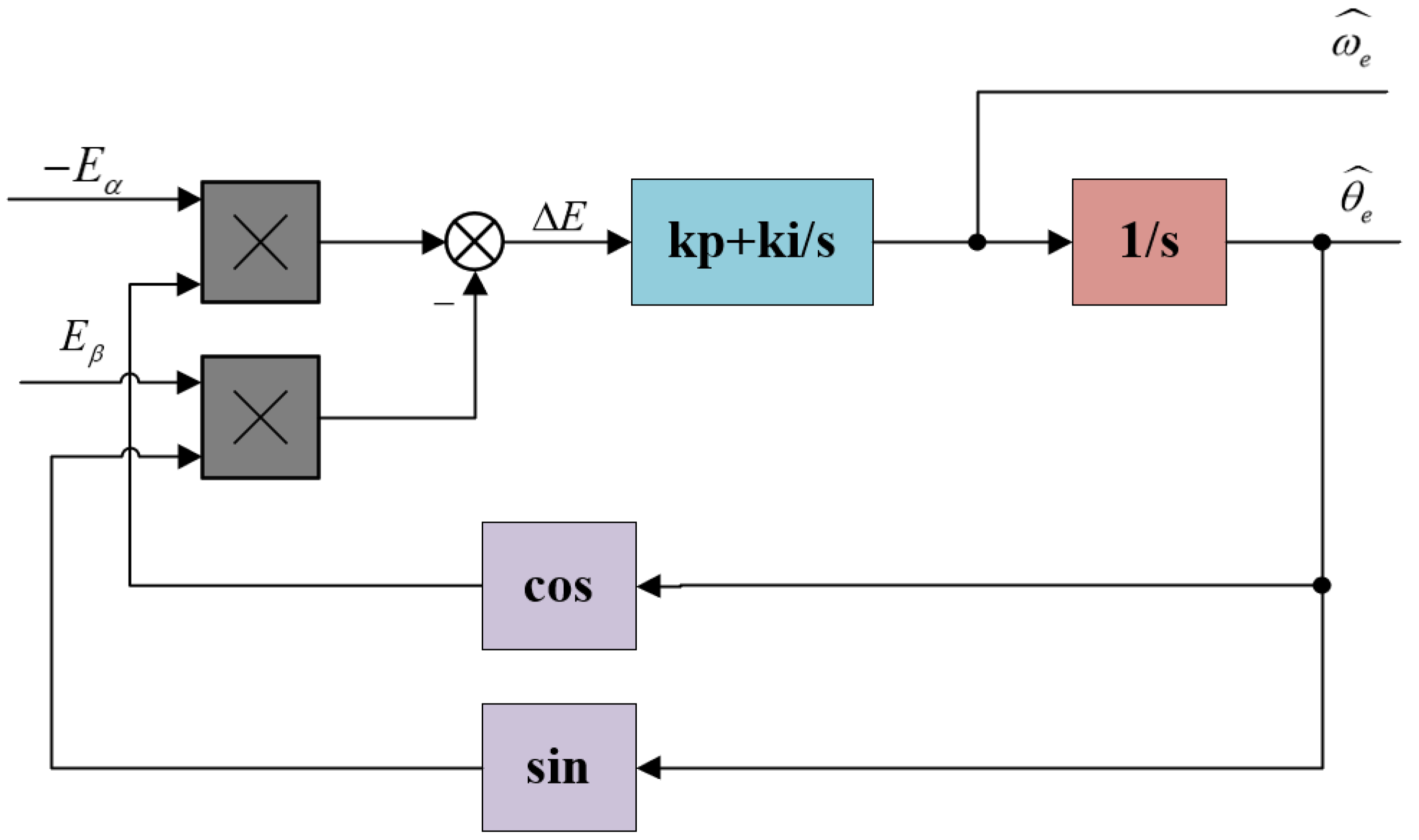
4.3. PLL Strategy Application

The traditional estimation method based on the arctangent function will directly substitute chattering in sliding-mode into the calculation, which will lead to an increase in estimation error. In this paper, the PLL system is used to extract position information, as shown in Figure 4.

Hypothesis:

$$k=(L_{\mathrm{d}}-L_{\mathrm{q}})({\omega }_{\mathrm{e}}{i}_{\mathrm{d}}-p{i}_{\mathrm{q}})+{\widehat{\omega }}_e{\psi }_{\mathrm{f}}$$

(35)

Due to $L_d=L_q=L$ in the motor used, the above formula can be simplified as:

$$k={\widehat{\omega }}_e{\psi }_{\mathrm{f}}$$

(36)

In a traditional PLL, the position error signal is:

$$\begin{array}{ll}\Delta E& =-E_{\mathsf{\alpha }}\cos {\widehat{\theta }}_e-E_{\mathsf{\beta }}\sin {\widehat{\theta }}_e\\ & =k\sin {\theta }_{\mathrm{e}}\cos {\widehat{\theta }}_e-k\cos {\theta }_{\mathrm{e}}\sin {\widehat{\theta }}_e\\ & =k\sin ({\theta }_{\mathrm{e}}-{\widehat{\theta }}_e)\end{array}$$

(37)

When the system approaches the steady-state, the value of $\left|{\theta }_e-{\widehat{\theta }}_e\right|$ is minimal. Assuming $\sin \left({\theta }_e-{\widehat{\theta }}_e\right)={\theta }_e-{\widehat{\theta }}_e$, after normalization, the position signal error is:

$$\Delta \overline{E}=\frac{\Delta E}{\sqrt{E_{\mathsf{\alpha }}^2+E_{\mathsf{\beta }}^2}}=\frac{k\left({\theta }_{\mathrm{e}}-{\widehat{\theta }}_e\right)}{\sqrt{E_{\mathsf{\alpha }}^2+E_{\mathsf{\beta }}^2}}={\theta }_{\mathrm{e}}-{\widehat{\theta }}_e$$

(38)

Therefore, the PLL closed-loop transfer function from ${\widehat{\theta }}_e$ to ${\theta }_{\mathrm{e}}$ is:

$$G\left(s\right)=\frac{{\widehat{\theta }}_e}{{\theta }_{\mathrm{e}}}=\frac{2\xi {\omega }_{\mathrm{n}}s+{\omega }_{\mathrm{n}}^2}{s^2+2\xi {\omega }_{\mathrm{n}}s+{\omega }_{\mathrm{n}}^2}$$

(39)

where $\xi =\sqrt{k{k}_i}$, ${\omega }_n=(k_p/2)\sqrt{k/k_i}$, where ${\omega }_n$ determines the bandwidth of the PI regulator, and $k_p$ and $k_i$ are normal numbers.

5. Traditional SMC Controller

5.1. Design of a Traditional SMC Controller

In order to better reflect the control performance of the designed model predictive integrated controller, a traditional SMC controller is selected for comparison. The specific design is as follows:

$$\left\{\begin{array}{c}{z}_{m1}=v_{ref}-v\\ z_{m2}={\dot{z}}_{m1}=-\dot{v}\end{array}\right.$$

(40)

Since $Bv$ in Formula (6) is too small, it can be ignored. Substitute Formula (3) and Formula (6) into the above formula to obtain:

$$\left\{\begin{array}{c}{\dot{z}}_{m1}=-\dot{v}=\frac{1}{m}(F_f-\frac{3\pi p_n{\psi }_f}{2\tau }{i}_q)\\ {\dot{z}}_{m2}={\ddot{z}}_{m1}=-\ddot{v}=-\frac{3\pi p_n{\psi }_f}{2\tau m}{i}_q\end{array}\right.$$

(41)

Define $u_m={\dot{i}}_q,\begin{array}{c}{D}_m=\frac{3\pi p_n{\psi }_f}{2\tau m}\end{array}$. Then, there are:

$$\left[\begin{array}{c}{\dot{z}}_{m1}\\ {\dot{z}}_{m2}\end{array}\right]=\left[\begin{array}{cc}0& 1\\ 0& 0\end{array}\right]\left[\begin{array}{c}{z}_{m1}\\ z_{m2}\end{array}\right]+\left[\begin{array}{c}0\\ -D_m\end{array}\right]u_m$$

(42)

The sliding surface is designed as follows:

$$s_m=l_m{z}_{m1}+z_{m2}$$

(43)

In the above formula, $l_m$ is the control parameter greater than zero. Derivation of the above formula can be obtained:

$${\dot{s}}_m=l_m{\dot{z}}_{m1}+{\dot{z}}_{m2}=l_m{z}_{m2}+{\dot{z}}_{m2}=l_m{z}_{m2}-D_m{u}_m$$

(44)

In order to ensure that the PMLSM system has good dynamic performance, the exponential approach method is used here, and the available expression is:

$$u_m={\dot{i}}_q=\frac{1}{D_m}\left[l_m{z}_{m2}+\epsilon \mathrm{sgn}(s_m)+q_m{s}_m\right]$$

(45)

Further, the reference current of the q-axis can be obtained as:

$$i_q^{*}=\frac{1}{D_m}{\displaystyle {\int }_0^t\left[l_m{z}_{m2}+\epsilon \mathrm{sgn}(s_m)+q_m{s}_m\right]dt}$$

(46)

It can be seen from the above formula that, since the controller includes an integral term, on the one hand, the chattering phenomenon can be reduced, and on the other hand, the steady-state error of the system can be eliminated, and the controller can improve the quality of the system.

5.2. Stability Analysis of a Traditional SMC Controller

Choose the Lyapunov function as:

$$V_m=\frac{1}{2}{s}_m^2$$

(47)

The derivation of the above formula can be obtained:

$$\begin{array}{ll}{\dot{V}}_m& =s_m{\dot{s}}_m\\ & =s_m[-\epsilon \mathrm{sgn}(s_m)-q_m{s}_m]\\ & =-\epsilon s_m\mathrm{sgn}(s_m)-q_m{s}_m^2\\ & =-\epsilon \left|s_m\right|-q_m{s}_m^2\\ & <0\end{array}$$

(48)

According to Lyapunov stability theory, a traditional SMC controller design is asymptotically stable.

6. Simulation and Experimental Results

6.1. System Simulation

The block diagram of the sensorless PMLSM vector system design based on the integrated controller of the integrated predictive speed and current is shown in Figure 5. The system simulation model designed in this paper was established according to the PMLSM driving parameters in

Table 1. Main parameters of the motor.

Parameter	Value
stator resistance Rs/Ω	4.0
d–q axis inductance Ldq/mH	8.2
Mover mass m/kg	1.425
Viscous friction coefficient B/N/m·s	44
Polar distance τ/m	0.016

, and the operation conditions of the PMLSM’s speed and current are compared under the conditions of speed regulation and variable load. The control performance of the model prediction integrated controller, the sliding-mode controller (SMC), and the PI controller are analyzed. Then, an observer is added to the proposed model predictive integrated controller, and the speed-tracking performance of the proposed ST-SMO is compared with that of the SMO. The system sampling time during simulation is 1 μs.

In this paper, the parameters of the controller are selected by the empirical tuning method and the Ziegler–Nichols method. In order to ensure the better control effect of the controller, the overshoot and adjustment time are used as the basis to select the parameters for many times, and the data with better effect is selected as the final parameter. We keep the current loop parameters of the PI system and the SMC system the same. The parameters used in the PI controller in the speed loop are: $K_{P1}=1.8,K_{I1}=20$. The parameters used in the SMC controller are: $l_m=15,\epsilon =600,q_m=800$. The parameters used in the MPC controller are: $\alpha =0.999,\lambda =5000,\beta =0.0175$. The parameters used in the ST-SMO in this paper are: $K_P=450,K_I=300,k_p=20,k_i=450$.

The PI-controller parameter tuning process is as follows: In the parameter tuning of PI controller, the Ziegler–Nichols tuning method is used to quickly and efficiently determine the optimal parameter value of the PI controller. The stability limit is determined by adjusting the proportional coefficient $K_{P1}$, and the critical coefficient and critical oscillation period are obtained. $K_{P1}$ and $K_{I1}$, at this time, can be calculated according to the calculation formula of the PI controller in the Ziegler–Nichols tuning method. Due to interference factors, such as cross-coupling terms in the actual permanent magnet linear synchronous motor system, the parameters calculated by the Ziegler–Nichols setting method still need to be adjusted according to the actual situation, so as to finally obtain the above PI-controller parameter values.

The SMC-controller parameter tuning process is as follows: The second-order sliding-mode surface used in this paper is: $s_m=l_m{z}_{m1}+{\dot{z}}_{m1}$. Since this equation has both $z_{m1}$ and ${\dot{z}}_{m1}$, it approximates an inertial system: $G(s)=1/(Ts+1)$. The time domain equation corresponding to the transfer function $G(s)$ is: $y(t)=T\dot{x}(t)+x(t)$. According to classic automatic control theory, when the system contains an inertial system, the system will have a steady-state response component: $x_i(t)=k{e}^{-t/T}$. This function is a monotonically decreasing, exponential function, which ensures the stability and boundedness of the system. Taking the second-order sliding-mode surface as an inertial system, the parameter adjustment method of the SMC controller is obtained: The adjustment parameter, $l_m$, is the main parameter, and the larger its value is, the faster the system will reach steady state. However, too large a value will also cause the system to oscillate. After determining $l_m$, the other two parameters can be adjusted. In the exponential approach rate, ${\dot{s}}_m=-\epsilon \mathrm{sgn}(s_m)-q_m{s}_m$, increasing $\epsilon$ and $q_m$ can speed up the system response time and reduce the overshoot, but too large of an increase will make the system chatter and increase the error. Finally, according to the above-described derivation process, nearly optimal SMC controller parameters can be obtained.

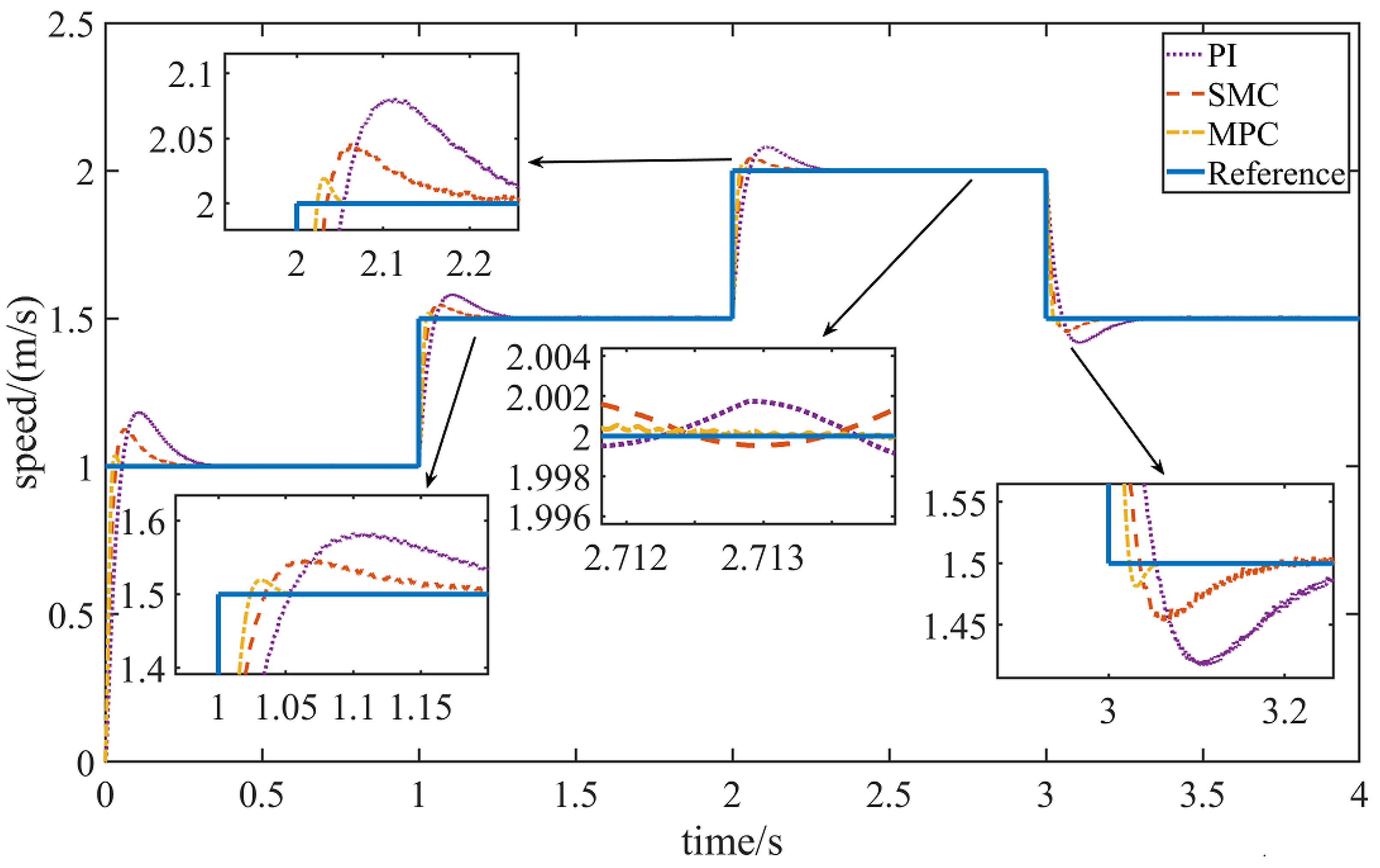
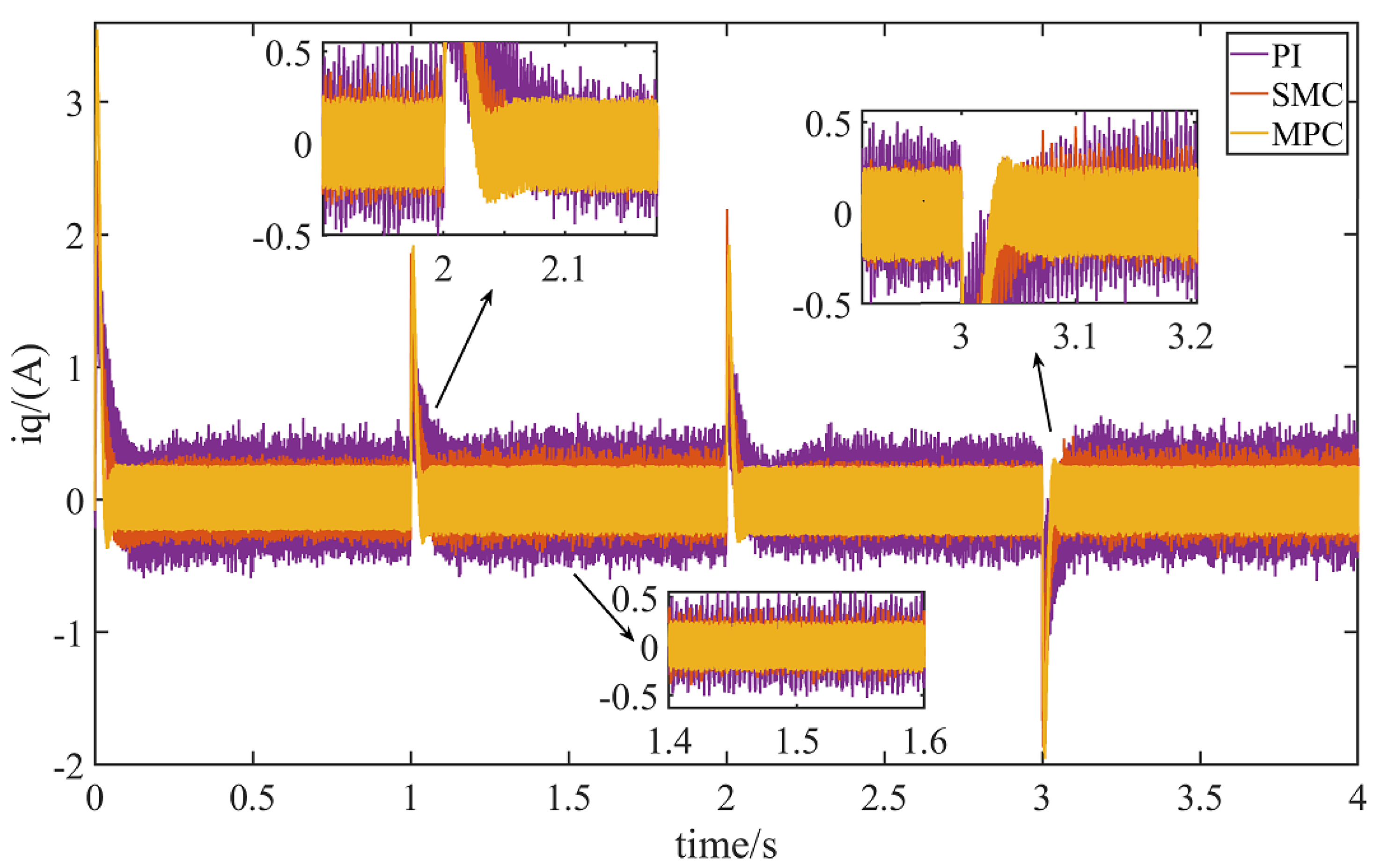
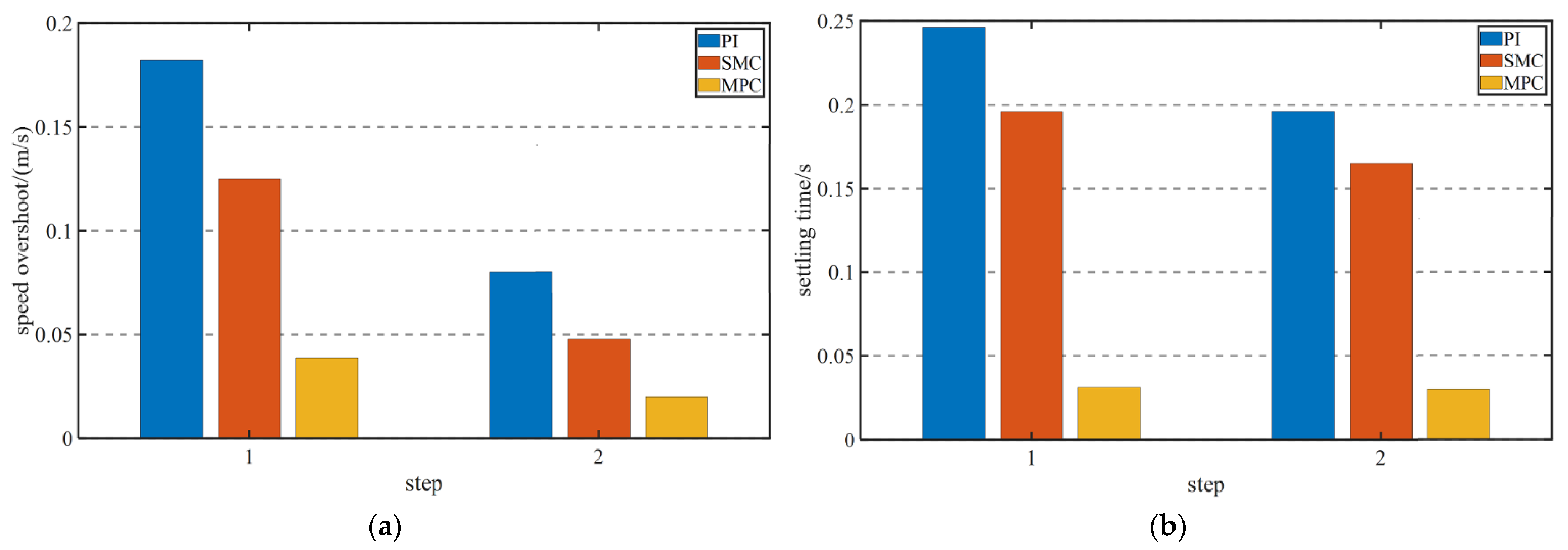
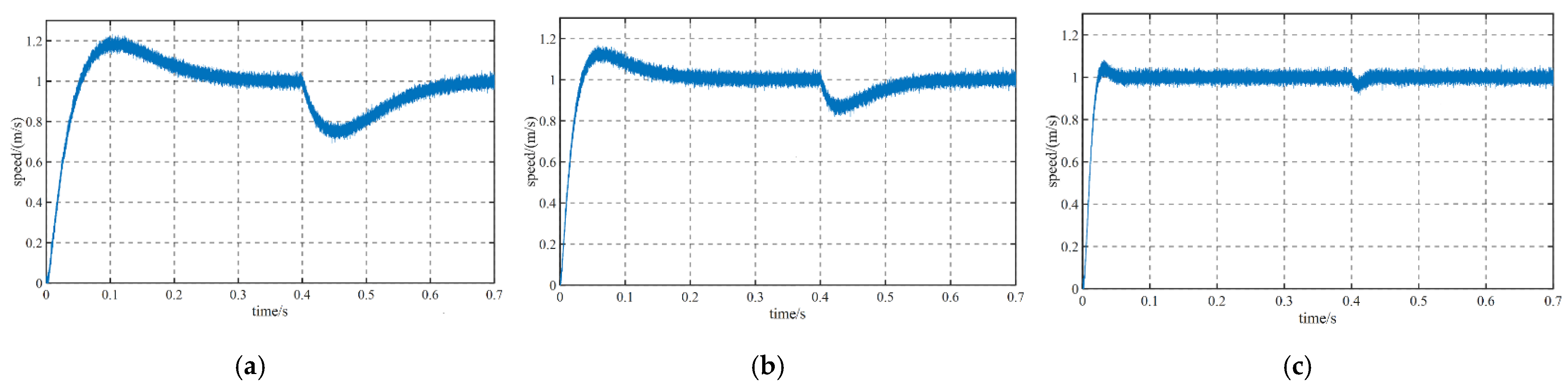
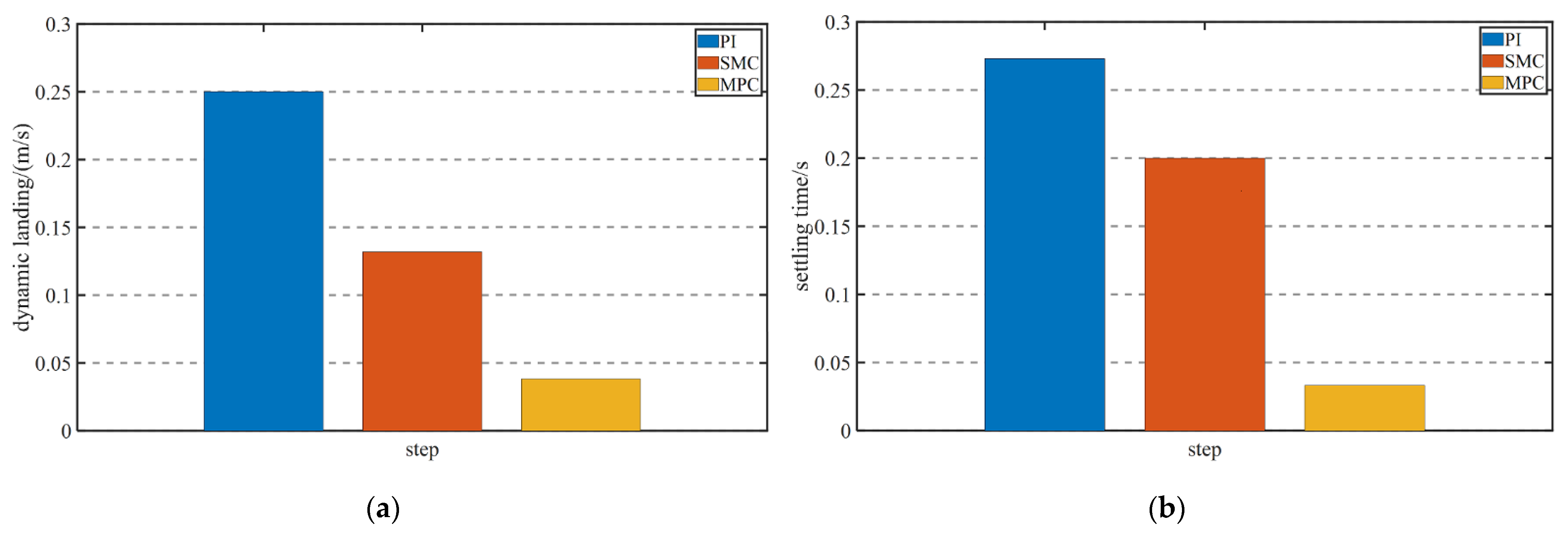
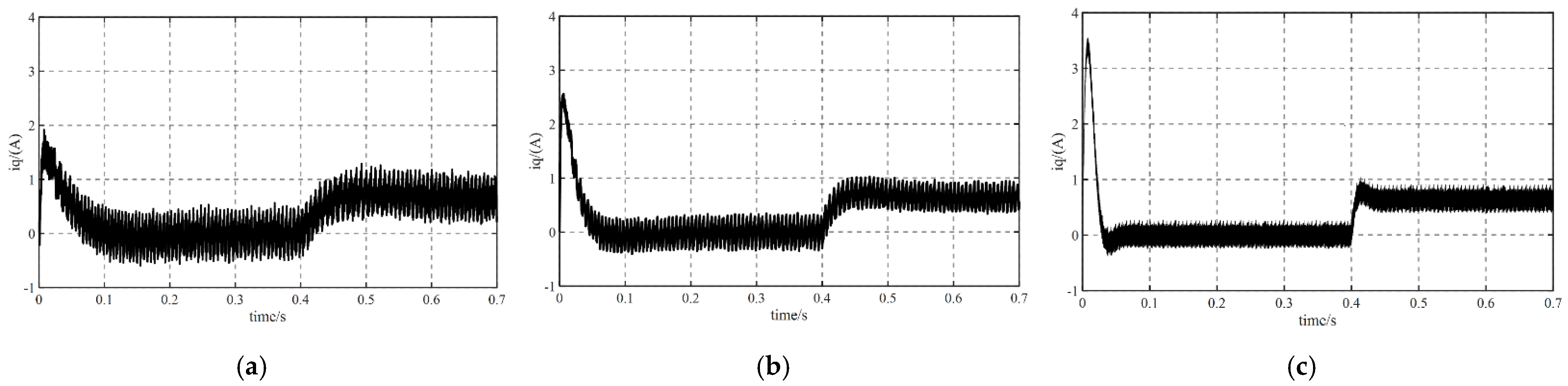
6.1.1. The Load Remains Unchanged, and the Speed Changes

The given speed of the PMLSM control system changes every 1 s, and the change condition is $1 \mathrm{m}/\mathrm{s}\to 1.5 \mathrm{m}/\mathrm{s}\to 2 \mathrm{m}/\mathrm{s}\to 1.5 \mathrm{m}/\mathrm{s}$. Figure 6 shows the running-speed waveform of the PMLSM at the MPC controller, the PI controller, and the SMC controller. In Figure 6, we can observe the running-speed waveforms of the control system as they rise and fall.

According to Figure 6, the MPC system in this design not only has a smaller overshoot, but it also greatly shortens the regulation time compared with the SMC system and the PI system under the condition of motor speed increase or decrease. In the high-speed operation stage of 2 m/s, the MPC system has less jitter and stronger stability.

Figure 7 shows the q-axis current waveforms of the PMLSM of the three systems under variable speed. In the process of a sudden speed change, the MPC system can mobilize a larger current to ensure a fast tracking-speed in a short time, and the adjustment time is about 0.03 s. During the sudden change of speed, the PI system cannot quickly adjust the current to make the system achieve the desired effect. The adjustment time is about 0.12 s, which is 4 times that of the MPC system. And the adjustment time of the SMC system is about 0.07 s, which is about twice that of the MPC system.

When the speed is stable, the current waveform of the MPC system has less jitter and is more stable than either the PI system or the SMC system, and the jitter amplitude of the current waveform is about 0.4 A. When the speed is stable, the current waveform of the PI system has more jitter, and the jitter amplitude is about 0.8 A, which is twice that of the MPC system. Additionally, the jitter amplitude of the SMC system is about 0.6 A, which is about 1.5 times that of the MPC system.

The simulation analysis of variable-speed motion proves that the model predictive integrated control system proposed in this paper has superior dynamic control performance.

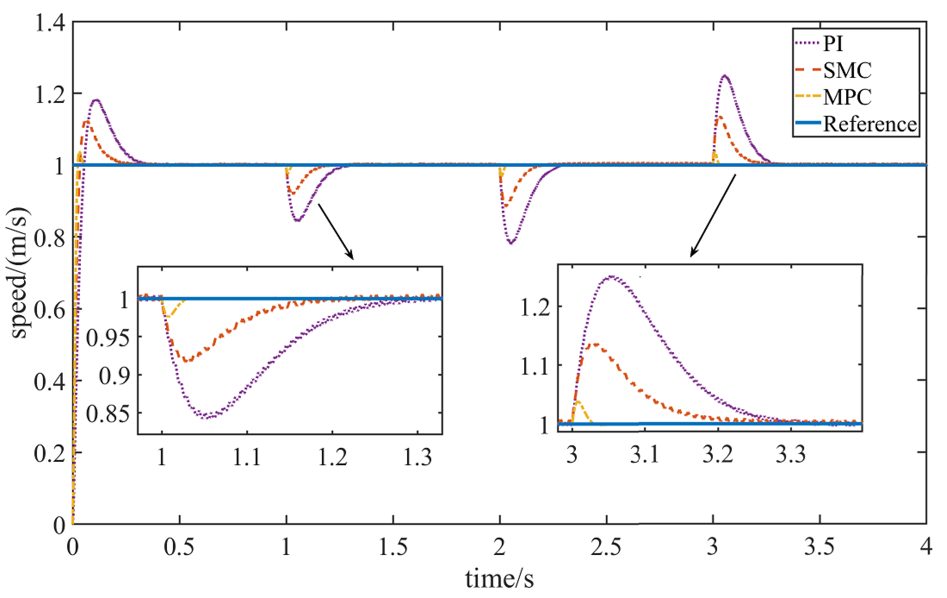
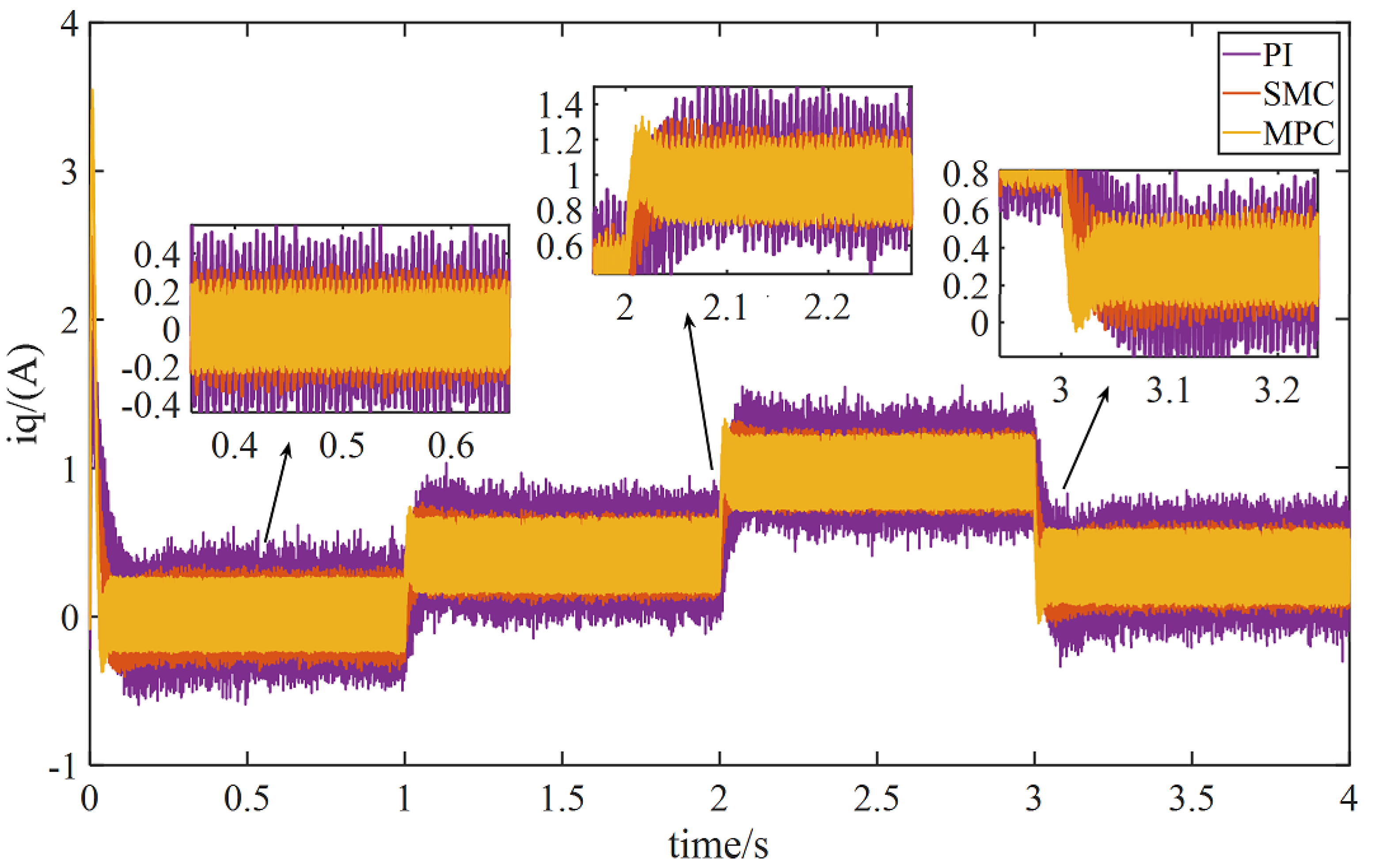
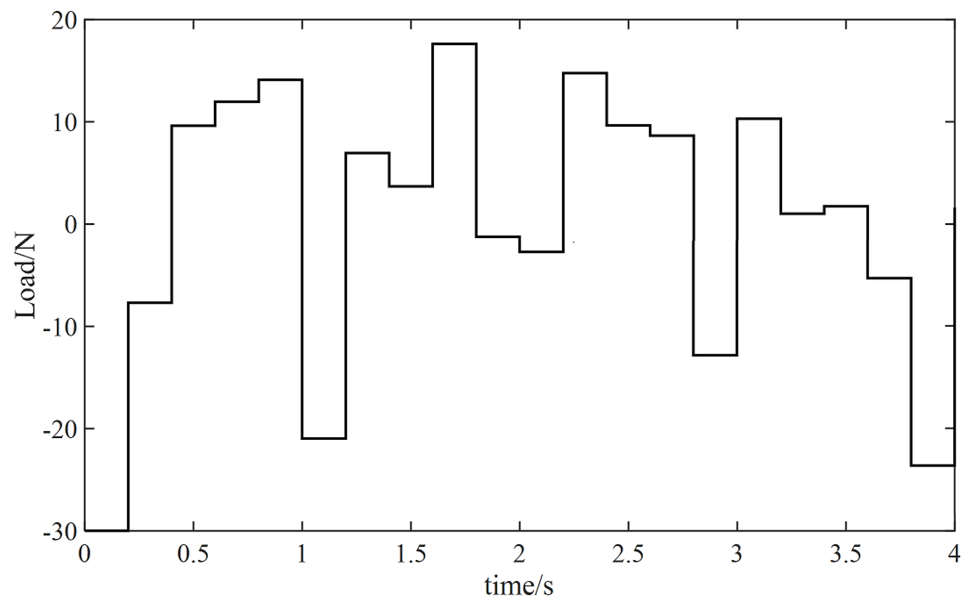
6.1.2. The Speed Remains Unchanged and the Load Changes

The given speed of the linear motor system is 1 m/s. The load is changed during the operation of the system, and the change of the added load value is $50\mathrm{N}\to 70\mathrm{N}\to 80\mathrm{N}$. This is used to compare the changes of the speed and current in the MPC system, the PI system, and the SMC system under the condition of a sudden load increase and a sudden drop so as to analyze their anti-disturbance performance.

In Figure 8, when the added load is 50 N, the speed change of the MPC system is about 0.04 m/s, and the adjustment time is about 0.05 s. The speed variation of the PI system is about 0.16 m/s, which is 4 times that of the MPC system. The adjustment time of the PI system is about 0.3 s, which is 6 times that of the MPC system. The speed variation of the SMC system is about 0.08 m/s, which is 2 times that of the MPC system. The adjustment time of the SMC system is about 0.2 s, which is 4 times that of the MPC system.

When the added load is 80 N, the speed change of the MPC system is about 0.05 N, and the adjustment time is about 0.06 s. The speed variation of the PI system is about 0.28 N, which is about 6 times that of the MPC system. The adjustment time of the PI system is about 0.3 s, which is 5 times that of the MPC system. The speed variation of the SMC system is about 0.13 m/s, which is 3 times that of the MPC system. The adjustment time of the SMC system is about 0.25 s, which is 4 times that of the MPC system.

According to Figure 8, in the case of a sudden increase or decrease in load, the velocity fluctuation and adjustment time of the MPC system are far less than that of the PI system and the SMC system.

A variable load is added to the PI system, the SMC system, and the designed MPC system, and the current waveform changes and comparisons in the 3 control systems are shown in Figure 9. During a sudden change of load, the PI system and the SMC system cannot adjust the current quickly enough to make the system achieve the desired effect. The adjustment time of the PI system is about 0.14 s, which is about 3 times that of the MPC system. The adjustment time of the SMC system is about 0.09 s, which is about twice that of the MPC system. Compared with the PI system and the SMC system, the MPC system can mobilize a larger current in a shorter time to ensure a fast tracking-speed, and the adjustment time is about 0.04 s.

When the speed remains stable, the current waveform jitter of the PI system is greater, and the jitter amplitude is about 0.8 A, which is twice that of the MPC system. The jitter amplitude of the SMC system is about 0.6 A, which is about 1.5 times that of the MPC system. Compared with the PI system and the SMC system, the current waveform of the MPC system has less and more-stable jitter, and the jitter amplitude of the current waveform is about 0.4 A.

In order to better verify the anti-disturbance ability and control performance of the designed MPC system in a complex environment, the random load in Figure 10 is added to the 3 systems.

Figure 11 shows the comparison of the operation-speed waveforms of the 3 control systems with random loads when the operation speeds were set at 1 m/s. As the random load changes once every 0.2 s, the speed waveforms of PI system and SMC system change again before they recover to stability, which makes the jitter of the PI system and the SMC system larger. Due to its strong anti-interference ability and short adjustment time, the MPC system can always run smoothly under a random load.

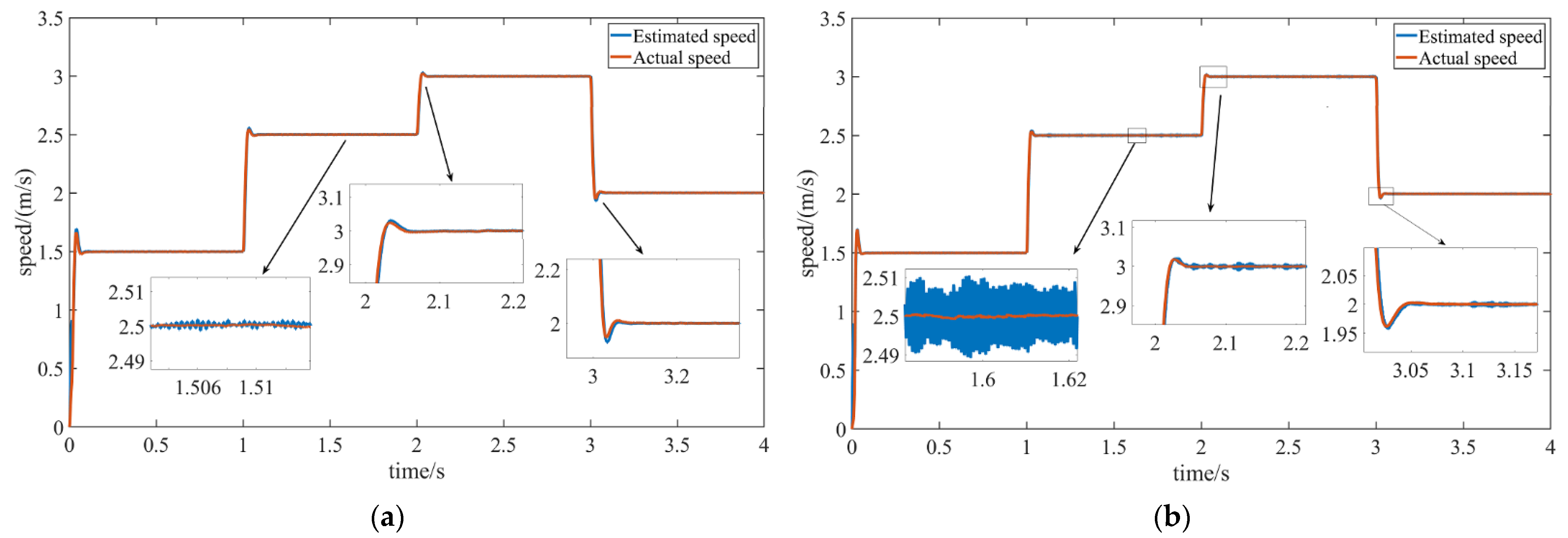
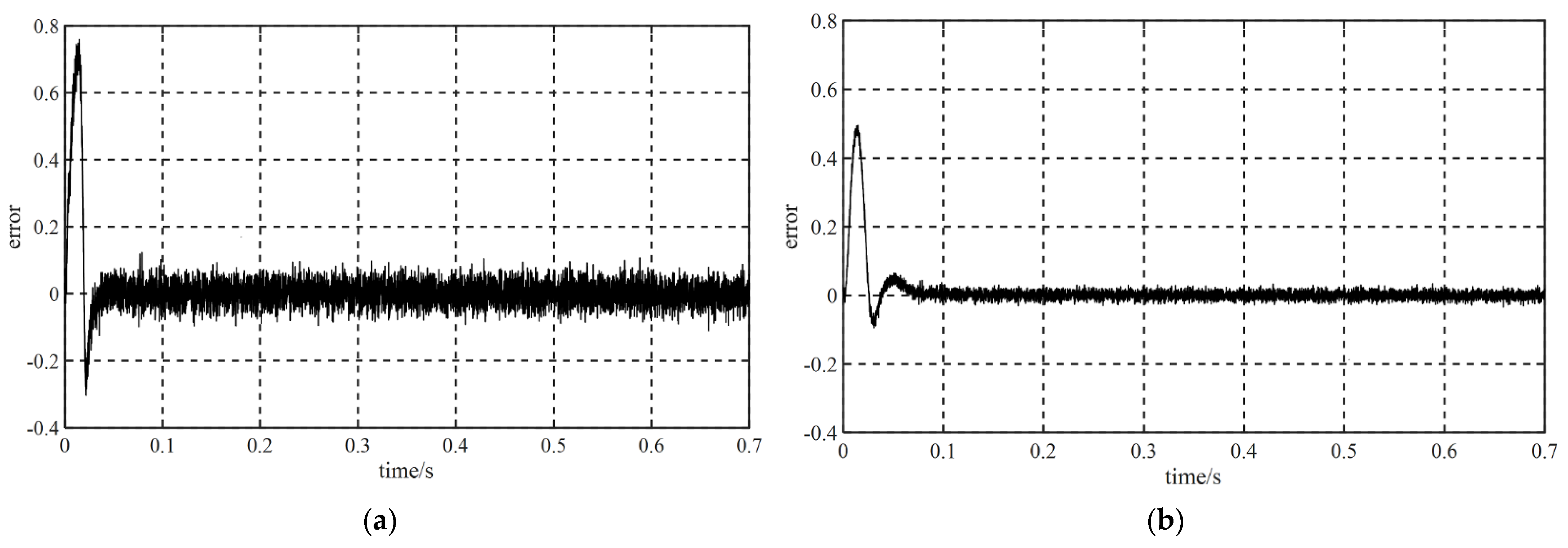
6.1.3. Comparison of Observation Effect between ST-SMO and Traditional SMO

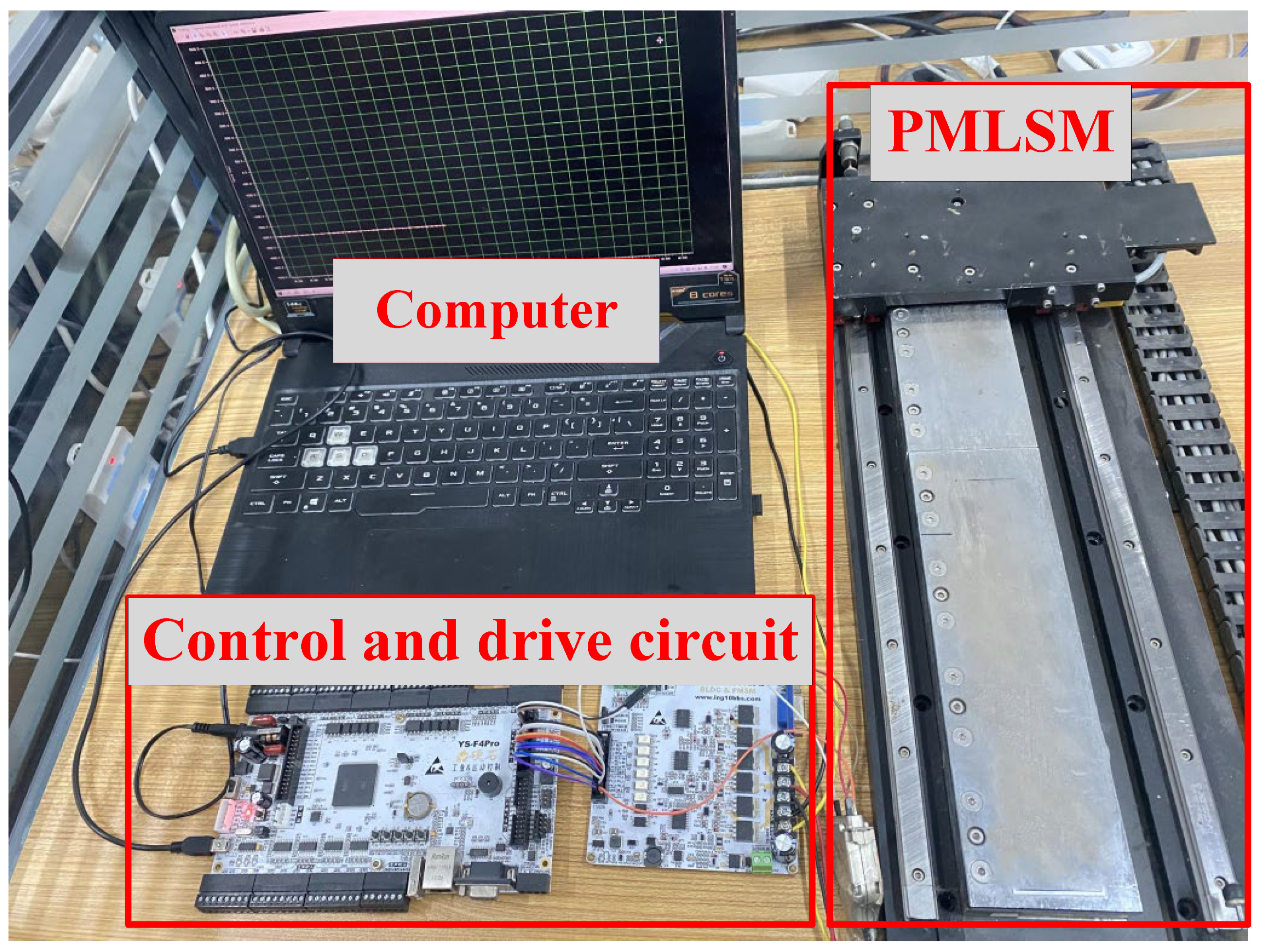
The above parts of the speed change and load change are simulations of the three controllers without adding observers. After verifying that the model-predicted speed and current integrated controller proposed in this paper has better control performance than the PI system and the SMC system, the ST-SMO and traditional SMO are used to compare the variable-speed operation on the basis of the integrated predictive control system. Figure 12a,b shows the comparison of the estimated speed to the actual speed of the control system after adding the ST-SMO and the traditional SMO. When the system changes speed, the stability of the traditional SMO system is poor, and the jitter amplitude is large. When the motor runs at the speed of 2.5 m/s, the jitter amplitude of the traditional SMO system is about 0.2 m/s. The ST-SMO system operates stably at various given speeds without obvious fluctuation, and the accuracy performance is greatly improved.

6.2. Experiment

The PMLSM experimental platform built in this paper is shown in Figure 13. The platform uses a TMS320F28335 chip to control the PMLSM. The mechanical sensor in the PMLSM is used for speed comparison and observer verification. The PMLSM parameters obtained in the experiment are consistent with the simulation results. The rated speed of the PMLSM used in this paper is 2 m/s, the rated thrust is 45 N, the rated current is 4 A, the rated voltage is 48 V, and the rated frequency is 5 KHz. During the experiment, the sampling time of the system is 500 μs, and the switching frequency is 5 KHz.

Compared with the ideal environment of simulation, the running environment in the experiment causes a significant increase in interference. The given speed of the control system is 1 m/s, and the given speed increases to 1.5 m/s at 0.4 s. Figure 14a shows the speed waveform of the PI system; Figure 14b shows the speed waveform of the SMC control system, and Figure 14c shows the speed waveform of the MPC system. In order to better analyze the speed waveforms of the three systems, the speed-overshoot and settling time of the 3 systems in the 2 steps of variable-speed movement are shown in Figure 15. By comparing the speed waveform obtained by the three operations in the experiment, the model predictive integrated control strategy involved in this paper has a better speed-regulation performance than both the PI system and the SMC system.

Figure 16 shows the detected current changes of the PI system, the SMC system, and the MPC system during the experiment, respectively. Figure 16 shows that the MPC system designed in this paper can adjust the current faster and make the motor speed reach the expected value. At the same time, the current jitter amplitude of the MPC system is smaller and more stable than that of the PI system and the SMC system.

We set the system speed to 1 m/s and add a load of 80 N at 0.4 s. Figure 17a is the speed waveform of the PI system, Figure 17b is the speed waveform of the SMC control system, and Figure 17c is the speed waveform of the MPC system. “Dynamic landing” refers to the magnitude of the speed fluctuation caused by the influence of the added load on the speed waveform of the system. In order to better analyze the velocity waveforms of the 3 systems, the dynamic landing and settling time of the 3 systems when the loads are increased are shown in Figure 18. By comparing the velocity waveforms obtained from the 3 operations, we can see that the MPC system in this paper has a faster settling time and smaller dynamic landing than either the PI system or the SMC system.

Figure 19 shows the current waveform changes of the MPC system, the PI system, and the SMC system after a sudden load is applied. After increasing the load, the current of the MPC system rises rapidly, increasing the thrust of the motor and resisting the impact of the load on the system. The PI system and the SMC system take a long time to bring the current to the expected level. Meanwhile, compared with those of the PI system and the SMC system, the current waveform of the MPC system is more stable, the jitter is smaller, and the response speed is faster.

The above experimental parts are the waveform results of the three controllers without adding an observer. The following is a comparison of the speed-tracking performance of a traditional SMO observer and the designed ST-SMO observer on the basis of the designed model-prediction integrated controller. Figure 20a,b shows the speed-tracking errors of the ST-SMO and the traditional SMO under the MPC-based system. Given a speed of 1 m/s, the chattering of the ST-SMO is lesser and more stable, and the chattering amplitude is about 0.025 m/s. The chattering of the traditional SMO is relatively large, and the chattering amplitude is about 0.1 m/s, which is 4 times that of the ST-SMO. The ST-SMO designed in this paper is more stable and demonstrates better tracking performance than does the traditional SMO.

7. Conclusions

To solve the problems of a PMLSM under variable speeds and loads, such as speed fluctuation, long adjustment times, and inevitable mechanical chattering, a PMLSM model predictive integrated control system based on an ST-SMO was designed. According to the dynamics and electrical equations of the PMLSM, an integrated speed and current controller based on an MPC was designed to replace the traditional PI control. Using an ST-SMO instead of a traditional SMO, the stability of system and the precision of the observer improve effectively. In the simulation and experiment, by comparing the designed MPC system with a PI system and an SMC system, under the condition of variable-speed movement and variable-load movement, the better control performance of the designed MPC system is reflected in three aspects: speed overshoot, dynamic landing, and settling time. The model predictive integrated controller designed in this paper integrates the speed loop and the current loop for control, and one only needs to adjust three parameters. Meanwhile, the sensorless control strategy is adopted on this basis, and the designed ST-SMO is added to cause the system to rid itself of its dependence on mechanical sensors to achieve the purpose of simplifying the system structure. The PMLSM system designed in this paper has better control performance and speed-tracking ability, which makes the running speed of the system more stable, and there is less current fluctuation than in a PI system, an SMC system, or an SMO system. The system designed in this paper has reference value for the design of PMLSM systems.

References

1. Cheng, H.; Sun, S.; Zhou, X.; Shao, D.; Mi, S.; Hu, Y. Sensorless DPCC of PMLSM Using SOGI-PLL-Based High-Order SMO With Cogging Force Feedforward Compensation. IEEE Trans. Transp. Electrif. 2022, 8, 1094–1104. [Google Scholar] [CrossRef]
2. Dong, F.; Zhao, J.; Zhao, J.; Song, J.; Chen, J.; Zheng, Z. Robust Optimization of PMLSM Based on a New Filled Function Algorithm with a Sigma Level Stability Convergence Criterion. IEEE Trans. Ind. Inform. 2021, 17, 4743–4754. [Google Scholar] [CrossRef]
3. Yang, R.; Li, L.; Wang, M.; Zhang, C. Force Ripple Compensation and Robust Predictive Current Control of PMLSM Using Augmented Generalized Proportional–Integral Observer. IEEE J. Emerg. Sel. Top. Power Electron. 2021, 9, 302–315. [Google Scholar] [CrossRef]
4. Zhao, J.; Mou, Q.; Zhu, C.; Chen, Z.; Li, J. Study on a Double-Sided Permanent-Magnet Linear Synchronous Motor With Reversed Slots. IEEE/ASME Trans. Mechatron. 2021, 26, 3–12. [Google Scholar] [CrossRef]
5. Yang, R.; Wang, M.; Li, L.; Wang, G.; Zhong, C. Robust Predictive Current Control of PMLSM With Extended State Modeling Based Kalman Filter: For Time-Varying Disturbance Rejection. IEEE Trans. Power Electron. 2020, 35, 2208–2221. [Google Scholar] [CrossRef]
6. Yongling, W.; Hong, L.; Xinda, S.; Baodong, C. Research on current harmonic suppression method of permanent magnet synchronous motor based on improved repetitive controller. Trans. Chin. Soc. Electr. Eng. 2019, 34, 2277–2286. [Google Scholar]
7. Niu, H.; Ma, Z.; Han, Y.; Chen, G.; Liao, Z.; Lin, G. Model Predictive Control with Common-Mode Voltage Minimization for a Three-level NPC Inverter PMLSM Drive System. In Proceedings of the 2021 13th International Symposium on Linear Drives for Industry Applications (LDIA), Wuhan, China, 1–3 July 2021; pp. 1–5. [Google Scholar]
8. ZMa, Z.; Sun, Y.; Zhao, Y.; Zhang, Z.; Lin, G. Dichotomy Solution Based Model Predictive Control for Permanent Magnet Linear Synchronous Motors. In Proceedings of the 2019 22nd International Conference on Electrical Machines and Systems (ICEMS), Harbin, China, 11–14 August 2019; pp. 1–5. [Google Scholar]
9. Ye, X.; Yang, Z.; Zhang, T. Modelling and performance analysis on a bearingless fixed-pole rotor induction motor. IET Electr. Power Appl. 2019, 13, 251–258. [Google Scholar] [CrossRef]
10. Zhang, H.; Li, H. Fast Commutation Error Compensation Method of Sensorless Control for MSCMG BLDC Motor With Nonideal Back EMF. IEEE Trans. Power Electron. 2021, 36, 8044–8054. [Google Scholar] [CrossRef]
11. Sarsembayev, B.; Suleimenov, K.; Do, T.D. High Order Disturbance Observer Based PI-PI Control System with Tracking Anti-Windup Technique for Improvement of Transient Performance of PMSM. IEEE Access 2021, 9, 66323–66334. [Google Scholar] [CrossRef]
12. Nguyen, A.T.; Rafaq, M.S.; Choi, H.H.; Jung, J.W. A Model Reference Adaptive Control Based Speed Controller for a Surface-Mounted Permanent Magnet Synchronous Motor Drive. IEEE Trans. Ind. Electron. 2018, 65, 9399–9409. [Google Scholar] [CrossRef]
13. Tang, Y.; Xu, W.; Liu, Y.; Dong, D. Dynamic Performance Enhancement Method Based on Improved Model Reference Adaptive System for SPMSM Sensorless Drives. IEEE Access 2021, 9, 135012–135023. [Google Scholar] [CrossRef]
14. Yang, C.; Ma, T.; Che, Z.; Zhou, L. An Adaptive-Gain Sliding Mode Observer for Sensorless Control of Permanent Magnet Linear Synchronous Motors. IEEE Access 2018, 6, 3469–3478. [Google Scholar] [CrossRef]
15. Zhang, X.; Li, Z. Sliding-Mode Observer-Based Mechanical Parameter Estimation for Permanent Magnet Synchronous Motor. IEEE Trans. Power Electron. 2016, 31, 5732–5745. [Google Scholar] [CrossRef]
16. Xu, W.; Junejo, A.K.; Tang, Y.; Shahab, M.; Habib, H.U.R.; Liu, Y.; Huang, S. Composite Speed Control of PMSM Drive System Based on Finite Time Sliding Mode Observer. IEEE Access 2021, 9, 151803–151813. [Google Scholar] [CrossRef]
17. Liu, Y.C.; Laghrouche, S.; Depernet, D.; Djerdir, A.; Cirrincione, M. Disturbance-Observer-Based Complementary Sliding-Mode Speed Control for PMSM Drives: A Super-Twisting Sliding-Mode Observer-Based Approach. IEEE J. Emerg. Sel. Top. Power Electron. 2021, 9, 5416–5428. [Google Scholar] [CrossRef]
18. Bıçak, A.; Gelen, A. Sensorless direct torque control based on seven-level torque hysteresis controller for five-phase IPMSM using a sliding-mode observer. Eng. Sci. Technol. 2021, 24, 1134–1143. [Google Scholar] [CrossRef]
19. Kumar, V.; Mohanty, S.R.; Kumar, S. Event Trigger Super Twisting Sliding Mode Control for DC Micro Grid With Matched/Unmatched Disturbance Observer. IEEE Trans. Smart Grid 2020, 11, 3837–3849. [Google Scholar] [CrossRef]
20. Li, Z.; Zhou, S.; Xiao, Y.; Wang, L. Sensorless Vector Control of Permanent Magnet Synchronous Linear Motor Based on Self-Adaptive Super-Twisting Sliding Mode Controller. IEEE Access 2019, 7, 44998–45011. [Google Scholar] [CrossRef]
21. Mao, S.; Tao, H.; Zheng, Z. Sensorless Control of Induction Motors Based on Fractional-Order Linear Super-Twisting Sliding Mode Observer with Flux Linkage Compensation. IEEE Access 2020, 8, 172308–172317. [Google Scholar]
22. Levant, A. Principles of 2-sliding mode design. Automatica 2007, 43, 576–586. [Google Scholar] [CrossRef] [Green Version]
Figure 1. Structure diagram of the PMLSM.
Energies 15 05504 g001
Figure 2. MPC system.
Energies 15 05504 g002
Figure 3. ST-SMO structure block diagram.
Energies 15 05504 g003
Figure 4. PLL structure block diagram.
Energies 15 05504 g004
Figure 5. Control system structure.
Energies 15 05504 g005
Figure 6. Comparison of variable-speed motion.
Energies 15 05504 g006
Figure 7. Comparison of the q-axis current waveforms of the three systems.
Energies 15 05504 g007
Figure 8. Comparison of operating speeds under variable loads.
Energies 15 05504 g008
Figure 9. Comparison of the current waveforms of the three systems.
Energies 15 05504 g009
Figure 10. Random loads added to the three systems.
Energies 15 05504 g010
Figure 11. Comparison of operating speeds under random loads.
Energies 15 05504 g011
Figure 12. Comparison of the tracking performance of two systems: (a) ST-SMO system; (b) traditional SMO system.
Energies 15 05504 g012
Figure 13. Experimental diagram.
Energies 15 05504 g013
Figure 14. Comparison of the tracking performance of the three systems: (a) PI system; (b) SMC system; and (c) MPC system.
Energies 15 05504 g014
Figure 15. Comparison of the speed-overshoot and settling times of the three controllers under speed variation: (a) Speed-overshoot and (b) Settling time.
Energies 15 05504 g015
Figure 16. Comparison of the current waveforms of the 3 systems under variable-speed motion: (a) PI system; (b) SMC system; and (c) MPC system.
Energies 15 05504 g016
Figure 17. Comparison of velocity waveforms of the 3 systems under sudden loads: (a) PI system; (b) SMC system; and (c) MPC system.
Energies 15 05504 g017
Figure 18. Comparison of the dynamic landing and the settling times of the three controllers under load variation: (a) Dynamic landing, and (b) Settling time.
Energies 15 05504 g018
Figure 19. Comparison of the current waveforms of the 3 systems under a sudden load: (a) PI system; (b) SMC system; and (c) MPC system.
Energies 15 05504 g019
Figure 20. Comparison of the speed-tracking errors of two systems: (a) Traditional SMO system and (b) ST-SMO system.
Energies 15 05504 g020