An Analysis of Thermal Comfort Models: Which One Is Suitable Model to Assess Thermal Reality in Brazil?

Abstract

The Predicted Mean Vote (PMV) has discrepancies in relation to the thermal reality of the environment; thus, adaptive models serve to improve this estimate. In this context, this research aimed to verify the performance of PMV and adaptive models under different conditions in Brazil from an analysis of variance and to further classify individuals into clusters according to their feelings of thermal comfort. Through ASHRAE’s Global II Thermal Comfort Database, users of offices and classrooms in Brasilia, Recife, Maceió, and Florianópolis were investigated. The results of ANOVA showed that the PMV model did not represent the thermal reality of any of the cities investigated, and the cluster analysis showed how most people felt thermally in relation to indoor environments.

1. Introduction

Globally, buildings consume about 40% of all the energy produced worldwide and a large part of it is used to promote comfort levels to indoor users [1]. To analyze indoor environmental conditions of thermal comfort, numerous models have been developed, but the most widely used is the PMV (Predicted Mean Vote), developed by Fanger in 1970. This model is relatively efficient; thus, there is a need to develop new models [2].

Thermal Comfort is indispensable for any environment [3] and indicates how thermally satisfied people are according to their state of mind [4]. Comfort studies can occur in residential spaces when there is temperature change at various points, different clothing, activities, or even when there are possibilities for adaptive actions in thermal environments [5]. Thermal environments directly influence the well-being [6], quality of life [7], health [8], and productivity [5] of people. Moreover, the assessment of thermal comfort in environments can contribute to the decrease in the use of ventilation, heating, and air-conditioning systems, consequently reducing energy consumption [9].

In their research, Cheung et al. [10] confirmed that Fanger’s PMV model contains an accuracy of only 34% in its results. With the possibility of improving the prediction of thermal comfort sensations, many adaptive models have come to be developed, such as: Nguyen, Singh, and Reiter [11]; Liping et al. [12]; Ruiz and Correa [13]; Gilani, Khan, and Ali [14]; Zhang et al. [15]. Several adaptive thermal comfort studies have been conducted in numerous environments and countries, such as in housing in Japan [16], educational buildings in Mexico [17], and office buildings in Spain [18] and in Brazil [19]. The adaptive thermal comfort model can more efficiently explain the existing discrepancies between predicted and actual thermal responses [20].

Together with the alternative models, several statistical methods have been applied to analyze thermal comfort, such as discriminant analysis [21], Bayesian statistics [22], Griffiths analysis [23], logistic regression [24], and structural equations [25]. Another relevant technique is the analysis of variance (ANOVA) that investigates the influences of some experimental conditions, errors, and significance of factors [26] and cluster analysis that classifies objects into homogeneous groups according to their level of similarity [27].

Some examples can be found in the literature, such as in the research of Lau, Chung, and Ren [28] who used analysis of variance (ANOVA) to determine whether weather variables and corresponding subjective perception were significantly different between Local Climate Zones (LCZs); Nduka et al. [29] who investigated the link between indoor environmental quality (IEQ) and symptoms of sick building syndrome (SBS); Sun et al. [30] who used cluster analysis in obtaining patterns of window opening duration in offices through a monitoring carried out by users; Piekut [31] who identified the clusters of households according to different energy consumption patterns.

In a recent study, Niza and Broday [32] verified through canonical discriminant functions that the PMV model did not contribute significantly to express the thermal sensation of people in the analyzed cities. Based on this context, this research aimed to verify the performance of the PMV and adaptive models under different conditions in Brazil from an analysis of variance and to classify individuals into clusters according to their feelings of thermal comfort.

In this perspective, we sought to fill this gap in the literature that refers to a comparative analysis between the PMV models based on data from Brazilian cities found in the ASHRAE Global Thermal Comfort Database II, the largest reference database in the area. Furthermore, the use of adaptive PMV models allows environment users to perform a better thermal comfort adjustment through more suitable clothing, ventilation, opening windows to save energy, among others [33]. Brazil was investigated for being a continental country with very diverse climates and regions; thus, the cities of Brasilia, Recife [34], Maceió [35], and Florianópolis [36] were analyzed.

2. Materials and Methods

2.1. Database

This research aimed to analyze the performance of alternative models to the PMV under different conditions in Brazil and to verify how individuals classify themselves into groups based on the highest level of similarity in relation to their thermal sensations. Through the application of alternative models to the PMV, the thermal sensations of individuals in the cities of Brasília, Recife, Maceió, and Florianópolis were obtained. The data applied in the formulas are available in the ASHRAE Global Thermal Comfort Database II, so the sample size could not be modified.

According to Földváry et al. [37], the database is composed of numerous field surveys, where these researchers have granted their data for any individual to make use of in new work, further enriching research in the area. The data available are:

• Basic identifiers: publication (citation), data contributor, year, season, climate, city, country, building type, and ventilation strategies used.
• Personal information of the individual: age, sex, weight, and height.
• Subjective information of thermal comfort: thermal sensation, thermal acceptability, thermal preference, air movement acceptability, air movement preference, thermal comfort, thermal insulation of clothing, metabolic rate, and humidity sensation.
• Instrumental measurements of thermal comfort: air temperature, operating temperature, radiant temperature, globe temperature, relative humidity, and air speed.
• Calculated indices: PMV, PPD, and standard effective temperature.
• Environmental control used: curtain, blinds, fan, window, door, heater, and monthly outside air temperature.

These variables change from researcher to researcher, but it is extremely necessary for the calculations of thermal comfort models: the presence of air temperature, mean radiant temperature, air speed, relative humidity, metabolic rate, and thermal insulation of clothing, with these being the most important variables to perform the analyses. Thus, it was possible to verify the compatibility of the alternative models to the PMV with the database.

The thermal comfort of individuals may vary according to the local climate; thus, studies of adaptive comfort become relevant to evaluate these differences related to acclimatization, culture, behavior, among other aspects [38].

2.2. Characterization of the Studied Area

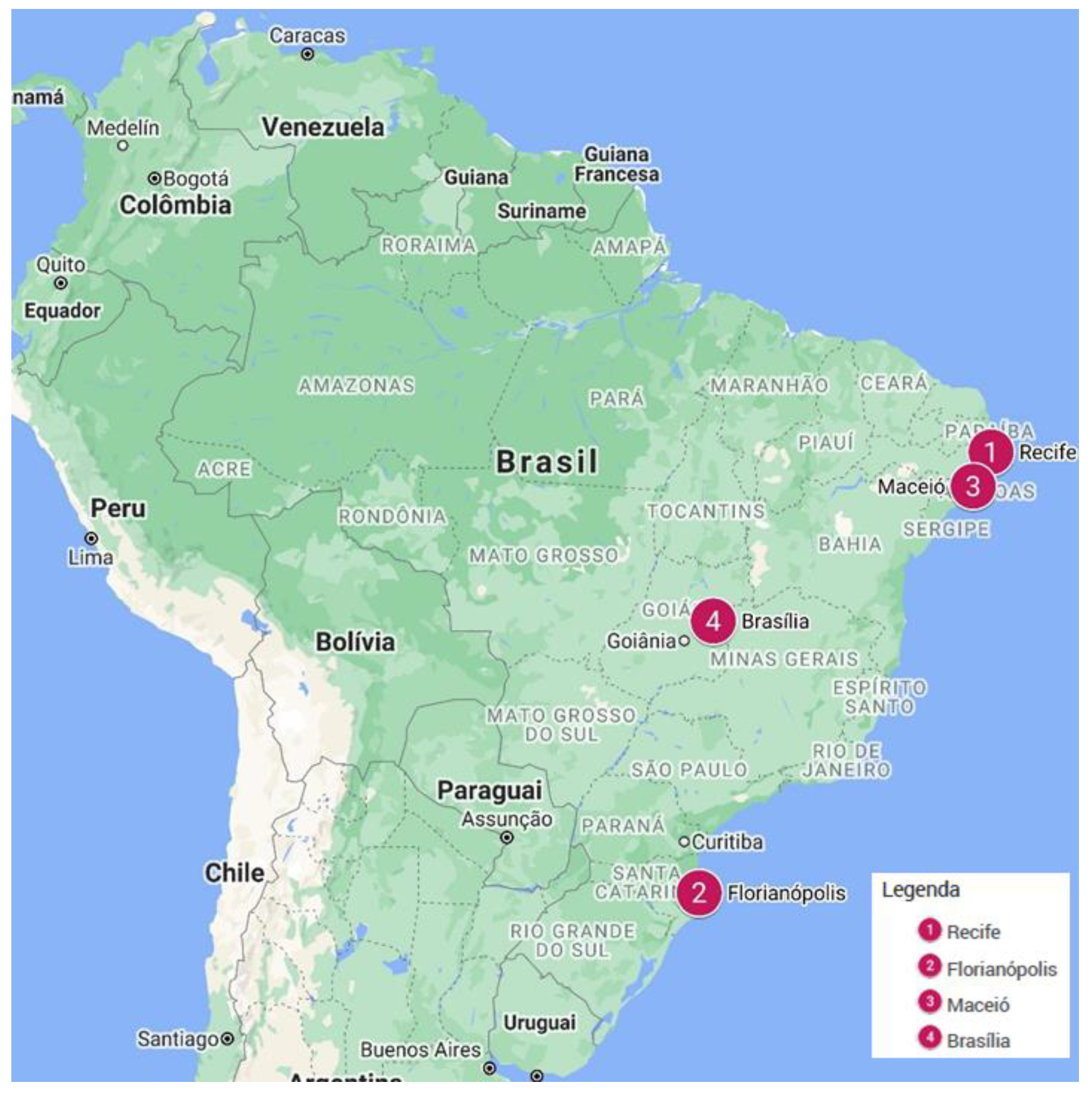
Through the availability of studies contained in the database, the cities of (1) Recife, (2) Florianópolis, (3) Maceió, and (4) Brasília were chosen for the analyses (Figure 1).

Among the countries available, Brazil was selected due to its continental dimension and its diverse climatic types in the regions, causing the presence of distinct thermal sensations experienced by the users. Through the Köppen–Geiger Classification, it was possible to verify the climatic zones of each region, with A for tropical, B for dry, C for temperate, D for continental, and E for polar [39]. Figure 2 shows the climate classifications, their respective colors, and legends. Climate types are influenced by locations, temperature, and local precipitation (Recife/Brasília-Aw, Florianópolis-Cfa, and Maceió-As).

2.3. Characterization of the Study

Figure 3 shows the information contained in the database, such as the data collection, year of collection, number of people that were studied by the authors, seasons of the year, building type, cooling strategies, age, gender, height, and weight of the individuals.

By joining the data, it was possible to obtain 6715 people participating in the field research, to combine the measurement of personal and environmental variables, and to report their thermal sensations and preferences.

2.4. Alternative Models Analyzed

Table 1. Alternative models of Thermal Comfort.

Ref.	Nomenclature Adopted in this Research	Climate Type	Models
[41]	PMVnew	Cfb	$D_{PMV-ASHRAE}=-4.03+0.00949t_{op}+0.00584\left(RH\%\right)+1.201\left(M. clo\right)+0.000838 t^2{}_{out}$
			$PM{V}_{new}=0.8 \left(PMV-D_{PMV-ASHARE}\right)$
[42]	aPMV	Cfa	$\mathrm{aPMV}=\frac{\mathit{PMV}}{1+0.293 \mathit{PMV}}$	$\mathrm{aPMV}=\frac{\mathit{PMV}}{1 - 0.125 \mathit{PMV}}$
[43]	PMVoo	Csb	${\mathit{PMV}}_n=-5.151+0.202 t+0{.553 P}_v$
[11]	PMVnsr	Af, Am, Aw, Cfa	$T_{\mathrm{comf}}=0{.341T}_{\mathrm{out}}+18.83$
[44]	PMVbrv	Csa, Cfa	$\mathit{PMV}=0{.2428t}_{\mathrm{op}} - 5.3562$
[45]	AdapPMV	Dwa	$Adaptative PMV model=\frac{PMV}{1+\left(-1.40\right)PMV}$
			$Adaptative PMV model=\frac{PMV}{1+\left(-5.74\right)PMV}$
[13]	IZA	Cfa	$\mathrm{IZA}=-0.9796+0{.0621t}_a - 0.3257v+0.0079\mathrm{HR}$
[46]	PMV*	Cfb	$PMV\ast =[0.303exp.\left(-0.036M\right)+0.028.L_{new}$
[47]	PMV2	Cfb, Csb	${\mathit{PMV}}_2=13.414 - 0.00003584(34 - t_a)+0.092.M.\left(5.87-p_a\right)-5.87\left(573-0.007\left[M-W\right]-p_a\right)-{\mathrm{0.53.10}}^{-8}.f_{cl}.\left[{\left(t_{cl\left(Newton\right)}+273\right)}^4-{\left(t_{rm}+273\right)}^4\right]-0.169f_{cl}.h_c.\left(t_{cl\left(Newton\right)}-t_a\right)$
[48]	PMVnew	Cfa	$PM{V}_{new}=\left(0.303e^{-0.036M}+0.28\right)\left\{M-W-0.0014M\left(34-t_a\right)-{\mathrm{3.96.10}}^{-8}{f}_{cl}\left[{\left(t_{cl}+273\right)}^4-{\left(t_{rm}+273\right)}^4\right]-f_{cl}{h}_c\left(t_{cl}-t_a\right)-{\mathrm{1.7.10}}^{-5}M\left(5867-P_v\right)-0.00305\left[5733-6.99\left(M-W\right)-P_v\right]-Q_{sw}\right\}$
[49]	ePMV	Cfa	$ePM{V}_p=e_{p}PMV$
[15]	PMVp,sv	Cfa	${\mathit{PMV}}_{p, \mathrm{SV}}=0{.0011T}_r{}^2+0{.4437v}_r{}^2 - 0{.1956T}_r{v}_r+0{.3073T}_r+4{.3290v}_r - 8.6710$

shows the alternative models used in this research. These models were previously selected according to the study by Niza and Broday [32].

2.5. Software Applied in the Research

Through the NVivo software, a word cloud was developed to represent the bibliometric network referring to the articles with the thermal comfort models used in this research; this way, the program contributes to increase the scientific credibility of the work, to verify the existing links between the studies, and to demonstrate the most frequent and important keywords in relation to the data.

The statistical analysis was performed in IBM SPSS Statistics software version 28. The analysis of variance (ANOVA) of the thermal sensations obtained between the traditional and alternative models allowed us to verify the performance under different climatic conditions in Brasília, Recife, Maceió, and Florianópolis. SPSS released a list with the models in order and named numerically. Next, Mauchly’s test of sphericity was used to validate the analysis of variance, where the p-value was analyzed under two hypotheses:

• H0: There is sphericity.
• H1: There is no sphericity.

For the between-subjects effects test, a further correction was required due to the lack of sphericity, and Greenhouse–Geiser, a more conservative correction, was used. Two hypotheses were considered:

• H3: Equality of group means.
• H4: At least one group mean is different.

Knowing that there is at least one different model is not enough, and it is necessary to investigate which model differs. To this end, the Bonferroni/pairwise post hoc test was used to compare model against model, verify the differences in means, and point out where this difference lies. The p-value is analyzed under two conditions, if:

• p-Value < 0.05: difference between the models.
• p-Value > 0.05: no difference between the models.

Possibly, some of the models that have similarities are not indicated in the calculations, so profile graphs were prepared.

In K-means Cluster analysis, the number of Clusters is determined by the researcher, and averages are calculated for grouping subjects [50]. The subjects are classified with the highest level of similarity between them. The results of the models were standardized to contribute uniformly to the results. Thus, the standardized variables are accompanied by Z. Next, the variations in the centers of the Clusters were obtained for each iteration until there was no more variation in the centroids. Through ANOVA, the variables that contributed most to the separation into clusters were identified, where they were classified according to their performance from the averages of each of the variables. The classification of clusters was carried out according to their performance in separating individuals into groups according to their thermal similarity:

• Positive average values for most variables: high performance/low risk.
• Negative average values for all or most variables: low performance/high senility risk.
• Average values close to zero: average performance/average senility risk.

Next, the distance matrix between the centroids and the number of individuals in each cluster is presented, and finally, its graphical representation.

3. Results

3.1. Bibliographic Networks

At first, a word cloud was prepared with the NVIVO software, from the articles presented in the research of Niza and Broday [32]; thus, the keywords of greatest occurrence in these studies were identified, putting in evidence the issues of greatest importance as presented in Figure 4.

The top ten words were: thermal (1267), pmv (929), comfort (764), model (656), temperature (643), air (427), buildings (356), average (342), adaptive (330), and data (326).

3.2. Analysis of Variance (ANOVA)

The results obtained by the models were submitted to SPSS to obtain the means and standard deviations of the calculated thermal sensation responses and the Thermal Sensation Voting (TSV) reported by the individuals in the database (

Table 2. Descriptive statistics.

	Brasília and Recife		Maceió		Florianópolis
Models	Mean	Standard Deviation	Mean	Standard Deviation	Mean	Standard Deviation
TSV (available in database)	0.67	0.87	0.40	0.94	0.05	0.88
PMV	−0.02	0.46	0.20	0.70	−0.51	0.57
PMVnew	-	-	0.11	0.38	−0.24	0.34
aPMV	−0.04	0.40	0.13	0.55	1.02	0.18
PMVoo	0.57	0.39	1.13	0.45	0.60	0.41
PMVnsr	−0.38	0.38	−0.19	0.57	−0.78	0.47
PMVbrv	0.55	0.47	1.23	0.55	0.60	0.50
AdapPMV	−0.27	0.36	−0.19	0.58	−0.28	0.63
IZA	0.96	0.14	1.13	0.12	0.97	0.15
PMV*	0.99	0.45	0.85	0.48	0.67	0.45
PMV2	0.78	0.71	0.57	0.77	0.28	0.72
PMVpsv	−0.22	0.60	0.20	0.69	−0.64	0.61
ePMV	0.41	0.82	0.24	0.60	−0.08	0.18
PMVnew2	−1.50	1.00	−0.004	0.07	−0.15	0.06

).

Other models were also selected for testing, but many of them were incompatible with the database. The model by Humphreys and Nicol [41] was not applied to the cities of Brasília and Recife, due to incompatibility with the database, as it required the external air temperature (t_out). The SPSS software numerically ordered the models, as shown in Figure 5.

Mauchly’s sphericity was used to validate the analysis of variance, where equalities were put to treatment (

Table 3. Mauchly’s test of sphericity.

	W de Mauchly	df	p-Values
Brasília and Recife	0.001	77	<0.001
Maceió	0.001	77	<0.001
Florianópolis	0.001	90	<0.001

df = degree of freedom.

). If sphericity is violated, the variance calculations may be distorted, causing an invalid result [51]. The p-values found in the results were less than the significance of 0.05, showing evidence that there was no sphericity [52], so H₁ was accepted. The degree of freedom was used to estimate the variance [53].

In the between-subjects effects test (

Table 4. Between-subjects effects test.

Origin		Type III Sum of Squares	df	Mean Square	F	p-Value
Brasília and Recife	Epsilon (Greenhouse–Geiser)	298.16	2.38	125.05	121.73	<0.001
Maceió		5077.80	2.92	1736.42	2328.04	<0.001
Florianópolis		22,728.43	3.22	7056.96	10,428.31	<0.001
Brasília and Recife	Error (models)	122.47	119.22	1.027
Maceió		3553.09	4763.67	0.75
Florianópolis		10,969.39	16,209.83	0.68

F = F-statistic; df = degree of freedom.

), there was no presence of sphericity, so the Greenhouse–Geiser correction was performed [54]. The p-value was less than 0.05; thus, the alternative hypothesis (H₁) was accepted, where there was at least one different thermal comfort model.

One-way repeated measures ANOVA was performed to show the presence of a significant effect on the factor with p-value < 0.05 [55], that is, showing the effect of the models on the TSV (thermal sensation vote): (F (2.38; 119.22) = 121.73, p-value < 0.001) for Brasília and Recife; (F (2.92; 4763.67) = 2328.04, p-value < 0.001) for Maceió; (F (3.22; 16,209.83) = 10,428.31, p-value < 0.001) for Florianópolis.

By Bonferroni’s post hoc test, Brasília and Recife had the PMVoo, PMVbrv, and ePMV models closest to TSV; for Maceió and Florianópolis, no model was resembled. Through this analysis, it was possible to perform pairwise comparisons between the models [56]. However, some similarities between the models may not be indicated in the calculations. Figure 6 shows the profile graphs for better visualization of the closeness of the models to the TSV, where each number on the horizontal axis represents the models used in this research, as presented in Figure 5. All points on the graphs in the same direction horizontally represent the models that most closely resemble the TSV.

Through the Bonferroni post hoc test, only model 13 (PMVnew2) was unlike any other model for Brasília and Recife; for the other models, there was at least one similarity. However, the profile graph and the averages of the thermal sensations were combined for the continuity of the analysis because the Bonferroni post hoc test did not show similar models to the TSV for the cities of Maceió and Florianópolis.

Thus, for Brasília and Recife, the model that best represented these cities was the PMVoo (4) of Orosa and Oliveira [43], with an average difference closer to the thermal sensation votes (TSV), with only a 0.10 difference from reality. In the Köppen–Geiger Classification, both are in tropical climate regions (A). This model was developed under temperate climates (C); even with climatic incompatibility, it adapted very well to data from cities as the authors developed it precisely for office environments.

In Maceió, through the profile graph, it was seen that the model that most closely matched the TSV was the PMV2 (11) developed by Broday et al. [47], with an average difference of only 0.16 with the thermal sensation votes. Its location is in a temperate (C) climate region, and this model was developed for sites with that same climate group, thus strongly influencing model performance.

Through the profile plot, the model that best represented Florianópolis was the ePMV (13) by Zhang and Lin [49], with an average difference of only 0.03 from the thermal sensation votes. Florianópolis is in a region of tropical climates (A), and the model was developed under temperate climates (C); thus, even with the presence of climatic incompatibility, the model behaved very well with the data; moreover, the authors validated their model in buildings with air-conditioning and natural ventilation, as is the case of classrooms/mixed-mode, office/mixed-mode, and office/air-conditioning in Florianópolis.

3.3. Cluster Analysis

The variation of the center of the clusters in each iteration is presented in

Table 5. Variation in the center of the clusters in each iteration.

Iteration (Brasília and Recife)	1	2	3	Iteration (Maceió)	1	2	3	Iteration (Florianópolis)	1	2	3
1	2.72	3.78	4.60	1	5.35	6.42	9.37	1	9.31	8.91	7.10
2	1.14	0.26	0.49	2	1.52	0.55	0.25	2	0.30	0.42	1.48
3	0.29	0.13	0.31	3	4.05	0.25	0.14	3	0.17	0.27	2.28
4	0.31	0.12	0.26	4	0.00	0.11	0.06	4	0.23	0.12	0.95
5	0.00	0.00	0.00	5	0.00	0.04	0.02	5	0.24	0.03	0.55
				6	0.00	0.01	0.01	6	0.19	0.08	0.26
				7	0.00	0.00	0.00	7	0.14	0.09	0.15
								8	0.12	0.08	0.11
								9	0.08	0.07	0.07
								10	0.08	0.06	0.06

, where Brasília and Recife have a minimum distance of 7.30 between the initial centers, Maceió with 13.98, and Florianópolis with 18.40. When there is no more significant variation in the centroids of each cluster, the algorithm will terminate.

The ANOVA is presented in

Table 6. ANOVA.

ANOVA
Brasília and Recife	Cluster	df	Error	df	F.	p-Value
	Mean Square		Mean Square
Zscore (TSV)	14.27	2	0.45	48	31.90	<0.001
Zscore (PMV)	17.08	2	0.33	48	51.73	<0.001
Zscore (aPMV)	17.26	2	0.32	48	53.56	<0.001
Zscore (PMVoo)	19.85	2	0.22	48	92.40	<0.001
Zscore (PMVnsr)	17.08	2	0.33	48	51.73	<0.001
Zscore (PMVbrv)	19.85	2	0.22	48	92.40	<0.001
Zscore: Adap PMV	0.13	2	1.04	48	0.12	0.884
Zscore (IZA)	15.47	2	0.40	48	38.97	<0.001
Zscore: PMV*	14.27	2	0,447	48	31.89	<0.001
Zscore (PMV2)	14.27	2	0,447	48	31.89	<0.001
Zscore: PMVp,sv	20.03	2	0,207	48	96.61	<0.001
Zscore (ePMV)	12.18	2	0,534	48	22.81	<0.001
Zscore (PMVnew2)	14.93	2	0.42	48	35.59	<0.001
Maceió	Cluster	df	Error	df	F.	p-Value
	Mean Square		Mean Square
Zscore (TSV)	259.58	2	0.68	1627	380.53	<0.001
Zscore (PMV)	509.96	2	0.37	1627	1362.25	<0.001
Zscore (PMVnew)	429.58	2	0.47	1627	907.89	<0.001
Zscore (aPMV)	500.46	2	0.39	1627	1296.41	<0.001
Zscore (PMVoo)	583.06	2	0.28	1627	2049.47	<0.001
Zscore (PMVnsr)	509.96	2	0.37	1627	1362.25	<0.001
Zscore (PMVbrv)	583.06	2	0.28	1627	2049.47	<0.001
Zscore: Adap PMV	472.92	2	0.42	1627	1126.32	<0.001
Zscore (IZA)	561.03	2	0.31	1627	1800.59	<0.001
Zscore: PMV*	259.58	2	0.68	1627	380.53	<0.001
Zscore (PMV2)	259.58	2	0.68	1627	380.53	<0.001
Zscore: PMVp,sv	591.73	2	0.27	1627	2160.84	<0.001
Zscore (ePMV)	396.55	2	0.51	1627	771.83	<0.001
Zscore (PMVnew2)	533.00	2	0.35	1627	1540.28	<0.001
Florianópolis	Cluster	df	Error	df	F.	p-Value
	Mean Square		Mean Square
Zscore (TSV)	746.19	2	0.70	5031	1059.98	<0.001
Zscore (PMV)	1378.34	2	0.45	5031	3045.02	<0.001
Zscore (PMVnew)	1252.25	2	0.50	5031	2490.78	<0.001
Zscore (aPMV)	496.72	2	0.80	5031	618.53	<0.001
Zscore (PMVoo)	1334.14	2	0.47	5031	2837.52	<0.001
Zscore (PMVnsr)	1378.34	2	0.45	5031	3045.02	<0.001
Zscore (PMVbrv)	1334.14	2	0.47	5031	2837.52	<0.001
Zscore: Adap PMV	73.22	2	0.97	5031	75.37	<0.001
Zscore (IZA)	1274.67	2	0.49	5031	2580.97	<0.001
Zscore: PMV*	746.19	2	0.70	5031	1059.98	<0.001
Zscore (PMV2)	746.19	2	0.70	5031	1059.98	<0.001
Zscore: PMVp,sv	1415.30	2	0.44	5031	3231.82	<0.001
Zscore (ePMV)	483.05	2	0.81	5031	597.57	<0.001
Zscore (PMVnew2)	1512.35	2	0.40	5031	3786.81	<0.001

F = F-statistic; df = degree of freedom.

, where the variables highlighted in green are those with the best discrimination between the Brasília and Recife clusters (PMVp,sv—96.61, PMVbrv—92.40, and PMVoo—92.40); Maceió (PMVp,sv—2160.84, PMVbrv—2049.47, and PMVoo—2049.47); Florianópolis (PMVnew2—3786.81, PMVp,sv—3231.82, PMVnsr—3045.02, and PMV—3045.02). Highlighted in red are the variables that present the least discrimination between the clusters of Brasília and Recife (Adap PMV—0.12); Maceió (TSV—380.53, PMV*—380.53, and PMV2—380.53); Florianópolis (Adap PMV—75.37). Through these F values, it is possible to verify how significant the variables are for the realization of the separation into groups [57]; that is, the variables with better discrimination have a higher level of similarity for the completion of the clusters and the variables with lower discrimination are the ones that contribute less.

F-Tests are only used for descriptive purposes, as the clusters are chosen to verify the existing variability between and within groups, that is, the higher the value of F is, the greater the contribution of the variable to the definition of the groups. In

Table 7. Final group centers.

Clusters
Models	Brasília and Recife			Maceió			Florianópolis
	1	2	3	1	2	3	1	2	3
Zscore (TSV)	1.34	−0.66	−0.08	0.28	0.76	−0.42	−0.05	−0.50	1.02
Zscore (PMV)	1.30	−0.87	0.15	−0.05	1.07	−0.59	0.19	−0.87	1.15
Zscore (PMVnew)	-	-	-	−0.17	0.98	−0.54	0.18	−0.83	1.10
Zscore (aPMV)	1.27	−0.89	0.19	0.06	1.06	0.58	0.49	−0.47	−0.27
Zscore (PMVoo)	1.48	−0.88	0.07	0.34	1.14	−0.63	0.12	−0.82	1.20
Zscore (PMVnsr)	1.30	−0.87	0.15	−0.05	1.07	−0.59	0.19	−0.88	1.15
Zscore (PMVbrv)	1.48	−0.88	0.07	0.34	1.14	−0.63	0.12	−0.82	1.20
Zscore: Adap PMV	−0.03	0.09	−0.07	12.53	−0.04	−0.05	0.01	−0.18	0.30
Zscore (IZA)	1.36	−0.73	−0.02	0.31	1.12	−0.61	0.22	−0.86	1.06
Zscore: PMV*	1.34	−0.66	−0.08	0.28	0.76	−0.42	−0.05	−0.50	1.02
Zscore (PMV2)	1.34	−0.66	−0.08	0.28	0.76	−0.42	−0.05	−0.50	1.02
Zscore: PMVp,sv	1.11	−1.06	0.45	0.25	1.15	−0.63	0.12	−0.84	1.24
Zscore (ePMV)	1.27	−0.55	−0.15	−0.31	0.94	−0.52	0.16	−0.55	0.62
Zscore (PMVnew2)	0.15	0.82	−0.90	0.03	1.09	−0.60	0.15	−0.88	1.26

, it is possible to identify the averages for the variables in each of the clusters created.

With the values found in the centers of the final groups, it is possible to classify the clusters according to their performance, as follows:

• Brasília and Recife: cluster 1—high performance/low risk, cluster 2—low performance/high senility risk, and cluster 3—medium performance/medium senility risk;
• Maceió: cluster 1—medium performance/medium senility risk, cluster 2—high performance/low risk, and cluster 3—low performance/high senility risk;
• Florianópolis: cluster 1—medium performance/medium senility risk, cluster 2—low performance/high senility risk, and cluster 3—high performance/low senility risk.

Table 8. Matrix of distances between cluster centers.

	Distance Matrix
Cluster (Brasília and Recife)	1	2	3	Cluster (Maceió)	1	2	3	Cluster (Florianópolis)	1	2	3
1		7.08	4.39	1		13.00	12.84	1		3.21	3.54
2	7.08		3.47	2	13.00		5.67	2	3.21		6.43
3	4.39	3.47		3	12.84	5.67		3	3.54	6.43

contains the distance matrix between the centroids of the clusters.

The number of cases (individuals) in each cluster is shown in

Table 9. Number of cases in each cluster.

Cluster	Brasília and Recife	Maceió	Florianópolis
1	11	6	2258
2	20	575	1787
3	20	1049	989
Total	51	1630	5034

.

Next, Figure 7 represents the centers of the final clusters contained in Table 7 with the averages for the variables in each cluster created.

For Brasília and Recife, clusters 2 and 3 had the same number of people feeling slightly cool and slightly warm, respectively. In Maceió, cluster 3 had the highest number of people who felt slightly cool and, for this same city, there was an outlier in the variable AdapPMV present in cluster 1. In Florianópolis, the number of people was predominant in cluster 1, where the majority voted for thermal neutrality.

4. Discussion

One-way repeated measures ANOVA exposes differences that are statistically significant between groups (p-value < 0.05) [58]. Therefore, this statistical method contributed to verifying statistical differences between the PMV and its alternative models when applied under different climatic and environmental conditions. However, Mauchly’s test of sphericity was performed to confirm whether there was no equality between the models. However, it only proves a difference between the models but does not indicate exactly where this difference lies. This difference was investigated by the Bonferroni post hoc test, where a model-to-model comparison was made for comparative purposes [59] so that it is possible to find out which model best represented the thermal conditions of each city. Even after performing the test, it is possible that some models that resemble the thermal reality are not among the results found in the calculations, so with the profile graph, it became more visual to identify these similarities through the proximities between the TSV and the performance of the models themselves.

By performing the analysis of variance, the fact highlighted in the research of Cheung et al. [10] was confirmed, where it was found that the Fanger model presented only a 34% accuracy in its performance. Thus, the PMV had results that did not match the thermal realities found for the four Brazilian cities. Thus, for Brasília and Recife, the ‘PMVoo’ model of Orosa and Oliveira [43] presented the lowest mean difference between model results and thermal sensation votes at 0.10; for Maceió, it was the ‘PMV2’ model of Broday et al. [47] with 0.16; for Florianópolis, it was the ‘ePMV’ model of Zhang and Lin [49] with 0.03. In the profile graphs, all the points above the TSV represent the models that were overestimated, and the points below represent the models that underestimated the thermal sensation. In agreement with these results, Niza and Broday [32] developed canonical discriminant functions that proved that the adaptive models were more relevant than the PMV.

Knowing the model that best suits a particular condition makes it possible to understand how the users of the environment feel. Thus, it becomes easier to propose better thermal requirements for buildings, offer ventilation strategies, and even contribute to the execution of future construction projects. Another circumstance to be highlighted is the great usability of the analysis of variance in thermal comfort.

Lam, Loughnan, and Tapper [60] studied outdoor thermal comfort in Australia’s Royal Botanic Garden (RBG) during the summer, evaluating residents’ and tourists’ perceptions. Through the analysis, they investigated the differences in thermal perception between these two audiences to bring improvements to the garden’s design, making the site increasingly attractive for tours, and attracting several potential foreign visitors. Another application of this analysis was found in Kwong et al. [61]. They tested the statistical differences in average temperatures between local climate zones in the Metropolitan Region of Toulouse (France) under hot and dry summer conditions. Thus, this analysis’ broad applicability for indoor and outdoor environments is noted, in addition to health benefits and the ability to make tourist spots increasingly attractive.

Following this research, Kiki et al. [62] sought adaptive models capable of representing the thermal conditions of buildings in Benin, a country in West Africa, which, as with Brazil, has a tropical climate. In the same way that using thermal comfort studies to reduce energy losses is highlighted, it also emphasizes the search for comfort standards for users. In these air-conditioned buildings located in hot and humid regions, the adaptive models with the best performances were by López-Pérez, Flores-Prieto, and Ríos-Rojas [17] and Indraganti et al. [63]; thus, as mentioned before, the models’ performances may vary from environment to environment. Therefore, the model considered optimal for Benin may not perform well when applied to Brazil and vice versa.

Next, through cluster analysis, it was possible to divide the data of thermal sensations obtained by the models into k clusters, where everyone was assigned to a group [64], i.e., each person should be assigned to only one cluster according to their thermal sensation, so all those who have thermal similarities will be in the same group. Nam et al. [65] cited that if, by chance, an object belongs to a cluster, it becomes impossible to transfer it to another; thus, if there are outliers, they cannot be removed, as was the case of the outlier found in cluster 1 of Maceió that contained well-dispersed thermal sensations that benefited for the variable ‘AdapPMV’ to present a higher thermal sensation than the one present in the 7-point scale of ASHRAE.

Throughout the iterations, the centroids are modified until there is no significant variation between the averages, and thus, each element is allocated to only one cluster. Through the clusters and the similarities, it is possible to investigate how most people felt to analyze these environments more pointedly according to these aspects and consequently meet the needs of most users by improving them thermally.

Among the studies found, Asumadu-Sakyi et al. [66] identified the patterns in indoor temperature for weekdays and weekends in homes in mid-season periods and homes with air conditioning in hot and cold seasons. The author also mentioned that for future works, several pieces of data can be incremented, such as socioeconomic data of the users, types of walls of the buildings, and floor insulation, that can contribute to the understanding of the results both for Brisbane in Australia and Florianópolis in Brazil that are under the same climate for being located at the same latitude. For the application of adaptive strategies, Bienvenido-Huertas et al. [9] considered temperature records from the 20th century until 2019 in buildings in southern Spain. Hence, cluster analysis has a versatile application in numerous areas, enabling the union of elements with common characteristics in clusters.

According to Wu et al. [67], much research in thermal comfort focused on building energy savings ends up neglecting human adaptation, and this factor is one of the main factors for maintaining thermal comfort. Therefore, investigating of how individuals feel, adaptive behavior, and strategies used in the environment become increasingly necessary to consider in developing adaptive models. Furthermore, Altan and Ozarisoy [68] emphasized that information about the thermal comfort requirements under different climate types can contribute to the suggestion of appropriate environmental and design solutions, providing a comfortable and satisfactory thermal environment. In summary, both statistical analyses were highly relevant to thermal comfort, presenting new perspectives, possibilities, and directions for the progress of studies and scientific research.

5. Conclusions

In the analysis of variance, it was possible to test the PMV and alternative models to see which would perform best under different conditions in Brazil using the ASHRAE Global Thermal Comfort Database II. Thus, for Brasília and Recife, the PMVoo model by Orosa and Oliveira [43] showed the lowest mean difference between model results and thermal sensation votes at 0.10; for Maceió, it was the PMV2 model by Broday et al. [47] with 0.16; for Florianópolis, it was the ePMV model by Zhang and Lin [49] with 0.03. With the results, it was confirmed that alternative models could have greater accuracy than the traditional PMV model, and the development of these new models could become increasingly more usual and effective in the search for greater precision about the thermal reality found in environments, in addition to their contribution to energy efficiency, productivity, health, and well-being. In addition, it highlights that their particularities mean that the models can present different performances under numerous regions.

Through cluster analysis, individuals were classified based on their similarities in the thermal sensation votes, identifying homogeneity in the data. Thus, in Brasília and Recife, the second and third clusters were responsible for grouping most people, with 20 people in each cluster who felt slightly warm and slightly cool, respectively. For Maceió, most people were allocated to the last cluster, with 1049 people who felt slightly cool; for Florianópolis, 2258 people were in the largest cluster where they felt slightly warm. Through the creation of the clusters, it became understandable how most people felt thermally through their level of thermal similarity. These aspects can contribute to identifying the needs of indoor users.

The size of the samples was one of the limitations found, where they presented very distinct sizes between cities that may have influenced the results. If there were more individual thermal responses, the approximation to reality would be better. It is suggested for future works the development of an analysis of thermal comfort for the southeast region, the most economically developed area in Brazil, and the north of the country, a region with high rainfall rates and a large amount of relative humidity, both of which directly influence the thermal sensation. In ASHRAE’s database, only these two Brazilian regions have not yet been included in the analyses. Thus, all the proposed objectives were achieved, presenting the thermal comfort models with greater adequacy to the cities and the distribution of individuals in groups according to the level of thermal similarity.

References

1. Ngarambe, J.; Yun, G.Y.; Santamouris, M. The use of artificial intelligence (AI) methods in the prediction of thermal comfort in buildings: Energy implications of AI-based thermal comfort controls. Energy Build. 2020, 211, 109807. [Google Scholar] [CrossRef]
2. Van Hoof, J. Forty years of Fanger’s model of thermal comfort: Comfort for all? Indoor Air 2008, 18, 182–201. [Google Scholar] [CrossRef] [PubMed]
3. Karahan, A.; Ertürk, E.F.; Ugurlu, Z.; Ünlü, H.; Akovali, N.; Tepe, A.; Elbas, N.O. Factors Affecting the Thermal Comfort of Perioperative Personnel in the OR. AORN J. 2020, 111, 333–344. [Google Scholar] [CrossRef] [PubMed]
4. Ravindra, K.; Argawal, N.; Mor, S. Assessment of thermal comfort parameters in various car models and mitigation strategies for extreme heat-health risks in the tropical climate. J. Environ. Manag. 2020, 267, 110655. [Google Scholar] [CrossRef] [PubMed]
5. Zomorodian, Z.S.; Tahsildoost, M.; Hafezi, M. Thermal comfort in educational buildings: A review article. Renew. Sust. Energy Rev. 2016, 59, 895–906. [Google Scholar] [CrossRef]
6. Rohde, L.; Larsen, T.S.; Jensen, R.L.; Larsen, O.K. Framing holistic indoor environment: Definitions of comfort, health and well-being. Indoor Built Environ. 2020, 29, 118–136. [Google Scholar] [CrossRef]
7. Mijani, N.; Alavipanah, S.K.; Hamzeh, S.; Firozjaei, M.K.; Arsanjani, J.J. Modeling thermal comfort in different condition of mind using satellite images: An Ordered Weighted Averaging approach and a case study. Ecol. Indic. 2019, 104, 1–12. [Google Scholar] [CrossRef]
8. Van Lichtenbelt, W.; Hanssen, M.; Pallubinsky, H.; Kingma, B.; Schellen, L. Healthy excursions outside the thermal comfort zone. Build. Res. Inf. 2017, 45, 819–827. [Google Scholar] [CrossRef] [Green Version]
9. Bienvenido-Huertas, D.; Rubio-Bellido, C.; Farinha, F.; Oliveira, M.J.; Pérez-Ordóñez, J.L. Evaluating the potential of adaptive comfort approach using historic data to reduce energy consumption in buildings in Southern Spain. Build. Environ. 2020, 185, 107313. [Google Scholar] [CrossRef]
10. Cheung, T.; Schiavon, S.; Parkinson, T.; Li, P.; Brager, G. Analysis of the accuracy on PMV—PPD model using the ASHRAE Global Thermal Comfort Database II. Build. Environ. 2019, 153, 215–217. [Google Scholar] [CrossRef] [Green Version]
11. Nguyen, A.T.; Singh, M.K.; Reiter, S. An adaptive thermal comfort model for hot humid South-East Asia. Build. Environ. 2012, 56, 291–300. [Google Scholar] [CrossRef] [Green Version]
12. Liping, P.; Yingjie, W.; Meng, L.; Helin, Z.; Jun, W. Method to predicting optimal cabin operative temperature for civil aircraft. Build. Environ. 2013, 69, 160–170. [Google Scholar] [CrossRef]
13. Ruiz, M.A.; Correa, E.N. Adaptive model for outdoor thermal comfort assessment in an Oasis city of arid climate. Build. Environ. 2015, 85, 40–51. [Google Scholar] [CrossRef]
14. Gilani, S.I.-U.; Khan, M.H.; Ali, M. Revisiting Fanger’s thermal comfort model using mean blood pressure as a bio-marker: An experimental investigation. Appl. Therm. Eng. 2016, 109, 35–43. [Google Scholar] [CrossRef]
15. Zhang, S.; Cheng, Y.; Oladokun, M.O.; Wu, Y.; Lin, Z. Improving predicted mean vote with inversely determined metabolic rate. Sustain. Cities Soc. 2020, 53, 101870. [Google Scholar] [CrossRef]
16. Rijal, H.B.; Humphreys, M.A.; Nicol, J.F. Adaptive model and the adaptive mechanisms for thermal comfort in Japanese dwellings. Energy Build. 2019, 202, 109371. [Google Scholar] [CrossRef]
17. López-Pérez, L.A.; Flores-Prieto, J.J.; Ríos-Rojas, C. Adaptive thermal comfort model for educational buildings in a hot-humid climate. Build. Environ. 2019, 150, 181–194. [Google Scholar] [CrossRef]
18. Barbadilla-Martín, E.; Lissén, J.M.S.; Martín, J.G.; Aparicio-Ruiz, P.; Brotas, L. Field study on adaptive thermal comfort in mixed mode office buildings in southwestern area of Spain. Build. Environ. 2017, 123, 163–175. [Google Scholar] [CrossRef]
19. Rupp, R.F.; De Dear, R.; Ghisi, E. Field study of mixed-mode office buildings in Southern Brazil using an adaptive thermal comfort framework. Energy Build. 2018, 158, 1475–1486. [Google Scholar] [CrossRef]
20. Toe, D.H.C.; Kubota, T. Development of an adaptive thermal comfort equation for naturally ventilated buildings in hot–humid climates using ASHRAE RP-884 database. Front. Archit. Res. 2013, 2, 278–291. [Google Scholar] [CrossRef] [Green Version]
21. Gładyszewska-Fiedoruk, K.; Sulewska, M.J. Thermal Comfort Evaluation Using Linear Discriminant Analysis (LDA) and Artificial Neural Networks (ANNs). Energies 2020, 13, 538. [Google Scholar] [CrossRef] [Green Version]
22. Benito, P.I.; Sebastián, M.A.; González-Gaya, C. Study and Application of Industrial Thermal Comfort Parameters by Using Bayesian Inference Techniques. Appl. Sci. 2021, 11, 11979. [Google Scholar] [CrossRef]
23. Tewari, P.; Mathur, S.; Mathur, J.; Kumar, S.; Loftness, V. Field study on indoor thermal comfort of office buildings using evaporative cooling in the composite climate of India. Energy Build. 2019, 199, 145–163. [Google Scholar] [CrossRef]
24. Ji, Y.; Wang, Z. Thermal adaptations and logistic regression analysis of thermal comfort in severe cold area based on two case studies. Energy Build. 2019, 205, 109560. [Google Scholar] [CrossRef]
25. Muñoz, J.S.; Kelly, M.T.; Flores-Alés, V.; Caamaño-Carrillo, C. Recognizing the effect of the thermal environment on self-perceived productivity in offices: A structural equation modeling perspective. Build. Environ. 2022, 210, 108696. [Google Scholar] [CrossRef]
26. Huang, X.; Zhang, Q.; Tanaka, I. Optimization of Architectural Form for Thermal Comfort in Naturally Ventilated Gymnasium at Hot and Humid Climate by Orthogonal Experiment. Energies 2021, 14, 3228. [Google Scholar] [CrossRef]
27. Anjos, M.; Targino, A.C.; Krecl, P.; Oukawa, G.Y.; Braga, R.F. Analysis of the urban heat island under different synoptic patterns using local climate zones. Build. Environ. 2020, 185, 107268. [Google Scholar] [CrossRef]
28. Lau, K.K.-L.; Chung, S.C.; Ren, C. Outdoor thermal comfort in different urban settings of sub-tropical highdensity cities: An approach of adopting local climate zone (LCZ) classification. Build. Environ. 2019, 154, 227–238. [Google Scholar] [CrossRef]
29. Nduka, D.O.; Oyeyemi, K.D.; Olofinnade, O.M.; Ede, A.N.; Worgwu, C. Relationship between indoor environmental quality and sick building syndrome: A case study of selected student’s hostels in Southwestern Nigeria. Cogent Soc. Sci. 2021, 7, 1980280. [Google Scholar] [CrossRef]
30. Sun, C.; Zhang, R.; Sharples, S.; Han, Y.; Zhang, H. Thermal comfort, occupant control behaviour and performance gap—A study of office buildings in north-east China using data mining. Build. Environ. 2019, 149, 305–321. [Google Scholar] [CrossRef]
31. Piekut, M. Patterns of Energy Consumption in Polish One-Person Households. Energies 2020, 13, 5699. [Google Scholar] [CrossRef]
32. Niza, I.L.; Broday, E.E. Thermal Comfort conditions in Brazil: A discriminant analysis through the ASHRAE Global Thermal Comfort Database II. Build. Environ. 2022, 221, 109310. [Google Scholar] [CrossRef]
33. Albatayneh, A.; Alterman, D.; Page, A.; Moghtaderi, B. The Significance of the Adaptive Thermal Comfort Limits on the Air-Conditioning Loads in a Temperate Climate. Sustainability 2019, 11, 328. [Google Scholar] [CrossRef] [Green Version]
34. Xavier, A.A.P. Predição de Conforto Térmico em Ambientes Internos com Atividades Sedentárias—Teoria Física Aliada a Estudos de Campo. Ph.D. Thesis, Federal University of Santa Catarina, Florianópolis, Brazil, 2000. [Google Scholar]
35. Cândido, C.; Dear, R.J.; Lamberts, R.; Bittencourt, L. Air movement acceptability limits and thermal comfort in Brazil’s hot humid climate zone. Build. Environ. 2010, 45, 222–229. [Google Scholar] [CrossRef]
36. De Vecchi, R.; Cândido, C.; Lamberts, R. Thermal history and its influence on occupants’ thermal acceptability and cooling preferences in warm-humid climates: A new desire for comfort? In Proceedings of the 7th Windsor Conference, Cumberland Lodge, Windsor, UK, 12–15 April 2012. [Google Scholar]
37. Földváry, V.; Cheung, T.; Zhang, H.; Dear, R.; Parkinson, T.; Arens, E.; Chun, C.; Schiavon, S.; Luo, M.; Brager, G.; et al. Development of the ashrae global thermal comfort database II. Build. Environ. 2018, 142, 502–512. [Google Scholar] [CrossRef] [Green Version]
38. Ozarisoy, B.; Altan, H. Regression forecasting of ‘neutral’ adaptive thermal comfort: A field study investigation in the south-eastern Mediterranean climate of Cyprus. Build. Environ. 2021, 202, 108013. [Google Scholar] [CrossRef]
39. Starke, A.L.; Lemos, L.F.L.; Barni, C.M.; Machado, R.D.; Cardemil, J.M.; Boland, J.; Colle, S. Assessing one-minute diffuse fraction models based on worldwide climate features. Renew. Energy 2021, 177, 700–714. [Google Scholar] [CrossRef]
40. Kottek, M.; Grieser, J.; Beck, C.; Rudolf, B.; Rubel, F. World map of the köppen-geiger climate classification updated. Meteorol. Z. 2006, 15, 259–263. [Google Scholar] [CrossRef]
41. Humphreys, M.A.; Nicol, J.F. The validity of ISO-PMV for predicting comfort votes in every-day thermal environments. Energy Build. 2002, 34, 667–684. [Google Scholar] [CrossRef]
42. Yao, R.; Li, B.; Liu, J. A theoretical adaptive model of thermal comfort—Adaptive Predicted Mean Vote (aPMV). Build. Environ. 2009, 44, 2089–2096. [Google Scholar] [CrossRef]
43. Orosa, J.A.; Oliveira, A.C. A new thermal comfort approach comparing adaptive and PMV models. Renew. Energy 2011, 36, 951–956. [Google Scholar] [CrossRef]
44. Buratti, C.; Ricciardi, P.; Vergoni, M. HVAC systems testing and check: A simplified model to predict thermal comfort conditions in moderate environments. Appl. Energy 2013, 104, 117–127. [Google Scholar] [CrossRef]
45. Kim, J.T.; Lim, J.H.; Cho, S.H.; Yun, G.Y. Development of the adaptive PMV model for improving prediction performances. Energy Build. 2015, 98, 100–105. [Google Scholar] [CrossRef]
46. Broday, E.E.; Xavier, A.A.P.; Oliveira, R. Comparative analysis of methods for determining the clothing surface temperature (tcl) in order to provide a balance between man and the environment. Int. J. Ind. Ergon. 2017, 57, 80–87. [Google Scholar] [CrossRef]
47. Broday, E.E.; Moreto, J.A.; Xavier, A.A.P.; Oliveira, R. The approximation between thermal sensation votes (TSV) and predicted mean vote (PMV): A comparative analysis. Int. J. Ind. Ergon. 2019, 69, 1–8. [Google Scholar] [CrossRef]
48. Omidvar, A.; Kim, J. Modification of sweat evaporative heat loss in the PMV/PPD model to improve thermal comfort prediction in warm climates. Build. Environ. 2020, 176, 106868. [Google Scholar] [CrossRef]
49. Zhang, S.; Lin, Z. Extending Predicted Mean Vote using adaptive approach. Build. Environ. 2020, 171, 106665. [Google Scholar] [CrossRef]
50. Maroco, J. Análise Estatística: Com Utilização do SPSS; Edições Silabo, Lda: Lisbon, Portugal, 2003. [Google Scholar]
51. Kuo, S.C.H.; Huang, F.; Chi, S.-Y.; Lin, H.-P.; Chien, P.-C.; Hsieh, C.-H. Investigate the improvement of facial skin texture with the VISIA system after total thyroidectomy. BMC Surg. 2021, 21, 94. [Google Scholar] [CrossRef]
52. Feniova, I.; Dawidowicz, P.; Ejsmont-Karabin, J.; Gladyshev, M.; Kalinowska, K.; Karpowicz, M. Effects of zebra mussels on cladoceran communities under eutrophic conditions. Hydrobiologia 2018, 822, 37–54. [Google Scholar] [CrossRef] [Green Version]
53. Wang, X.; Liao, D.; Ji, Q.-M.; Yang, Y.-H.; Li, M.-C.; Yi, X.-Y. Analysis of Bactericidal Effect of Three Medical Ozonation Dosage Forms on Multidrug-Resistant Bacteria from Burn Patients. Infect. Drug Resist. 2022, 15, 1637–1643. [Google Scholar] [CrossRef]
54. Ginzburg, J.; Moulin, A.; Fornoni, L.; Talamini, F.; Tillmann, B.; Caclin, A. Development of auditory cognition in 5- to 10-year-old children: Focus on musical and verbal short-term memory. Dev. Sci. 2022, 25, e13188. [Google Scholar] [CrossRef]
55. Huang, S.; Zhang, H.-J.; Wang, X.; Lee, W.C.-C.; Lam, W.-K. Acute Effects of Soleus Stretching on Ankle Flexibility, Dynamic Balance and Speed Performances in Soccer Players. Biology 2022, 11, 374. [Google Scholar] [CrossRef]
56. Öztürk, Z.; Güneş, A.; Karalok, Z.S. Subcortical gray matter changes in pediatric patients with new-onset juvenile myoclonic epilepsy. Epilepsy Behav. 2020, 104, 106860. [Google Scholar] [CrossRef]
57. Hair, J.F.; Black, W.C.; Barbin, B.J.; Anderson, R.E. Multivariate Data Analysis, 7th ed.; Pearson: New York, NY, USA, 2010. [Google Scholar]
58. Demers-Mathieu, V.; Underwood, M.A.; Beverly, R.L.; Dallas, D.C. Survival of Immunoglobulins from Human Milk to Preterm Infant Gastric Samples at 1, 2, and 3 h Postprandial. Neonatology 2018, 114, 242–250. [Google Scholar] [CrossRef]
59. Harun, N.; Chaudhry, A.S.; Shaheen, S.; Ullah, K.; Khan, F. Ethnobotanical studies of fodder grass resources for ruminant animals, based on the traditional knowledge of indigenous communities in central punjab pakistan. J. Ethnobiol. Ethnomed. 2017, 13, 56. [Google Scholar] [CrossRef] [Green Version]
60. Lam, C.K.C.; Loughnan, M.; Tapper, N. Visitors’ perception of thermal comfort during extreme heat events at the Royal Botanic Garden Melbourne. Int. J. Biometeorol. 2018, 67, 97–112. [Google Scholar] [CrossRef]
61. Kwong, Y.T.; Schoetter, R.; Lau, K.K.-L.; Hidalgo, J.; Ren, C.; Pigeon, G.; Masson, V. How well does the local climate zone scheme discern the thermal environment of Toulouse (France)? An analysis using numerical simulation data. Int. J. Climatol. 2019, 39, 5292–5315. [Google Scholar]
62. Kiki, G.; Kouchadé, C.; Houngan, A.; Zannou-Tchoko, S.J.; André, P. Evaluation of thermal comfort in an office building in the humid tropical climate of Benin. Build. Environ. 2020, 185, 107277. [Google Scholar] [CrossRef]
63. Indraganti, M.; Ooka, R.; Rijal, H.B.; Brager, G.S. Adaptive model of thermal comfort for offices in hot and humid climates of India. Build. Environ. 2014, 74, 39–53. [Google Scholar] [CrossRef]
64. Santos, M.R.; Roisenberg, A.; Iwashita, F.; Roisenberg, M. Hydrogeochemical spatialization and controls of the serra geral aquifer system in southern Brazil: A regional approach by self-organizing maps and k-means clustering. J. Hydrol. 2020, 591, 125602. [Google Scholar] [CrossRef]
65. Nam, H.-R.; Kim, S.-H.; Han, S.-Y.; Lee, S.-J.; Hong, W.-H.; Kim, J.-H. Statistical Methodology for the Definition of Standard Model for Energy Analysis of Residential Buildings in Korea. Energies 2020, 13, 5796. [Google Scholar] [CrossRef]
66. Asumadu-Sakyi, A.B.; Miller, W.; Barnett, A.G.; Thai, P.K.; Jayaratne, E.R.; Thompson, M.H.T.; Roghani, R.; Morawska, L. Seasonal temperature patterns and durations of acceptable temperature range in houses in Brisbane, Australia. Sci. Total Environ. 2019, 683, 470–479. [Google Scholar] [CrossRef]
67. Wu, Z.; Li, N.; Wargocki, P.; Peng, J.; Li, J.; Cui, H. Field study on thermal comfort and energy saving potential in 11 split air-conditioned office buildings in Changsha, China. Energy 2019, 182, 471–482. [Google Scholar] [CrossRef]
68. Altan, H.; Ozarisoy, B. Dynamic evaluation method for assessing households’ thermal sensation using parametric statistical analysis: A longitudinal field study in the South-eastern Mediterranean climate. In Proceedings of the CLIMA 2022: The 14th REHVA HVAC World Congress, Rotterdam, The Netherlands, 22–25 May 2022. [Google Scholar]
Figure 1. Location of the studied cities on the map.
Energies 15 05429 g001
Figure 2. Köppen–Geiger Climate Classification [40].
Energies 15 05429 g002
Figure 3. Information from the database.
Energies 15 05429 g003
Figure 4. Main keywords.
Energies 15 05429 g004
Figure 5. Order of the models.
Energies 15 05429 g005
Figure 6. Profile Graph.
Energies 15 05429 g006aEnergies 15 05429 g006b
Figure 7. Representation of the Cluster Centers.
Energies 15 05429 g007