Dynamic Characteristics and Successive Start-Up Control Strategy Optimization of Pumped Storage Units under Low-Head Extreme Conditions

Abstract

With inherent ‘S’ characteristics and the one-tunnel-with-two-units arrangement of the pump-turbine, hydraulic transient changes in the successive start-up process are complex, and the optimal control is difficult. This paper aims to study the dynamic characteristics and successive start-up control strategy optimization of two hydraulic couplings pumped storage units (PSUs) under low-head extreme conditions. Firstly, an accurate model of two hydraulic coupling PSUs’ successive start-up is established. Based on this model, the influence of the interval time of successive start-up on the dynamic characteristics of PSUs is carried out. It is shown that the change of the interval time of the successive start-up (ΔT) of the two PSUs has a significant impact on the dynamic response stability of the low-head start-up. If ΔT is more than 40 s, the hydraulic oscillation and speed fluctuation of the PSUs deteriorate. Secondly, with the different controller parameters for the two PSUs, a novel multi-objective optimization scheme with fractional order PID controller (FOPID) is proposed to figure out the best control scheme for the successive start-up. Furthermore, selecting the sum of the rise time (T_r) of the rotating speed of two PSUs and the sum of the integral time absolute error (ITAE) of two PSUs is the objective. Meanwhile, the optimization scheme of PID with different parameters (PIDDP) is used to compare and verify the optimization method proposed in this paper. The results for this extreme condition indicate that FOPID has more significant advantages in optimizing the instability of the successive start-up process, with the better Pareto front, and the optimized scheme has a more stable dynamic transition process of flow, water hammer pressure, and rotational speed.

1. Introduction

Wind and solar energy have become the consensus on sustainable development [1]. However, wind and solar energy exhibit obvious intermittency, and large-scale wind and solar energy connected to the electrical power grid constitutes a severe challenge to safety and stability [2]. A pumped storage unit (PSU), with superiority in switching operating conditions fast [3], can make up for the intermittency [4] and has been become the most well-established and commercially acceptable technology for utility-scale electrical power storage [5] and plays an irreplaceable role in improving the safety, stability, and flexibility of the electrical power system. Thus, the dynamic performance and the control quality of the PSU are very important [6].

Due to the existence of the large flow inertia in the long diversion pipeline and with a large number of nonlinear links, as well as the existence of the unique reverse ‘S’ characteristic instability region of the pump-turbine, the optimal control of the PSU presents complex characteristics [7]. Particularly, in the reverse ‘S’ characteristic instability region, the full characteristic curve of the unit shows serious crossover, aggregation, and twisting.

Compared with other operating conditions, when the PSU starts up under low-head conditions, it is more likely to fall into this area, which will cause speed oscillation and is difficult to stabilize, and even a failure to start up [8]. Thus, focusing on the efficiency and stability of the start-up strategy under low-water-head extreme conditions has a great significance. Moreover, one tunnel for two units has become a typical layout of PSUs, and two units share the same water-diversion systems and tailrace tunnel. If the operating conditions of the two PSUs are different or the transition conditions are not synchronized, strong hydraulic interference will occur in the diversion system [9]. For example, when the two PSUs start up successively under the low-head condition, the hydraulic interference between the two units will further increase the risk of falling into the ‘S’ region, leading to the regulation quality deterioration of the control system [10].

Using an intelligent optimization algorithm to figure out a feasible solution has become an effective method to solve the above issues [11]. There are many kinds of intelligent optimization algorithms that have been proposed and used to improve the control performance of PSUs. Zhang et al. [12] improved NSGAS-Ⅲ and used it to research the best control strategy for the pump-turbine regulating system. Xu et al. [13] used the improved gravitational search algorithm (GSA) to optimize the control strategy of PSUs operating under low-water-head conditions. In the above-published research, the author only considered a single optimization goal. However, in the actual production process, the evaluation of the control quality of the transition process of the PSU often needs to consider multiple performance indicators such as speed overshoot, adjustment time, and water hammer pressure. Hou et al. [14] used multiple objectives to obtain a superior successive start-up strategy of two coupling PSUs.

This paper focuses on the successive start-up strategy of two hydraulic coupling PSUs under low-head extreme conditions. The innovation is as follows: (1) establishing an accurate transition process model of the regulating system of PSUs based on one actual pumped storage station in China. The effects of the complex boundary conditions of the surge chamber, bifurcated pipe, and the nonlinear links are fully considered in this accurate model. In this way, the characteristics of the transition process of the PSUs can be described more realistically. (2) The multi-objective optimal method is applied to research the successive start-up of two PSUs under low-head extreme conditions. The multi-objective grey wolf optimal algorithm (MOGWO) [15] is used in this paper. (3) The interval time of a successive start-up is optimized to obtain the optimal moment after the first start-up to achieve better dynamic quality. (4) The two hydraulic coupling PSUs have their parameter of the fractional-order PID (FOPID) controller [16] compared and analyzed with traditional PID controller.

The overview of the rest of this paper is as follows. In Section 2, an accurate model of two hydraulic coupling PSUs’ successive start-up under low-head extreme conditions has been established according to a real pumped storage station in Jiangxi province in China. In this model, the non-linear characteristics of the diversion system and hydraulic actuator are fully considered. Based on this model, the influence of interval time on successive start-up has been published, and the range of the most extreme condition of successive start-up is determined. In Section 3, introduced the optimization schemes, and the MOGWO are introduced. Section 4 shows the result of the numerical calculation experiment of a successive start-up under low-water-head extreme conditions with different control strategies, specifically, the PID controller with the two units with different parameters and the FOPID controller with the two units with different parameters. In Section 5, the conclusion and a summary of this paper are published.

2. Model of Two Hydraulic Coupling PSUs Regulating System

The typical layout of two hydraulic coupling PSUs is shown in Figure 1. It needs to declare that, during the process of the successive start-up of two hydraulic coupling PSUs, the 1# PSU is the earlier one, and the 2# PSU is the later one. The parameters of each pipe section are shown in

Table 1. The parameters of each pipe section.

Code	L(m)	D(m)
Lr1	444.23	6.20
Lr2	865.69	5.04
Lr3	117.86	2.6
Lr4	155.4	4.19
Lr5	117.86	2.6
Lr6	155.4	4.19
Lr7	15	6.5
Lr8	1065.2	6.58

.

The PSU regulating system is a complex closed-loop control system integrating hydraulic, mechanical, and electrical systems. As the important auxiliary equipment of the pumped storage power station is composed of a pressurized water-diversion system, pump-turbine, generator, and pump-turbine governor, as shown in Figure 2. The basic task is to complete the starting, power generation, pumping, load increase and load reduction, primary frequency modulation, and shutdown of the water turbine.

In Figure 2, Q represents the flow of the PSU; H represents the working water head of the PSU; n represents the rotation speed of the pump-turbine and the generator; M represents the torque of the pump-turbine; P represents the output power of the generator; y represents the opening of the guide vane; u_y represents the output of the controller and adjust guide vane opening accordingly.

2.1. Mathematical Model of Pressurized Water Diversion System

The model of the pressurized water system mainly focuses on the dynamic relationship between the flow pressure and flow rate. According to Newton’s second law and the law of conservation of mass, the characteristics of water flow in pipes can be described by the momentum equation and continuity equation [17] and shown as follows in Equations (1) and (2).

$$\frac{\partial V}{\partial t}+V\frac{\partial V}{\partial L}+g\frac{\partial H}{\partial L}+\frac{f}{2D}V\left|V\right|=0$$

(1)

$$\frac{c^2}{g}\frac{\partial V}{\partial L}+V\left(\frac{\partial H}{\partial L}+\sin \alpha \right)+\frac{\partial H}{\partial t}=0$$

(2)

where V represents the average velocity of the flow at the pipe centerline; H represents the water head at time t of a certain flow section in the pipe; L represents the distance from the cross-section to the origin; f represents the hydraulic friction coefficient of the pipeline; D represents the pipe diameter; F represents pipeline cross-sectional area; c represents the velocity of the pressure wave; α represents the angle between the pipe centerline and the horizontal, and g represents the gravitational constant.

Due to the elastic water hammer and the flow friction of the non-constant flow in the water-diversion system, the characteristic-line method that was proposed in [18], has been used in this study. Moreover, the characteristics method could be adopted to solve these two differential equations and obtain the hydraulic pressure and water flow in the various parts of the water-diversion system [19]. Depending on whether the pressure wave is in the same direction as the water flow, we can get two kinds of hydraulic pressure characteristic lines, including a positive characteristic line and a negative characteristic line, with two characteristic line equations [20]:

$$C^{+}\mathrm{:} Q_P^t=C_P-C_a{H}_P^t$$

(3)

$$C^{-}\mathrm{:} Q_P^t=C_n+C_a{H}_P^t$$

(4)

where Q^t_P represents the section flow of the point p, at the time t; $H_P^t$ represents the section hydraulic head of the point p at time t; $C_p=Q_A^{t-\mathrm{\Delta }t}+\frac{gA}{c}{H}_A^{t-\mathrm{\Delta }t}-\frac{f\mathrm{\Delta }L}{2DAc}{Q}_A^{t-\mathrm{\Delta }t}\left|Q_A^{t-\mathrm{\Delta }t}\right|$, $C_n=Q_B^{t-\mathrm{\Delta }t}-\frac{gA}{c}{H}_B^{t-\mathrm{\Delta }t}-\frac{f\mathrm{\Delta }L}{2DAc}{Q}_B^{t-\mathrm{\Delta }t}\left|Q_B^{t-\mathrm{\Delta }t}\right|$, $C_a=\frac{gA}{c}$; the $Q_A^{t-\mathrm{\Delta }t}$ represents the section flow of the point A, at the time t − Δt; $H_A^{t-\mathrm{\Delta }t}$ represents the section hydraulic head of point A at time t − Δt; the $Q_B^{t-\mathrm{\Delta }t}$ represents the section flow of point B at time t − Δt; $H_B^{t-\mathrm{\Delta }t}$ represents the section hydraulic head of point B at time t − Δt.

The schematic diagram of the characteristic line method is shown in Figure 3.

2.2. Mathematical Model of Pump-Turbine

The pump-turbine is the core equipment of the pumped storage power station and the key to realizing the conversion from water energy to electric energy [21]. As the main component of the PSU, a lot of studies have been carried out on the modeling. However, due to the complex flow characteristics in the pump-turbine, the accurate expressions of the flow and output torque can not be obtained so far, so the accurate dynamic data of the unit can not be obtained. Researchers usually use the full-characteristic curves of the units to establish the mathematical model, which is composed of the torque curves and the flow curves [22,23], as shown in Figure 4.

Moreover, the unit is expressed as a torque function and a flow function is shown as Equations (5) and (6), respectively.

$$M_1^{\prime }=f_M(a,n_1^{\prime })$$

(5)

$$Q_1^{\prime }=f_Q(a,n_1^{\prime })$$

(6)

where $M_1^{\prime }$ represents the unit-torque of the pump-turbine; $Q_1^{\prime }$ represents the unit flow of the pump-turbine; $a$ represents the angle of the guide vane opening, and $n_1^{\prime }$ represents the unit-rotational speed of the pump-turbine runner. Then the torque and the flow are calculated by Equation (7).

$$\left\{\begin{array}{l}{M}_t=M_1^{\prime }{D}^{3}H\\ Q_t=Q_1^{\prime }{D}^2\sqrt{H}\\ n=n_1^{\prime }\sqrt{H}/D\end{array}\right.$$

(7)

where M_t and Q_t represent the torque and the flow of the pump-turbine at the time t, respectively. H represents the operating water head; D represents the diameter of the pump-turbine runner, and n represents the rotational speed of the pump-turbine runner.

As shown in Figure 4, there is a reverse ‘S’ region at the end of the full-characteristic curve, and with the problems of severe polymerization, distortions, and crossovers, which might lead to issues with various values of unit-torque and unit-flow at the same unit-speed [24]. Several researchers have published their studies on solving the multivalued problem of the ‘S’ region. In this paper, the improved Suter transformation method [25] is applied. The full-characteristic curves can be transformed into the W_H and W_M curves under the improved Suter transformation method, as shown in Figure 5.

The W_H and W_M curves can be represented as Equations (8) and (9).

$$\left\{\begin{array}{l}WH(x,y)=\frac{h}{n^2+q^2+C_h\cdot h}{(y+C_y)}^2\\ WM(x,y)=\frac{m+k_2\cdot h}{n^2+q^2+C_h\cdot h}{(y+C_y)}^2\end{array}\right.$$

(8)

$$\left\{\begin{array}{l}n\ge 0,x=\arctan [(q+k_1\sqrt{h})/n]\\ n<0,x=\pi +\arctan [(q+k_1\sqrt{h})/n]\end{array}\right.$$

(9)

where $k_1=0.5~1.2$, $k_2>\frac{\left|M_{11\max }\right|}{M_{11}}$, and the M₁₁ represents the unit torque. $C_y=0.1~0.3$, $C_h=0.4~0.6$; n, q, h, and y represent relative rotational speed, relative flux, relative water head, and relative guide vane opening, respectively.

The relative-value equations can be solved according to Equations (8) and (9), as shown in Equation (10).

$$\left\{\begin{array}{l}{h}_{n+1}=W_H(y_{n+1},x(q_{n+1},n_{n+1}))\cdot (q_{n+1}^2+n_{n+1}^2)\\ m_{n+1}=W_M(y_{n+1},x(q_{n+1},n_{n+1}))\cdot (q_{n+1}^2+n_{n+1}^2)\end{array}\right.$$

(10)

2.3. First-Order Model of the Generator

In this study, the synchronous generator has been regarded as a rotating rigid body with a certain torque of inertia, and the first-order model is adopted [26], shown in Equation (11).

$$\left\{\begin{array}{l}\left(T_a+T_b\right)\frac{\mathrm{d}n}{\mathrm{d}t}+e_{n}n=M_t-M_g\\ e_n=e_g-e_x\end{array}\right.$$

(11)

where T_a represents the inertial time constant of the pump-turbine; T_b represents the inertial time constant of the load; e_n represents the comprehensive self-regulation coefficient of the pump-turbine unit; e_g represents the self-regulation coefficient of the synchronous generator, and n represents the relative rotational speed deviation.

During the progress of start-up, the electrical load equals 0, so that $Mg=0$. The first-order model could be expressed as Equation (12).

$$\left\{\begin{array}{l}\left(T_a+T_b\right)\frac{\mathrm{d}n}{\mathrm{d}t}+e_{n}n=M_t\\ e_n=e_g-e_x\end{array}\right.$$

(12)

2.4. Model of the PSUs’ Governor

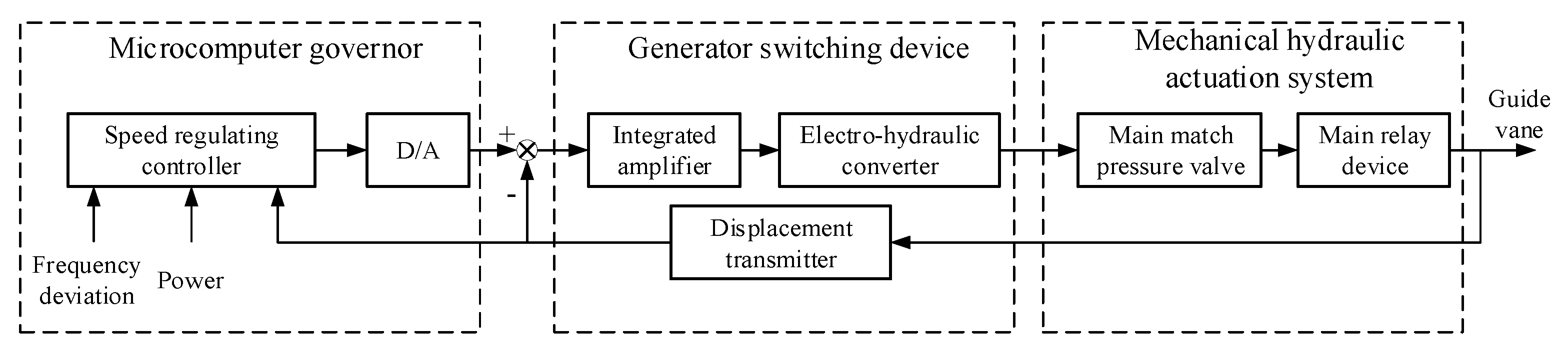
The typical PSU governor consists of a crisis governor and an electro-hydraulic servo system. The basic structure of the governor is shown in Figure 6. The microcomputer regulator is the core of the speed control system. According to the collected information about the speed of the unit, power grid frequency, guide vane opening, and other relevant information, the control mode switching and control signal output functions are realized through the control process and program calculation. The electro-hydraulic servo system converts the electrical output signal of the microcomputer regulator to the displacement signal of the servo motor and drives the water guide mechanism to change the guide vane opening, so as change the flow into the unit runner, finally realizing the regulation control of the unit.

2.4.1. Model of Microcomputer Regulator

In this paper, the numerical simulation of the PSU under the condition of the lower water head is studied by using the microcomputer governor model based on FOPID, which could also be represented as $P{I}^{\lambda }{D}^{\mu }$.

With the development of fractional calculus theory, its application in the control system has been developed rapidly. The research shows that the $P{I}^{\lambda }{D}^{\mu }$ controller has good control performance. In this paper, the $P{I}^{\lambda }{D}^{\mu }$ controller is applied. The $P{I}^{\lambda }{D}^{\mu }$ controller proposed based on the fractional-order differential theory has one more fractional integral order λ and differential order μ than the traditional integral order PID controller. Usually, the λ and μ could be any real numbers in the range of [0, 2] [27]. The structure diagram of the $P{I}^{\lambda }{D}^{\mu }$ controller is shown in Figure 7.

The transfer function of the $P{I}^{\lambda }{D}^{\mu }$ controller is shown as Equation (13).

$$C(s)=\frac{u(s)}{e(s)}=K_p+\frac{K_i}{s^{\lambda }}+K_d{s}^{\mu }$$

(13)

From the above equation, it can be easily concluded that, when both λ and μ are equal to 1, the $P{I}^{\lambda }{D}^{\mu }$ controller equals the traditional PID controller. With two more adjustable parameters, the $P{I}^{\lambda }{D}^{\mu }$ controller not only has all the advantages of the PID controller but also has better flexibility and applicability and can obtain a better control effect.

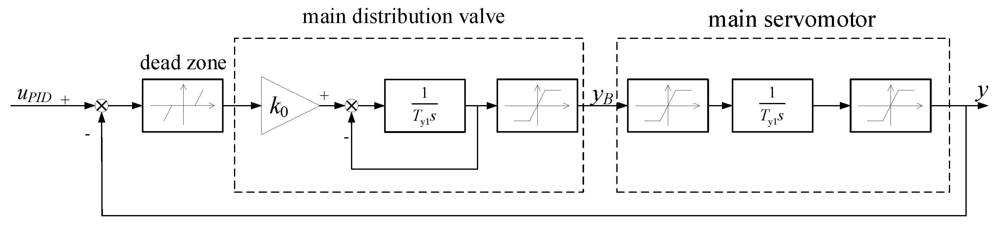
2.4.2. Model of Electro-Hydraulic Servo Motor System

In this paper, the PSUs work in the large fluctuation transition process, and the parameters of the PSU governor change greatly. The nonlinear characteristics of the elector-hydraulic system must be fully taken into account. Therefore, the dead zone, the saturation effect of the main distribution valve, and the main servomotor must be thought about. The structure of the electro-hydraulic servo motor system is shown in Figure 8.

The mathematical expressions are shown as follows:

(1)

the mathematical expression of the dead zone

$$d_{out}=\left\{\begin{array}{l}{d}_{in}-b, d_{in}\ge b\\ 0,\hspace{1em}-a<d_{in}<b\\ d_{in}+b, d_{in}\le -b\end{array}\right.$$

(14)

where b represents the rage of the dead zone; $d_{in}$ represents the input of the dead zone; $d_{out}$ represents the output of the dead zone.

(2)

the mathematical expression of the saturation effect

$$s_{out}=\left\{\begin{array}{l}{s}_{in},\hspace{1em}{s}_{min}<s_{in}<s_{\max }\\ s_{\min },\hspace{1em}{s}_{in}<s_{min}\\ s_{\max },\hspace{1em}{s}_{in}>s_{\max }\end{array}\right.$$

(15)

where s_in represents the input of the saturated nonlinear link; $s_{\max }$ and $s_{\min }$ represents the upper and lower bounds of the saturated nonlinear link, respectively.

In conclusion, in this section, the schematic of the numerical simulation model is shown in Figure 9.

2.5. The Influence of the Interval Time of Successive Start-Up on the Dynamic Characteristics of PSUs

There are hydraulic connections between the two PSUs of the same hydraulic unit in the steady-state operation and transition process. During the process of successive start-up, the hydraulic disturbance in the system will aggravate the change of flow and water pressure in the system, which means a more unfavorable dynamic process. The hydraulic interference will lead to the different transition processes of the two units with different successive start-up interval times.

To figure out the most adverse starting interval time, when the two hydraulic coupling units start up successively under low-water-head conditions. The simulation research about the influence of the interval time ΔT has been carried out based on a model of two hydraulic coupling PSU regulation systems. The physical parameters and working-condition parameters of the model are shown in

Table 2. The physical parameters and working-condition parameters of the model.

Components	Values
Water head	Hu = 716 m Hl = 190 m Hmin = 526 m Hs = 540 m Hmax = 554 m
Suter transformation	k1 = 10 k2 = 0.9 Cy = 0.2 Ch = 0.5
Generator	J = 96.84 tm2
Governor	TID = 1 s T = 0.1 s k0 = 7 TyB = 0.05 Ty = 0.3 s
Direct guide vane control	kc = 1/27

. Under the different water-head operating conditions, with different interval times, the rapidity and stationarity of the units are analyzed during the progress of successive start-ups. The simulation tests are based the MATLAB 9.2. The rapidity is quantitatively characterized by the rise time T_r of the rotating speed, while stationarity is quantitatively characterized by the integral time absolute error (ITAE) of the rotating speed, a relatively comprehensive index. Then the dynamic process of the evaluation index of the unit successive start-up process when the ΔT takes on different values is recorded and compared. The results of the simulation study are as follows.

Figure 10a shows the function between the $\mathrm{\Delta }T$ and T_r of the two PSUs under three different water-head conditions. Under three different water-head conditions, the curves can be divided into three sections according to the status of the fluctuation:$\mathrm{\Delta }T\in \left[0,6\mathrm{s}\right]$,$\mathrm{\Delta }T\in \left(6\mathrm{s},20\mathrm{s}\right]$ and $\mathrm{\Delta }T\in \left(20\mathrm{s},50\mathrm{s}\right]$. Specifically, in the range of $\mathrm{\Delta }T\in \left[0,6\mathrm{s}\right]$, the T_r changes little under three different conditions and the interval time has little effect on it. In the range of $\mathrm{\Delta }T\in \left(6\mathrm{s},20\mathrm{s}\right]$, the T_r curves have a severe fluctuation under all of the three different conditions. Moreover, with the water head decreasing, the fluctuation is more severe. In the range of $\mathrm{\Delta }T\in \left(20\mathrm{s},50\mathrm{s}\right]$, under the conditions of 554 m and 540 m, the T_r is almost a constant with different $\mathrm{\Delta }T$. But under the condition of 526 m, the T_r increase with the increase of $\mathrm{\Delta }T$.

Figure 10b shows the function between the $\mathrm{\Delta }T$ and ITAE of the two PSUs under three different water-head conditions. The ITAE curves are similar under the conditions of 554 m and 540 m. The variation curves of ITAE showed a trend of decreasing firstly, then increasing, and finally decreasing again, and the variation law was relatively simple. However, under the 526 m conditions, the ITAE curve has a more complex fluctuation. Especially in the range of $\mathrm{\Delta }T\in \left[0,8\mathrm{s}\right]$, the ITAE decreases with the increase of $\mathrm{\Delta }T$. Then in the range of $\mathrm{\Delta }T\in \left(8\mathrm{s},20\mathrm{s}\right]$, the curve of ITAE fluctuates irregularly with the increase of $\mathrm{\Delta }T$. In the range of $\mathrm{\Delta }T\in \left(20\mathrm{s},50\mathrm{s}\right]$, the ITAE curve is similar to the other two conditions, and the value of the ITAE increases firstly with the $\mathrm{\Delta }T$ increases, then decreases again.

To sum up, under different conditions with different water-heads, during the progress of the hydraulic coupling PSUs successive start-up, with the increase of $\mathrm{\Delta }T$, the value of T_r and ITAE changes greatly. This is due to the fact that, when the $\mathrm{\Delta }T$ different, the operation state of 1#PSU is completely different than when the 2#PSU is started, and the hydraulic environment and water shock wave in the diversion system must be very different. Therefore, with different $\mathrm{\Delta }T$, the values of T_r and ITAE show great changes. Especially under the conditions of H_min = 526 m, compared to other conditions, with different $\mathrm{\Delta }T$, the influence of the hydraulic disturbance between two PSUs is more complicated on the dynamic progress of successive start-ups.

3. Optimization Schemes

In this section, the multi-objective grey wolf optimizer algorithm (MOGWO) has been used to solve the successive start-up strategy of two hydraulic coupling PSUs under low-water-head extreme conditions. MOGWO, with the characteristics of simple principle, few parameters to adjust, fast convergence, and strong global search ability, has been widely used in solving multi-objective optimization problems.

3.1. Optimization Algorithm

The optimization process of MOGWO is shown as follows.

Step 1: Assigning suitable values to related parameters, including the number of optimization variables; the number of gray waves individuals, n; maximum iterations M, and the number of Pareto archives, and other basic parameters for multi-optimization, such as the grid inflation parameter, the number of grids per each dimension, leader selection pressure parameter, and extra repository member selection pressure.

Step 2: Initializing the variable to be optimized X_i(k) (i = 1, 2, … n), and k represents the number of iterations.

Step 3: Inputting X to the model of successive start-up, calculating the fitness function and position vectors of every individual, and judge whether the constraint conditions are satisfied. If the answer is yes, then it is ready for the next step; if not, then it is best to return to Step 1.

Step 4: Comparing the fitness function of each individual, determining the dominant relationship between individuals, saving the non-dominated individuals in the Pareto archive.

Step 5: Calculating the distance for each Pareto archive individual and choosing the α, β, and δ gray waves individuals; the α, β, and δ represent the best, second-best, and third-best solutions respectively, and they are the leaders of the herd that in the Pareto archive and others are named as w.

Step 6: Updating the position of the current w individuals with Equations (16)–(18)

$$\left\{\begin{array}{l}{D}_{\alpha }=\left|C_1\cdot X_{\alpha }-X_{\left(k\right)}\right|\\ D_{\beta }=\left|C_2\cdot X_{\beta }-X_{\left(k\right)}\right|\\ D_{\delta }=\left|C_3\cdot X_{\delta }-X_{\left(k\right)}\right|\end{array}\right.$$

(16)

$$\left\{\begin{array}{l}{X}_1=X_{\alpha }-A_1\cdot D_{\alpha }\\ X_2=X_{\beta }-A_2\cdot D_{\beta }\\ X_3=X_{\delta }-A_3\cdot D_{\delta }\end{array}\right.$$

(17)

$$X_{\left(k+1\right)}=\frac{X_1+X_2+X_3}{3}$$

(18)

where both the A and C are coefficient vectors.

Step 7: Calculating the value of fitness, comparing it with the individuals in the Pareto archive of the $\left(k-1\right)th$ generation, and updating the Pareto archive according to the dominance relationship.

Step 8: Calculating the distance between each individual in the Pareto archive, and, if the number of non-dominated individuals is more than the archive size, removing some individuals, as many as necessary according to the archive size.

Step 9: Updating the best, second-, and third-best solution.

Step10: Determining whether the maximum iteration criteria are satisfied; if the answer is yes, it is best to return to Step 6, and if not, output the optimal Pareto solution is the next step.

The optimization process is shown in Figure 11.

3.2. Objective Function

Researchers pay more attention to the rapidity and stationarity of a unit when it starts up. Rapidity is quantitatively characterized by the rise time of the rotating speed, while stationarity is quantitatively characterized by the integral time absolute error (ITAE) of the rotating speed, a relatively comprehensive index. However, the rapidity and stability are irreconcilable, so it is impossible to get the best result for the two indices at the same time. In actual production, usually the aim is to achieve the optimal combination of these two performance indices. In this study, select the sum of the rise time of the rotating speed of two PSUs and the sum of the ITAE of two PSUs as the objective function. The two optimization objectives can be expressed as Equation (19).

$$\left\{\begin{array}{l}\min f_1=T_{r1}+T_{r2}\\ \min f_2=ITA{E}_1+ITA{E}_2\end{array}\right.$$

(19)

3.3. Optimizer Variables

During the process of start-up, the guide vane opening change process is shown in Figure 12. In the figure, θ represents the inclination angle of the guide vane opening ascending process line, and k_c represents the maximum velocity of guide vane opening change. The $y_c$ represents the maximum relative opening of the guide vane during the start-up process. In this study, the k_c has been set as 1/27.

$y_c$ and the controller parameters are selected as the optimization variables. In Section 2, interval time had great influence on the process of successive start-up and should be selected as an optimization variable. Moreover, due to the different operation statuses during successive start-ups, the two hydraulic coupling PSUs should own different control parameters, and the optimization variables in the two cases are shown as Equations (20) and (21), respectively.

$$X_1=(K_p,K_i,K_d,y_c,\mathrm{\Delta }T)$$

(20)

$$X_2=(K_{p1},K_{i1},K_{d1},{\lambda }_1,{\mu }_1,y_c{}_1,\mathrm{\Delta }T,K_{p2},K_{i2},K_{d2},{\lambda }_2,{\mu }_2,y_c{}_2)$$

(21)

On the right side of Equation (20), subscript 1 and 2 represent the 1# PSU and 2# PSU, respectively.

3.4. Constraint Conditions

In the actual production process, there are specific constraints on the relevant indicators of the start-up process. In this paper, three constraints are mentioned as follows.

(1)

The upper and low boundaries of the optimization variables X

$$X\in \left[L,U\right]$$

(22)

where L and U represent the upper and lower boundaries, respectively. Specific values of the L and U are shown in

Table 3. The boundaries of the optimization variables.

Variables	Boundaries	Values
X1	L1	0.1	0.1	0.1	0.1	1	0.2	0
	U1	10	8	8	1	2	0.3	40
X2	L2	0.1	0.1	0.1	0.1	1	0.2	0	0.1	0.1	0.1	0.1	1.0	0.2
	U2	10	8	8	1	2	0.3	40	10	8	8	1	2.0	0.3

.

(2)

Oscillation times of rotation speed

According to the requirements of the start-up transition process of the PSUs, the number of rotation speed oscillations shall not exceed two times.

(3)

Limitation of water hammer pressure

The water hammer pressure of each link in the system shall not exceed the upper limit obtained by regulation guarantee calculation.

4. Numerical Calculation Experiment of Successive Start-Up under Low-Water-Head Extreme Conditions

In the real station, there are two main guide vane opening strategies for PSUs, one-stage starting and two-stage starting. The control methods used by these two methods are traditional PID control. However, under low-water-head extreme working conditions, the pumped storage unit can easily fall into the ‘S’ region during the process of start-up, and it’s difficult for the PID controller to obtain an excellent control effect. The fractional-order PID (FOPID) has two more adjustable parameters than the traditional PID, so it has better control flexibility and can obtain a better adjustment effect. In this paper, two schemes are compared with others. Specifically, the controller and the parameters in the study on the successive start-up process are variable. PIDDP and FOPIDDP are researched respectively in this paper.

A pumped storage station in China has been selected as the reference system for this study, and the relevant parameters are the same as this real station. An accurate model of the speed regular system of two hydraulic coupling PSUs has been proposed, and a simulation study has performed in MATLAB 9.2. Two kinds of strategies for successive start-up under low conditions have been researched in this paper.

In this paper, set the number of gray wave individuals $n=100$, and the maximum iterations $M=300$. The results of the optimization of successive start-up strategies with two different controllers are as follows.

In this paper, the optimization result is a Pareto archive, which consists of a series of non-inferior solutions. Figure 13 shows the Pareto archive, and the value of the optimization variables in the Pareto archive are listed in Appendix A 

Table A1. Pareto archive under PID controller.

Solutions	${\mathit{K}}_{\mathit{p}1}$	${\mathit{K}}_{\mathit{i}1}$	${\mathit{K}}_{\mathit{d}1}$	${\mathit{y}}_{\mathit{c}1}$	${\mathit{K}}_{\mathit{p}2}$	${\mathit{K}}_{\mathit{i}2}$	${\mathit{K}}_{\mathit{d}2}$	${\mathit{y}}_{\mathit{c}2}$	$\mathbf{\Delta }\mathit{T}$
1	1.1925	4.7705	3.8386	0.3000	1.0264	3.7686	1.7617	0.3000	24.8353
2	1.1841	4.8417	3.8247	0.3000	1.0211	3.7870	1.8279	0.3000	25.7208
3	0.8434	4.8025	3.3461	0.2991	0.5425	3.5893	1.7219	0.2956	15.2920
4	0.8220	4.7674	3.5252	0.2996	0.5409	3.6460	1.7732	0.2903	15.4059
5	0.8548	4.8194	3.3967	0.3000	0.5542	3.6370	1.8115	0.3000	15.4788
6	0.8144	4.6661	3.6072	0.3000	0.5509	3.5573	1.8191	0.2971	15.4504
7	0.8385	4.7589	3.3806	0.2990	0.5413	3.5597	1.7238	0.2946	15.4116
8	0.8146	4.7299	3.6102	0.3000	0.5489	3.6101	1.7905	0.2919	15.4256
9	0.8197	4.6696	3.6107	0.2998	0.5541	3.5570	1.8281	0.2969	15.5383
10	0.8203	4.6707	3.6111	0.3000	0.5522	3.5608	1.8247	0.2976	15.5976
11	0.8715	4.7503	3.6393	0.2999	0.5895	3.6629	1.7932	0.2901	15.5248
12	0.6285	4.7633	3.9859	0.2996	0.6314	3.9650	1.6867	0.2998	27.8300
13	0.8225	4.6906	3.6173	0.3000	0.5542	3.5862	1.8210	0.2959	15.7242
14	0.6425	4.7612	3.9762	0.2999	0.6399	3.9593	1.6977	0.2998	27.6187
15	1.0271	4.6495	3.5825	0.3000	0.6910	3.6774	1.7781	0.3000	15.4626
16	0.8545	4.8164	3.4118	0.3000	0.5541	3.6412	1.8111	0.2997	15.6067
17	1.2055	4.8233	3.8714	0.3000	0.9807	3.8226	1.9135	0.3000	25.5276
18	0.7513	4.8524	3.9405	0.3000	0.6625	3.9626	1.8100	0.3000	27.1635
19	0.5686	4.7506	3.9798	0.2984	0.6008	3.9461	1.6692	0.2993	27.8832
20	0.6550	4.7633	3.9743	0.2999	0.6573	3.9548	1.6987	0.2999	27.6223
21	0.8556	4.7457	3.6342	0.2996	0.5829	3.6513	1.7865	0.2899	15.2710
22	0.8477	4.7970	3.4457	0.3000	0.5569	3.6209	1.7398	0.2968	15.7298
23	0.8606	4.7962	3.3957	0.2999	0.5633	3.6284	1.8035	0.2999	15.4701
24	1.1936	4.7938	3.8537	0.3000	1.0299	3.7861	1.8083	0.3000	25.0752
25	0.6059	4.7542	3.9805	0.2986	0.6285	3.9491	1.6773	0.2994	27.8763
26	1.0301	4.9349	3.8476	0.3000	0.7399	3.9261	1.8736	0.3000	25.9410
27	1.1878	4.8585	3.8922	0.3000	0.9429	3.8568	1.9236	0.3000	25.6958
28	1.1430	4.9518	3.9508	0.3000	0.8703	3.9426	2.2738	0.3000	24.9287

and

Table A2. Pareto archive under FOPID controller.

Solutions	${\mathit{K}}_{\mathit{p}1}$	${\mathit{K}}_{\mathit{i}1}$	${\mathit{K}}_{\mathit{d}1}$	${\mathit{\lambda }}_1$	${\mathit{\mu }}_1$	${\mathit{y}}_{\mathit{c}1}$	${\mathit{K}}_{\mathit{p}2}$	${\mathit{K}}_{\mathit{i}2}$	${\mathit{K}}_{\mathit{d}2}$	${\mathit{\lambda }}_2$	${\mathit{\mu }}_2$	${\mathit{y}}_{\mathit{c}2}$	$\mathbf{\Delta }\mathit{T}$
1	1.179	1.673	5.567	0.296	1.077	0.298	1.262	1.997	5.421	0.146	1.053	0.296	28.58
2	1.178	1.673	5.563	0.296	1.076	0.298	1.262	1.988	5.420	0.146	1.053	0.296	28.57
3	1.136	1.680	5.504	0.292	1.077	0.298	1.268	1.985	5.470	0.146	1.065	0.299	28.58
4	1.173	1.687	5.524	0.297	1.082	0.297	1.293	2.000	5.480	0.144	1.062	0.300	28.52
5	1.070	1.662	5.459	0.298	1.072	0.297	1.281	1.955	5.343	0.149	1.054	0.295	28.53
6	1.075	1.665	5.472	0.297	1.072	0.297	1.277	1.964	5.351	0.148	1.055	0.296	28.57
7	1.075	1.666	5.472	0.297	1.072	0.297	1.278	1.964	5.355	0.148	1.056	0.296	28.58
8	1.139	1.700	5.423	0.300	1.059	0.298	1.270	2.000	5.500	0.150	1.061	0.300	28.25
9	1.138	1.694	5.453	0.300	1.066	0.298	1.274	2.000	5.486	0.149	1.067	0.299	28.47
10	1.133	1.692	5.472	0.300	1.067	0.298	1.272	1.998	5.476	0.149	1.066	0.299	28.45
11	1.137	1.694	5.452	0.300	1.066	0.298	1.273	1.999	5.484	0.149	1.066	0.299	28.45
12	1.139	1.694	5.460	0.300	1.067	0.298	1.274	2.000	5.486	0.149	1.068	0.299	28.50
13	1.139	1.700	5.425	0.300	1.059	0.298	1.270	2.000	5.500	0.150	1.061	0.300	28.26
14	1.143	1.674	5.574	0.296	1.076	0.298	1.277	1.989	5.435	0.148	1.074	0.299	28.56
15	1.130	1.670	5.545	0.296	1.076	0.298	1.273	1.983	5.434	0.148	1.071	0.297	28.58
16	1.107	1.678	5.492	0.292	1.077	0.298	1.263	1.967	5.396	0.147	1.060	0.292	28.58
17	1.134	1.670	5.551	0.296	1.076	0.298	1.275	1.983	5.428	0.148	1.071	0.297	28.56
18	1.132	1.672	5.549	0.295	1.076	0.298	1.274	1.982	5.422	0.148	1.071	0.297	28.55
19	1.141	1.676	5.569	0.296	1.076	0.298	1.275	1.986	5.436	0.148	1.074	0.299	28.58
20	1.141	1.673	5.569	0.296	1.076	0.298	1.277	1.987	5.433	0.148	1.073	0.299	28.56
21	1.056	1.651	5.476	0.290	1.067	0.299	1.277	1.972	5.335	0.150	1.080	0.300	28.35
22	1.156	1.686	5.581	0.296	1.077	0.299	1.280	1.994	5.446	0.149	1.075	0.300	28.52
23	1.152	1.683	5.575	0.296	1.076	0.298	1.279	1.990	5.444	0.149	1.074	0.300	28.50
24	1.058	1.654	5.477	0.290	1.067	0.299	1.279	1.973	5.342	0.150	1.080	0.300	28.37
25	1.129	1.671	5.537	0.295	1.076	0.298	1.272	1.982	5.425	0.149	1.069	0.297	28.60
26	1.143	1.674	5.574	0.296	1.076	0.298	1.277	1.989	5.435	0.148	1.074	0.299	28.56
27	1.130	1.670	5.545	0.296	1.076	0.298	1.273	1.983	5.434	0.148	1.071	0.297	28.58
28	1.141	1.677	5.566	0.295	1.076	0.299	1.275	1.986	5.437	0.148	1.073	0.299	28.56
29	1.110	1.678	5.497	0.292	1.077	0.298	1.263	1.966	5.393	0.147	1.062	0.292	28.59
30	1.107	1.678	5.492	0.292	1.077	0.298	1.263	1.967	5.396	0.147	1.060	0.292	28.58
31	1.134	1.670	5.551	0.296	1.076	0.298	1.275	1.983	5.428	0.148	1.071	0.297	28.56
32	1.132	1.672	5.549	0.295	1.076	0.298	1.274	1.982	5.422	0.148	1.071	0.297	28.55
33	1.141	1.676	5.569	0.296	1.076	0.298	1.275	1.986	5.436	0.148	1.074	0.299	28.58

. As shown in Figure 13, the Pareto archive under PID control is dominated by the Pareto archive under FOPID control. In other words, it is indicated that the FOPID controller obtains a better Pareto archive than the traditional PID controller.

In this paper, we use the method of relative objective proximity [28] to obtain the best solution under the two different controllers as shown in Figure 13. The value of these two solutions is shown in

Table 4. Optimal solution of the best solution.

Schemes	Kp1	Ki1	Kd1	λ1	μ1	yc1	ΔT	Kp2	Ki2	Kd2	λ2	μ2	yc2
PIDDP	0.8220	4.7674	3.5252			0.2996	15.4059	0.5409	3.6460	1.7732			0.2903
FOPIDDP	1.137	1.694	5.452	0.300	1.066	0.298	28.45	1.273	1.999	5.484	0.149	1.066	0.299

.

Inputting the best solution to the control system of the PSUs, we can obtain the dynamic processes of the performance indexes, including the rotating speed, flow, and actual working water-head curves during the process of successive start-up under low extreme water-head conditions, shown in Figure 14, Figure 15 and Figure 16. The start-up process curves of the two PSUs, respectively, during the successive start-up process of the two schemes in the full-characteristic curves are shown in Figure 17 and Figure 18.

The maximum and the rise time of the rotational speed were recorded, and the oscillation number of the rotational speed of the four schemes is shown in

Table 5. The quantitative index of the rotational speed.

Schemes	1#PSU		2#PSU
	Maximum (p.u.)	Rise Time (s)	Number of Oscillation	Maximum (p.u.)	Rise Time (s)	Number of Oscillation
PIDDP	1.02	20.74	2	1.017	20.64	1
FOPIDDP	1.009	20.66	1	1.019	19.99	0

.

Figure 14 shows the dynamic process of the rotational speed of the two PSUs, respectively, during the successive start-up process under low- water-head extreme conditions with two different controllers. It is easy to get that the rotational speed rise time is approximate for the two coupling PSUs under two different controllers; to be specific, the difference value is within 1 s. For the 1# PSU alone, the speed rise time has little difference under two different controllers. However, the overshoot of the rotational speed is smaller under the FOPID controller than under the PID. The dynamic process of the FOPID controller is much better with smaller oscillation, stability time, and steady-state error. For the 2# PSU alone, we can obtain that the rotational speed overshoot under the two controllers is greatly approximate. However, the dynamic curves of the rotational speed are more approximate under the FOPID, with the smallest number of oscillations. In conclusion, combined with Figure 14 and Table 5, it is obvious that the rotational speed indicators under the FOPID are better than under the traditional PID.

Figure 15 shows the dynamic process of the flow of the two PSUs, respectively, during the successive start-up process under low-water-head extreme conditions with two different controllers. In Figure 15a, for the 1# PSU alone, before the unit flow curve come to the first wave peak, the control of the PSUs is in the open-loop stage, so the flow dynamic process is roughly the same with two different controllers. When the simulation time $t=\mathrm{\Delta }T$, with the 2# PSU start-up, due to the water interference in the diversion system, the flow curves of unit 1# all have obvious oscillations. After that, closed-loop adjustment is carried out under PID and FOPID control strategies, respectively. As shown in Figure 15a, the flow dynamic process curves of 1# PSU have an obvious under different controllers when $t\in \left[20s,50s\right]$. Moreover, under the FOPID, the flow oscillation attenuation is faster. As shown in Figure 15b, the flow dynamic process of unit 2# is similar under two different controllers, and both can quickly decay to the steady-state.

Figure 16 shows the dynamic process of the actual working water head of the two PSUs, respectively, during the successive start-up process under low-water head extreme conditions with two different controllers. The value of the water head is relative to the H_s. Compared to the dynamic curves of the two PSUs, it is obvious that the start-up of 2# PSU could lead to a considerable oscillation in the process of the 1# PSU. At the same time, the hydraulic interference between the two PSUs will also cause a violent oscillation of the dynamic process curve of 2# PSU. Combining the actual working water-head dynamic curves of the two PSUs with different controllers, the dynamic process of the two PSUs are roughly similar in general, but the oscillation attenuation of the dynamic process curve under the FOPID is faster.

Figure 17 and Figure 18 shows the start-up process curves in the full-characteristic curves of the two PSUs, respectively, during the successive start-up process under low-water-head conditions. For 1# PSU, as shown in Figure 17, the start-up process curves can avoid falling into the reverse ‘S’ region better under the FOPID. However, under the traditional PID, the start-up process curves fall into the reverse ‘S’ region, and both the flow characteristics and torque characteristics show reciprocating oscillations in this region. For 2# PSU, as shown in Figure 18, the start-up process curves can better avoid falling into the reverse ‘S’ region under the FOPID. However, under the traditional PID, only the flow characteristics can avoid falling into the reverse ‘S’ region, but torque characteristics also show reciprocating oscillations in this region. It can be summed up that, with the FOPID, the two PSUs can avoid falling into the reverse ‘S’ region better during the process of successive start-up under low-water-head extreme conditions.

5. Conclusions

The successive start-up strategy of two hydraulic coupling PSUs under low-water-head extreme conditions was studied in this paper. An accurate model of successive start-up was established. The influence of interval time on the dynamic characteristics of successive start-up was analyzed. A novel optimization scheme with FOPIDDP was proposed for successive start-up. For comparison, the optimization scheme PIDDP was also tested. Moreover, MOGWO was adopted to solve the Pareto archive of the parameters of novel optimization schemes. All numerical simulation experiments were completed in MATLAB 9.2.

Several conclusions can be extracted from this study:

(1)

The interval time ΔT could make a great influence on the successive start-up process; when ΔT is greater than a certain value, the instability of the PSUs will be intensified, especially for 1# PSU. Operating teams can refer to the research results of this paper to select the optimal interval time.

(2)

The results show that the multi-objective optimization aiming at the speed rise time and ITAE value of the two units can effectively reduce the risk of falling into the anti-S instability zone when the units are successively started at low-water-head conditions.

(3)

With muti-objective optimization, the Pareto archive provides a series of feasible solutions for decision-makers. Based on the result, the operating teams can select the optimal solution according to their actual demand and therefore can obtain the maximum benefit.

(4)

The multi-objective optimization method with FOPID is feasible and conducive to avoiding the ‘S’ region during the process of successive start-up under-low-water head extreme conditions.

The results of this paper are helpful in solving the difficulty of regulating and controlling the hydraulic coupling PSUs under low-head conditions.