Article

Modeling of an Elastocaloric Cooling System for Determining Efficiency

1
Fraunhofer Institute for Physical Measurement Techniques IPM, Georges-Koehler-Allee 301, 79110 Freiburg, Germany
2
Institute of Internal Combustion Engines IFKM, Karlsruhe Institute of Technology (KIT), 76131 Karlsruhe, Germany
*
Author to whom correspondence should be addressed.
Energies 2022, 15(14), 5089; https://doi.org/10.3390/en15145089
Submission received: 22 June 2022 / Revised: 8 July 2022 / Accepted: 8 July 2022 / Published: 12 July 2022
(This article belongs to the Special Issue Advanced Thermal Management and Cooling Technologies)

Abstract

:
When it comes to covering the growing demand for cooling power worldwide, elastocalorics offer an environmentally friendly alternative to compressor-based cooling technology. The absence of harmful and flammable coolants makes elastocalorics suitable for energy applications such as battery cooling. Initial prototypes of elastocaloric systems, which transport heat by means of thermal conduction or convection, have already been developed. A particularly promising solution is the active elastocaloric heat pipe (AEH), which works with latent heat transfer by the evaporation and condensation of a fluid. This enables a fast and efficient heat transfer in a compression-based elastocaloric cooling system. In this publication, we present a simulation model of the AEH based on MATLAB-Simulink. The model showed very good agreement with the experimental data pertaining to the maximum temperature span and maximum cooling power. Hereby, non-measurable variables such as efficiency and heat fluxes in the cooling system are accessible, which allows the analysis of individual losses including the dissipation effects of the material, non-ideal isolation, losses in heat transfer from the elastocaloric material to the fluid, and other parasitic heat flux losses. In total, it can be shown that using this AEH-approach, an optimized system can achieve up to 67% of the material efficiency.

1. Introduction

Global demand for cooling power is growing [1] and is currently met almost exclusively by compressor-based cooling technology. This technology, however, often involves harmful refrigerants. Elastocaloric cooling systems offer an efficient, environmentally friendly alternative that is free from harmful refrigerants [2]. These cooling systems use elastocaloric materials (ECM) such as nickel-titanium alloys [3]. When mechanical tensile, compressive, or bending loads are applied to ECMs, their structure changes from the austenitic to the martensitic phase, releasing latent heat. If this heat is dissipated and the load subsequently removed from the ECM, it will cool down below its initial temperature. This reversible process is known as the “elastocaloric effect” [3]. Cyclically repeating this effect enables heat to be pumped from a cold to a warm reservoir and thus create a cooling system.
Essential for the performance of such an elastocaloric cooling system is the heat transfer between an elastocaloric material and heat source and sink. There are various ways of transferring this heat: in thermal conduction systems, the ECM alternately contacts the system’s heat source and the heat sink [4,5,6,7,8]. In these systems, materials are used as thin films or wires with a large surface area for heat exchange under tensile stress. Heat can also be transported by a fluid or gas using forced convection [9,10,11,12,13,14,15,16,17]. These systems are often set up as regenerators to increase the temperature range. In recent years, several system approaches with compressive stress have been presented to improve the long-term stability of these systems. Another approach used bending stress and combined both heat transfer mechanisms (conduction and convection) [18]. A third way is to use latent heat transfer, which is a very efficient and fast method of transferring heat and has been used in heat pipes for decades. The active elastocaloric heat pipe (AEH) approach, which utilizes this heat transfer method, has already been shown to be able to generate a temperature span of 5.6 K and a specific cooling power of 6.3 W/g, while showing very good long-term stability under compressive loading [19].
Simulations are an important tool for improving such elastocaloric cooling systems. Validated with experimental data, they can be used to quantify variables that are not directly measurable such as individual loss factors such as parasitic heat fluxes, pressure loss in the valves, and heat exchanger losses. Furthermore, the system’s efficiency can be quantified and compared to the theoretical limit given by the properties of the elastocaloric material, enabling the quantification of further optimization potential. In the literature, different approaches of elastocaloric cooling systems have been studied regarding their efficiency with simulations [20,21,22,23]. In this publication, we present a simulation model of the AEH that was validated with experimental data. Our aims were to determine potential improvements and draw conclusions on the system efficiency that could be achieved.
To model the materials’ behavior, a thermodynamically consistent model based on an approximation of the heat capacity curve by a Cauchy–Lorentz distribution was used. The adiabatic temperature change and dissipative energy of the material can be analytically derived from this equation and expressed as a function of mechanical stress and temperature [24]. Non-measurable input variables such as thermal resistance in the cooling system were determined in advance using an analytical model as described below.

2. Materials and Methods

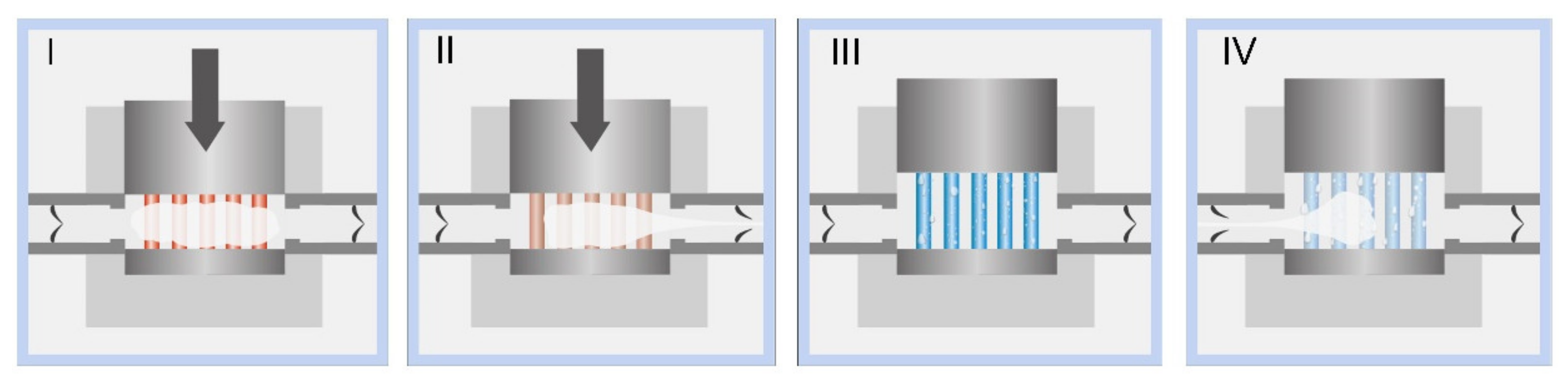
2.1. Active Elastocaloric Heat Pipe

In the AEH concept, the heat is transferred between the elastocaloric material, heat sink, and source by evaporation and condensation. This method of heat transfer has been used in standard heat pipes for many decades. A heat pipe is a hermetically sealed container where only the fluid is present in its liquid and gaseous states and all non-condensable gases have been removed. In such a heat pipe, a small increase in temperature on one side of the heat pipe (evaporator) directly leads to evaporation of the liquid fluid, an increase in the vapor pressure, and the condensation of the gaseous fluid on the other side of the heat pipe (condenser). Due to the very large latent heat of the evaporation and condensation process, a lot of thermal energy can be transferred with very small amounts of fluid, resulting in very good thermal transport properties of heat pipes.
In the AEH, the same concept is used for heat transfer. The AEH consists of an evaporator (cold side), a segment with the ECM and a condenser (warm side). The segment is separated from the condenser and the evaporator by passive check valves to direct the flow of the gaseous fluid and thereby the heat flux. The working principle of the AEH is shown schematically in four consecutive time steps in Figure 1: (I) When a load is applied to the ECM, it warms up and the fluid on the surface evaporates, so the pressure in the segment increases; (II) the check valve on the condenser side opens and the gaseous fluid streams into the condenser; and (III) when the load is removed from the ECM, it cools down. The fluid condenses on the ECM, the pressure in the segment decreases and gaseous fluid streams from the evaporator into the segment through the check valve (IV).
Such an AEH with one segment has been built and characterized, the details are described in [19]. As the ECM, nine tubular samples of commercially available Ni56.16Ti43.84 with an outer diameter of 2.4 mm and a wall thickness of 0.3 mm and a total mass 1.32 g were used. These tubes were loaded with a compressive stress of 836 MPa by an external press. The evaporator is a copper tube that is insulated from the environment with polyethylene foam. A heating wire is wrapped around the evaporator in order to apply a defined thermal load. The condenser is attached to an external chiller unit to keep it at a constant temperature. The condensed fluid in the condenser can be led back to the evaporator through a throttle. Water was used as the fluid.

2.2. System Simulation

To calculate the efficiency and identify potential improvements of the AEH, we implemented a simulation of the AEH in MATLAB Simscape. The simulation takes into account the time-related as well as the nonlinear material behavior. Figure 2 shows a conceptual sketch of the simulation setup. The fluid loop is shown in blue using elements of the two-phase fluid model, which takes into account the fluid properties of the gaseous or liquid state. Thermal data such as heat flows were calculated using the Simscape thermal model and are shown in red. The simulation consists of three components: the evaporator (bottom), the segment with the ECM (middle), and the condenser (top). These were implemented in the simulation using the saturated fluid chamber block from the Rankine cycle MATLAB example. In this block, thermal and fluid data are combined, resulting in a transition between the liquid and gaseous states of the fluid. The material behavior was implemented using the material model previously published in [24] with the following ECM parameters: T 0 = 273.9 K, temperature at maximum heat capacity with no applied field; Δ s iso , max = 42.7 J/(kg K), maximum isothermal entropy change; c 0 = 663.6 J/(kg K), heat capacity far from the transformation peak; α = 26.8 K, width of the heat capacity peak; and β = 0.0845 K/MPa, the multiplicative inverse of the Clausius–Clapeyron coefficient [24].
As in the experiments, these three components (evaporator, segment with the ECM, and condenser) were connected by passive check valves in the simulation, which were implemented using a variable local restriction. The pressure data on either side of the valve determine when the valves open in the simulation. The cross section and the proportionality constant are input parameters of the simulation and were determined by fitting the volume flow in the simulation to experimental data. In these experiments, the volume flow of gaseous fluid through these check valves was measured depending on the pressure difference [25]. In Figure 3, the volume flow rates were plotted as a function of pressure. The simulation of the valve showed good agreement with the measured data.
The liquid fluid flows from the condenser to the evaporator through a throttle, which was implemented as a variable local restriction in the simulation. A heat flux flows from the ambience with the temperature T A into the evaporator via the thermal resistance R Iso . The heat flux of the heating wire into the evaporator for the measurements of the cooling power is Q ˙ in . A sinusoidal stress curve is applied to the ECM, which transfers heat to the fluid via the resistance R th . At the same time, the temperature of the ECM is affected by the resistance to the ambient temperature R K since heat is also exchanged with the environment via the contact of the ECM to the outer containment. The condenser was set at ambient temperature in the simulation to reflect the temperature-controlled conditions in the experimental setup.

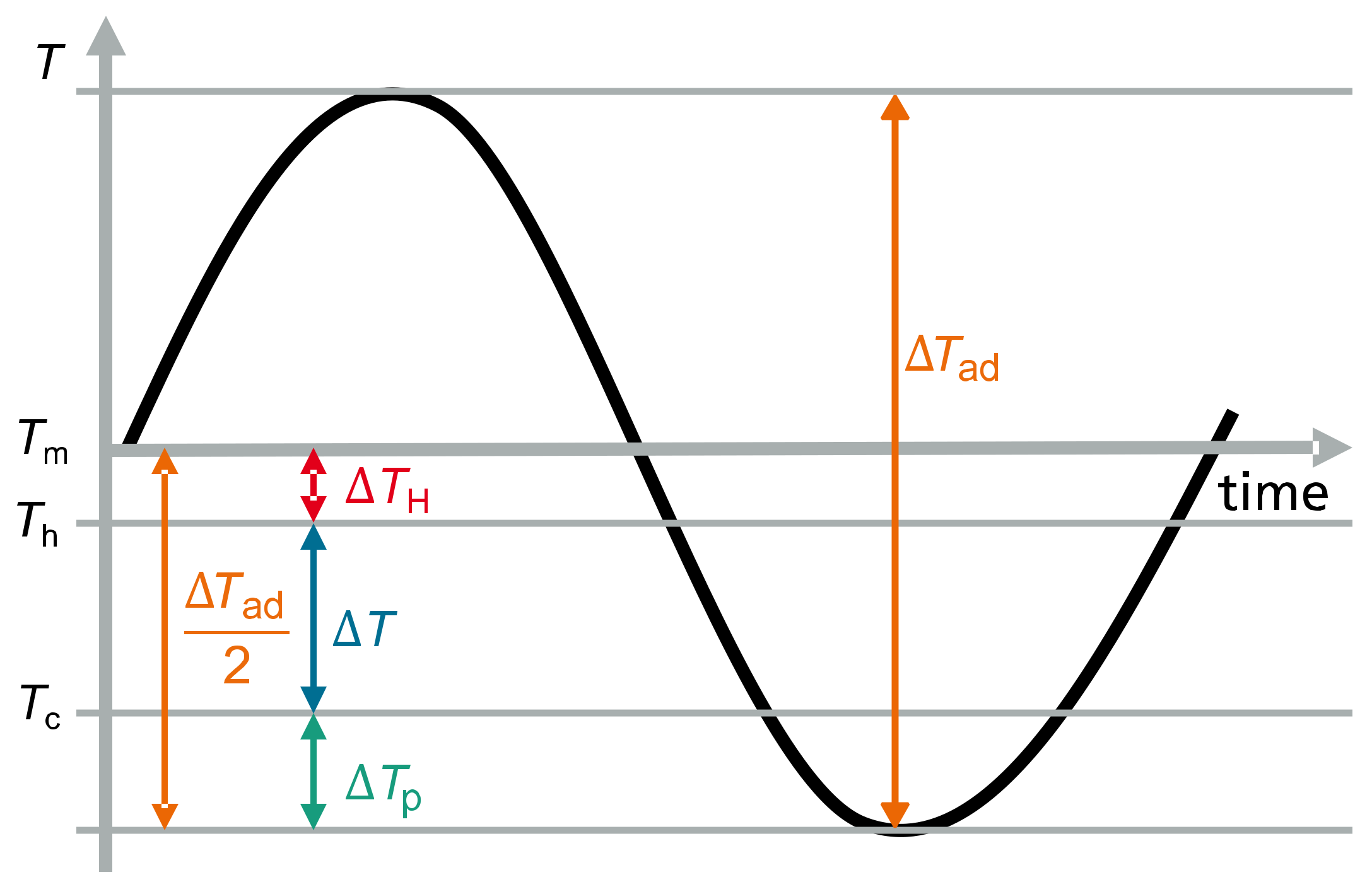
2.3. Analytical Determination of System Parameters

To carry out the simulations, the essential thermal resistances R Iso , R K , and R th must be known. In order to attain a rough estimate of these thermal resistances, we set up a simplified, stationary analytical model (Figure 4). The temperature of the ECM is shown in black. The amplitude is Δ T ad / 2 . The temperature span between the condenser T h and the evaporator T c is Δ T and the temperature change available for pumping heat from the evaporator to the segment is Δ T p .
In the AEH, the ECM absorbs heat from the evaporator and transfers it to the condenser. Dissipation effects cause the ECM to heat up further, and this heat is passed into the environment via the resistance R K . As a result, the mean temperature of the ECM T m is higher than the temperature of the condenser T h . This means that no more than half of the adiabatic temperature change ( Δ T ad / 2 ) can be used to pump heat. In addition, as a result of the dissipative heat q diss , which only flows into the environment via the resistance R K , the usable temperature span decreases by the temperature change Δ T H . This equates to the temperature change between the average material temperature T m and the condenser temperature T h , as shown in Equation (1).
Δ T H = T m T h = q diss m ECM R K f
In this equation, m ECM is the mass of the ECM; f is the system frequency; and q diss is the specific dissipative energy per cycle.
To calculate the cooling power that can be pumped using the AEH, the first step is to calculate the temperature span Δ T p available for this purpose. Δ T p can be calculated as a function of the other temperature changes using Equation (2).
Δ T p = Δ T ad 2 Δ T Δ T H = Δ T ad 2 Δ T q diss m ECM f R K
Pumping performance Q ˙ p = Q ˙ p , max f / 1 + f / f c 2 f c can generally be estimated in relation to the maximum pumping performance Q ˙ p , max f = Δ T ad / 2 π R th and the cut-off frequency f c = 1 / 2 π R th c eff m ECM using Equation (3) [26]. Here, c eff is the actual specific heat capacity. The cut-off frequency f c is the frequency up to which point the maximum cooling power increases in proportion to the frequency. In the model, R th also encompasses thermal resistances resulting from the flow resistance of the gaseous fluid, though this is small compared to the evaporation and condensation resistance and the thermal conduction resistance in the ECM. The effective specific heat capacity c eff can be calculated using the specific isothermal entropy change Δ s iso ; the temperature T and the adiabatic temperature change of the ECM Δ T ad : c eff = Δ s iso T / Δ T ad = 834   J kg K . However, only Δ T p and not Δ T ad is available in the AEH for pumping heat. The heat flux Q ˙ p can therefore be calculated as shown in Equation (3).
Q ˙ p = Q ˙ p , max 1 + f f c 2 f f c = Δ T p c eff m ECM f 1 + f c eff m ECM 2 π R th 2 = c eff m ECM f Δ T ad 2 Δ T q diss m ECM f R K 1 + f c eff m ECM 2 π R th 2
To identify the temperature change Δ T , we assumed that there is a heat flux balance in the evaporator. The output of the heating wire Q ˙ in and the heat flux through the thermal insulation Q ˙ R Iso flow into the evaporator, while Q ˙ p flows into the segment through the valve.
Q ˙ p + Q ˙ in + Q ˙ R Iso = 0 c eff m ECM f Δ T ad 2 Δ T q diss m ECM f R K 1 + f c eff m ECM 2 π R th 2 + Q ˙ in + Δ T R Iso = 0
Solving Equation (4) results in a temperature span of:
Δ T = R Iso c eff m ECM f Δ T ad 2 q diss m ECM f R K R Iso Q ˙ in 1 + f c eff m ECM 2 π R th 2 c eff m ECM f R Iso + 1 + f c eff m ECM 2 π R th 2
The maximum temperature change without applying cooling power is shown in Equation (6).
Δ T Q ˙ in = 0 = R Iso c eff m ECM f Δ T ad 2 q diss m ECM f R K c eff m ECM f R Iso + 1 + f c eff m ECM 2 π R th 2
The maximum cooling power of the system can be calculated using Equation (7).
Q ˙ max Δ T = 0 = c eff m ECM f Δ T ad 2 q diss m ECM f R K 1 + f c eff m ECM 2 π R th 2

3. Results

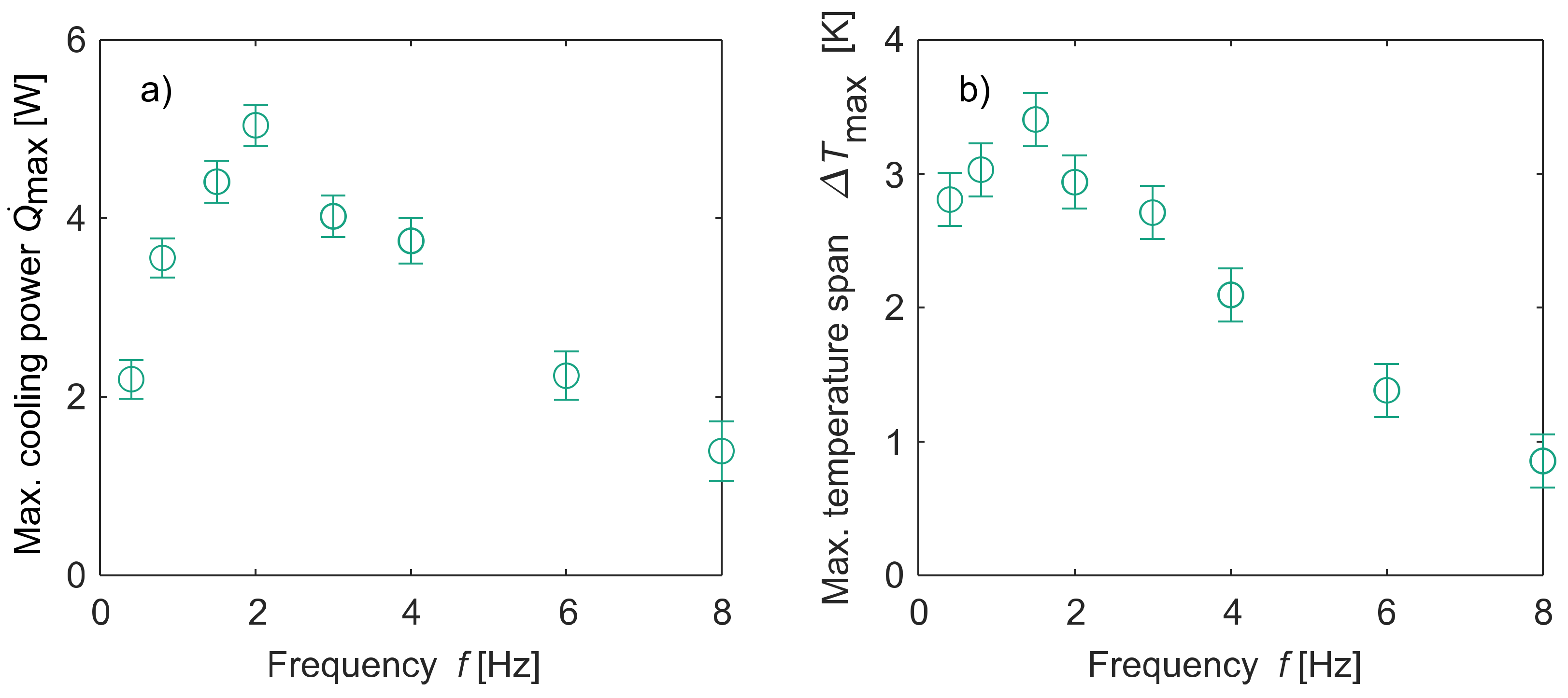
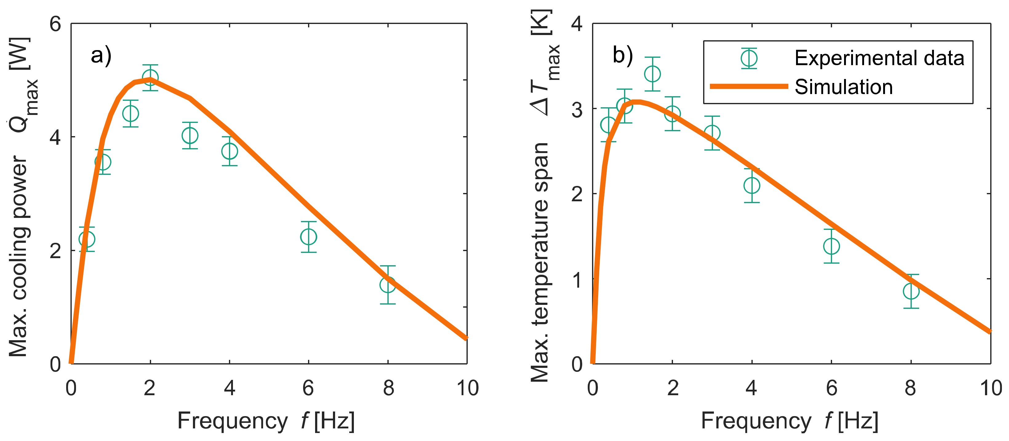
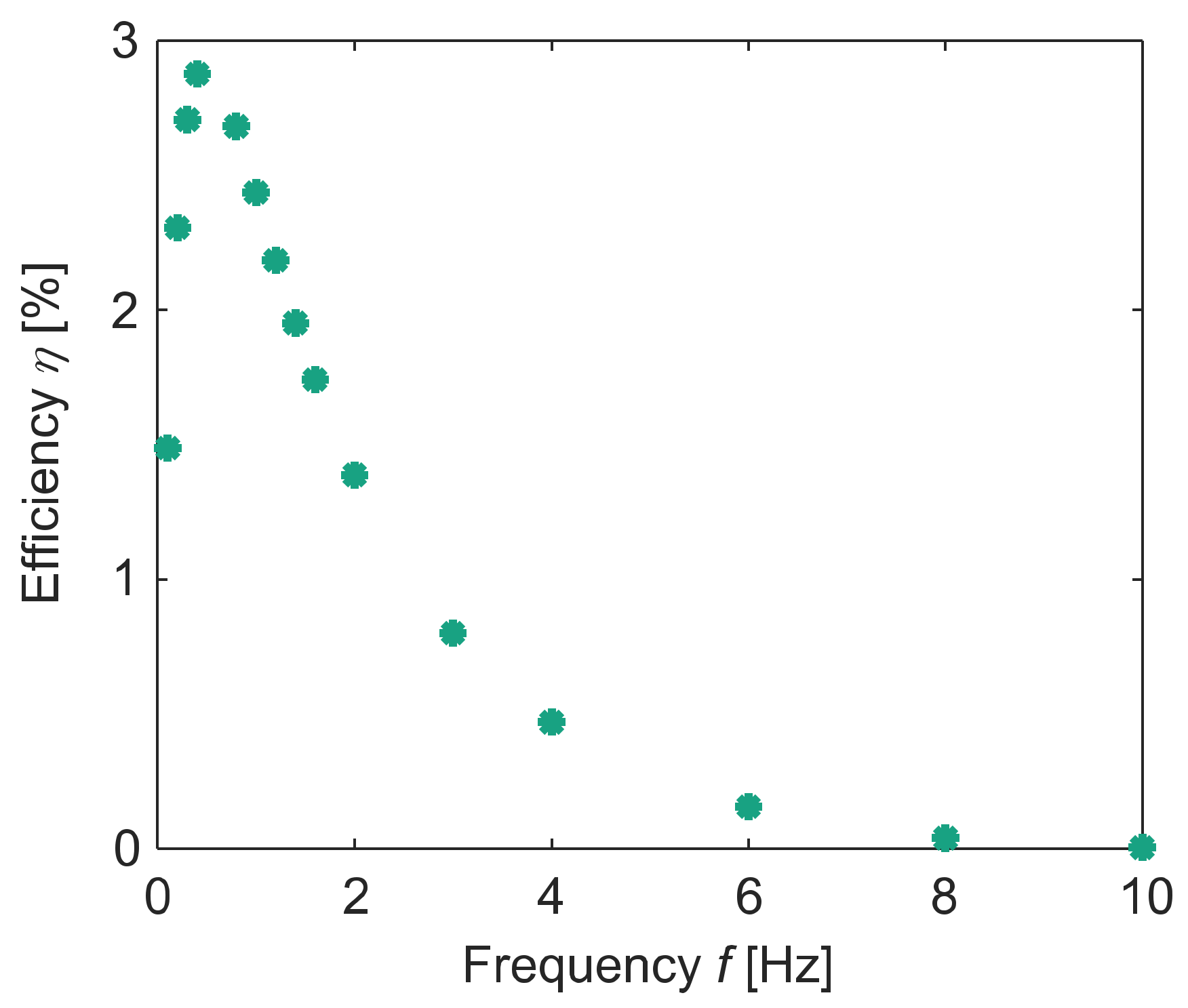
3.1. Experimental Data

The temperature span for different cooling powers is shown in Figure 5 for frequencies ranging from 0.4 Hz to 8 Hz. The maximum cooling power at a temperature span of 0 K was calculated by linear extrapolation between the temperature span and cooling power [26].
The maximum temperature span and cooling power in relation to frequency are shown in Figure 6. The maximum temperature span was achieved at 1.5 Hz and the maximum cooling power at 2 Hz. Due to the dissipative energy, the mean temperature of the ECM increased. Thereby, Δ T H increased and the temperature span Δ T as well as the cooling power decreased. This effect increased at high frequencies.

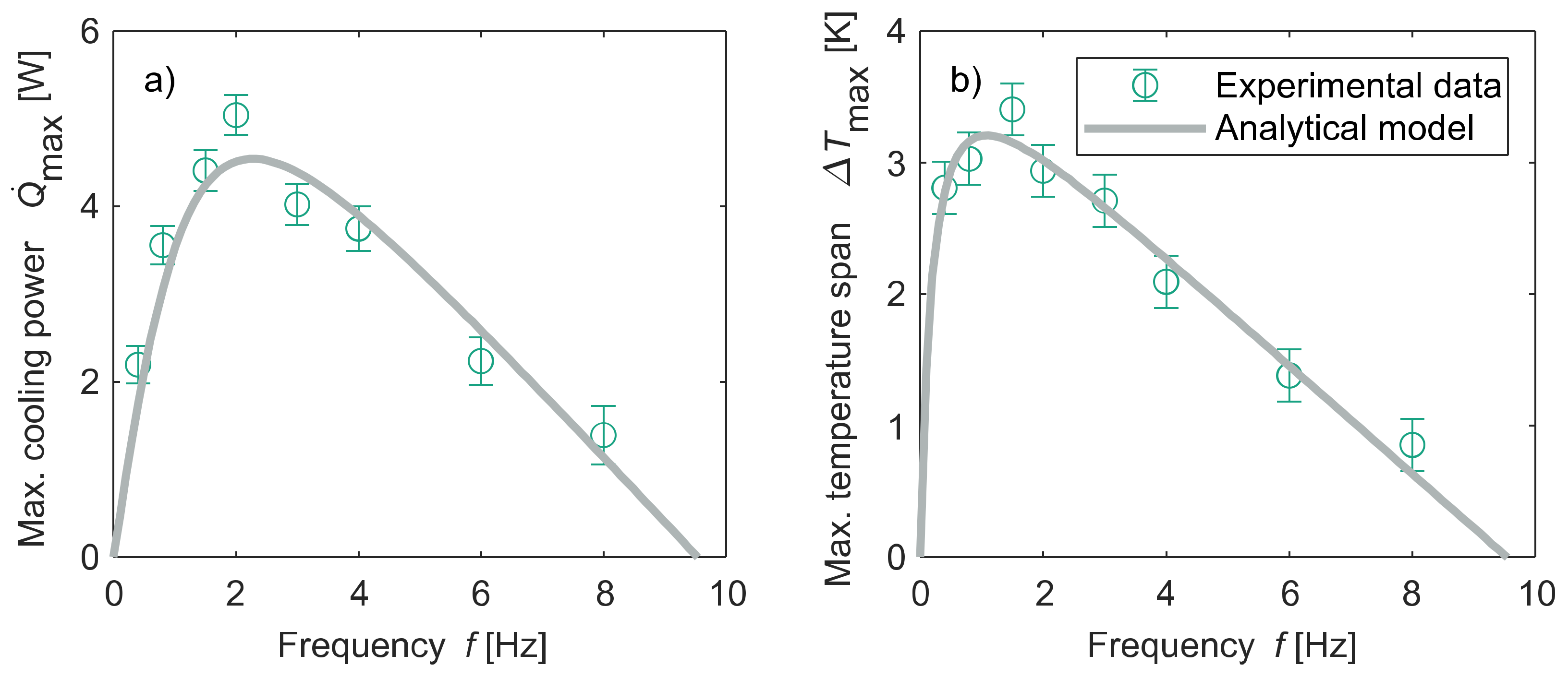
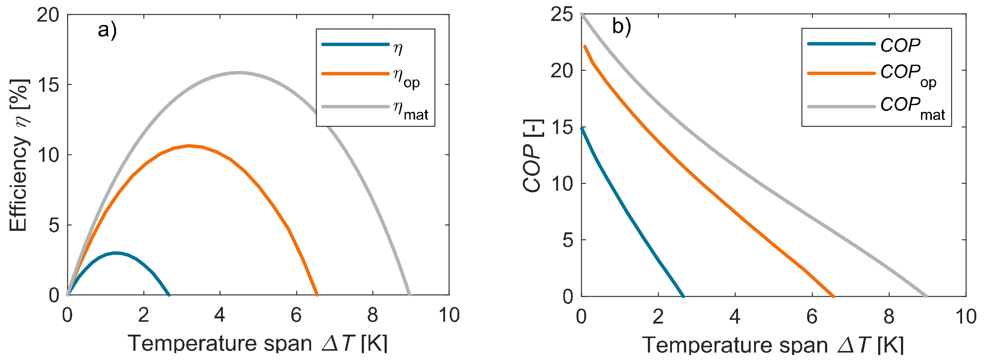
3.2. Results of the Analytical Evaluation

To determine parameters R Iso , R K , and R th , the equations for determining the maximum temperature span (Equation (6)) and the maximum cooling power (Equation (7)) were fitted simultaneously with a least square method to the measured values, which resulted in R K = (1.22 ± 0.06) K/W, R th = (0.099 ± 0.006) K/W, and R Iso = (4.5 ± 0.9) K/W. The standard deviations resulted from entries of the main diagonal of the covariance matrix during fitting. The simplified analytical model, shown with the measurement data in Figure 7, accurately depicts the experimental data.

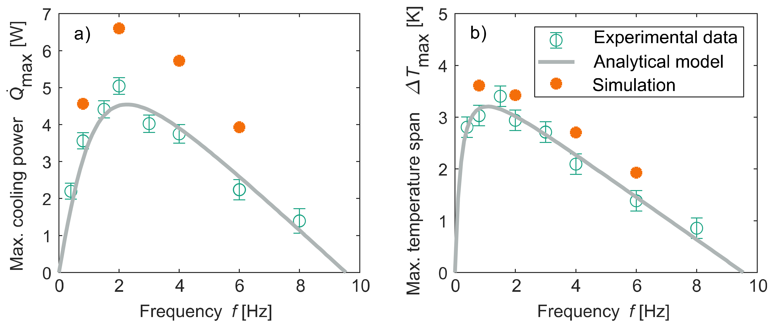
3.3. Results of the Simulation

The thermal resistances determined in the simplified analytical model were used as a starting point in the Simscape model. Figure 8 shows the analytical model and the simulation of the AEH for individual frequencies. The results from the time-dependent two-phase system simulations deviated from those in the simplified analytical model, which was fitted to the measurement data. This is partly because the analytical model does not take into account the nonlinear behavior of the ECM. Moreover, the time-dependency of the material behavior is not considered. The simplifications in the analytical model led to an underestimation in the temperature span and the cooling capacity compared to the simulation.
To reproduce the measured data with the simulation, we scaled the equations in the simplified analytic model and fitted the parameters again. This reduced R th and increased R Iso . The parameters R K = (1.18 ± 0.04) K/W, R th = (0.168 ± 0.002) K/W, and R Iso = (2.8 ± 0.2) K/W were used in the simulation and verified with the measured data, as shown in Figure 9.

4. Discussion

The simulation can be used to calculate the efficiency of the AEH system. Therefore, the input power was calculated using the difference in heat fluxes flowing in and out of the system: P = Q ˙ R K + Q ˙ h Q ˙ in . The heat flux Q ˙ in corresponds to the cooling power.
The coefficient of performance COP as a function of the heat fluxes can be calculated using Equation (8):
C O P = Q ˙ in P
The coefficient of performance for a Carnot cycle without losses is determined using the temperature of the evaporator and the temperature span: C O P carnot = T c Δ T . The exergetic efficiency of the AEH is calculated as follows: η = C O P C O P carnot .
The exergetic efficiency of the material can be calculated using Equation (9), where a = Δ T Δ T ad applies [27]:
η mat 1 1 + 1 1 a a Δ T hys Δ T ad
The maximum material efficiency was reached at a = 0.5 and amounted to η mat = 16 % . The values for Δ T hys = 11.9 K and Δ T ad = 9.0 K were determined using the material model [24].
Figure 10 shows the maximum efficiency of the AEH in relation to the system frequency for Q ˙ max / 2 , which corresponds to Δ T / 2 due to the linear relationship between the temperature span and cooling power. The maximum efficiency was achieved at a frequency of 0.4 Hz. The heat that flows into the evaporator during a cycle increases at lower frequencies and reduces efficiency. Here, it can also be observed that at higher frequencies, dissipative heating causes the ECM to heat up, thus reducing the cooling power and efficiency.
Further simulations were carried out at a frequency of 0.4 Hz with the highest calculated efficiency level. Figure 11 shows a range of ideal scenarios in order to break down losses with respect to efficiency. Therefore, the maximum efficiency η max and the maximum temperature span Δ T max of the scenarios was plotted. The first two bars show the simulation of the experimental data. The scenario ’without insulations losses evaporator’ is without insulation losses in the evaporator. This results in an increase in the efficiency and the maximum temperature span. There was no resistance between the ECM and the fluid in the scenario ‘without heat transfer losses’. This modification results in an improvement in the efficiency. In steady state experiments, there is not enough fluid in the segment to transfer the dissipative heat of the ECM into the condenser. In the scenario ‘extra fluid’, additional fluid is on the surface of the ECM so that the ECM does not dry out. In this case, the mean temperature T m is below the temperature of the condenser. The efficiency and maximum temperature span increase in this scenario. The last column shows the simulation with extra fluid in the segment, so that the surface of the ECM does not dry out, and without insulation losses of the segment (‘extra fluid and without insulations losses segment’). These two aspects are presented in combination, because in simulations with a great R K and no additional fluid, the mean temperature of the ECM increases until the heat transfer collapses. The resistance of the insulation of the evaporator R Iso has the greatest impact on the maximal temperature span. The greatest efficiency is achieved by extra fluid and a high resistance R K .
The following section, however, strives to look at the extent to which efficiency can be improved by making realistic optimizations to the experimental setup. The resistance of the insulation between the evaporator and environment can theoretically be increased to R Iso = 33 K/W, in line with the principles of heat transfer by conduction through a tube [28], by using 10 cm polyethylene foam with a thermal conductivity of 0.04 W/(m K). The resistance between the ECM and the environment R K = 7.2 K/W can be achieved by using ceramics to thermally isolate the ECM from the environment.
By adjusting the sample geometry R th , the resistance between the ECM and the fluid can be reduced. This involves maximizing the surface of the ECM and reducing the wall thickness of the tube-shaped samples. The sample geometry was adapted in such a way that the samples neither failed due to the Euler buckling mode, nor due to buckling of the tube walls, and at the same time, the thermal resistance R th was minimized. According to the fourth Euler’s buckling mode, the critical stress is σ Euler = 4 π E I A l 2 [29]. Here, E is the Young’s modulus and the length of the samples is l . The area moment of inertia is I = π r a 4 r i 4 4 . r a and r i are the outer radius and the inner radius of the sample, respectively. A is the cross section of the sample. The critical stress for buckling due to the thin walls of the tube is given by σ buckling = E r a r i 4 r a A [30]. For the adaption of the thermal resistance, R th is assumed to be σ crit = σ Euler = σ buckling = 1000 MPa as the critical stress. The thermal resistance R th includes the resistance due to evaporation and condensation of the fluid and the heat conduction resistance in the ECM: R th = log r a log r i k 2 π l + 1 h 2 π r a l [31]. h = 7400 W/(m2K) was assumed as the heat transfer coefficient, which was calculated using the geometry data of the samples used in the experiments and the resistance R th from the analytical model. The thermal conductivity was k = 18 W/(mK) [32]. In this calculation, the mass and sample length were kept constant to remain the same as in the experiments. This resulted in a sample number of 195, which had an outer diameter of 0.8 mm and a wall thickness of 0.0375 mm. Through this optimization, the resistance between the ECM and the fluid can be reduced to 0.03 K/W.
In addition, the ECM was assumed to be only minimally wet to the extent that it does not dry out during the cycle and no excess fluid is on the surface of the ECM. This can be implemented in the AEH by recirculating liquid fluid from the condenser to the ECM passively by a wick. The fluid is distributed onto the ECM by structuring and coating the surface. This is one way to distribute additional fluid on the surface and counteract warming of the ECM.
A simulation performed using the optimized parameters (Figure 12a) with this system and these material properties resulted in an efficiency level of 10.4% at Δ T = 3.2 K, resulting in 67% of the material efficiency. Figure 12b shows the C O P of the AEH compared with the C O P op with optimized parameters and that of the material C O P mat . Both figures also show the increase in the maximum temperature span from 2.7 K to 6.5 K.

5. Conclusions

Using an analytical model, we determined the thermal resistances to simulate the active elastocaloric heat pipe. This simulation can be used to model system behavior, determine non-measurable variables such as heat fluxes, and on this basis, calculate the system’s efficiency levels. The loss mechanisms such as efficiency losses caused by the material, non-ideal isolation of the evaporator, and resistance caused by thermal conduction in the ECM were examined individually to determine their effect on the system efficiency. By improving the system parameters to the extent technically possible, an efficiency increase to 67% of the material efficiency could be achieved. These simulation results can be used to determine measures to improve the system performance and implement such measures in future structures.

Author Contributions

Conceptualization, N.B. and K.B.; Formal analysis, N.B. and D.S.; Funding acquisition, O.S.-W.; Methodology, N.B. and K.B.; Project administration, K.B.; Software, N.B., D.S. and K.B.; Supervision, T.K. and K.B.; Validation, N.B. and D.B.; Visualization, N.B.; Writing–original draft, N.B.; Writing–review & editing, N.B. and K.B. All authors have read and agreed to the published version of the manuscript.

Funding

This research was funded by Federal Ministry of Education and Research (BMBF), grant number 03VP04670.

Institutional Review Board Statement

Not applicable.

Informed Consent Statement

Not applicable.

Data Availability Statement

All data presented and discussed in this study are represented in the figures shown in this work, and thus are publicly available.

Conflicts of Interest

The authors declare no conflict of interest.

Nomenclature

Roman symbols
a Working point variable, -
A Area, m2
c Specific heat capacity, J kg−1 K−1
c 0 Specific baseline heat capacity, J kg−1 K−1
C O P Coefficient of performance, -
E Young’s modulus, MPa
f Frequency, Hz
f c Cut-off frequency, Hz
h Heat transfer coefficient, W m−2 K−1
I Area moment of inertia, m4
k Thermal conductivity, W m−1 K−1
l Length, m
m Mass, kg
P Power, W
q Specific heat, J kg−1
Q ˙ Heat flux, W
r Radius, m
R Thermal resistance, K W−1
R iso Insulation resistance of the evaporator, K W−1
R K Insulation resistance between the ECM and the environment, K W−1
R th Resistance between ECM and fluid, K W−1
s Specific entropy, J kg−1 K−1
T Temperature, K
T 0 Peak temperature, K
Greek symbols
α Half wide at half maximum of the peak, K
β Multiplicative inverse of the Clausius-Clapeyron coefficient, K MPa−1
Δ Finite difference, -
η Exergetic efficiency, -
σ Stress, MPa
Subscripts
aOuter
AAmbient
adAdiabatic
bucklingCritical buckling
cCold side
carnotCarnot cycle
diss Dissipative
ECM Elastocaloric material
effEffective
EulerEuler‘s buckling mode
hHot side
HAverage warming in relation to the environment and condenser
hysHysteresis
IInner
inInto the evaporator
isoIsothermal
mMean
matMaterial
maxMaximal
opOptimized
pFor pumping of the heat
R iso Insulation resistance of the evaporator
R K Insulation resistance between the ECM and the environment
R th Resistance between ECM and fluid

References

  1. International Energy Agency. The Future of Cooling: Opportunities for Energy-Efficient Air Conditioning. 2018. Available online: https://www.iea.org/reports/the-future-of-cooling (accessed on 2 January 2022).
  2. Goetzler, W.; Zogg, R.; Young, J.; Johnson, C. Energy Savings Potential and RD&D Opportunities for Non-Vapor-Compression HVAC Technologies; prepared for US Department of Energy; Navigant Consulting Inc.: Chicago, IL, USA, 2014. [Google Scholar]
  3. Kitanovski, A.; Tušek, J.; Tomc, U.; Plaznik, U.; Ožbolt, M.; Poredoš, A. Magnetocaloric Energy Conversion: From Theory to Applications; Springer: Cham, Switzerland, 2015; ISBN 978-3-319-08740-5. [Google Scholar]
  4. Ossmer, H.; Chluba, C.; Kauffmann-Weiss, S.; Quandt, E.; Kohl, M. TiNi-based films for elastocaloric microcooling—Fatigue life and device performance. APL Mater. 2016, 4, 64102. [Google Scholar] [CrossRef]
  5. Bruederlin, F.; Ossmer, H.; Wendler, F.; Miyazaki, S.; Kohl, M. SMA foil-based elastocaloric cooling: From material behavior to device engineering. J. Phys. D Appl. Phys. 2017, 50, 424003. [Google Scholar] [CrossRef]
  6. Schmidt, M.; Schuetze, A.; Seelecke, S. Scientific test setup for investigation of shape memory alloy based elastocaloric cooling processes. Int. J. Refrig. 2015, 54, 88–97. [Google Scholar] [CrossRef]
  7. Ulpiani, G.; Bruederlin, F.; Weidemann, R.; Ranzi, G.; Santamouris, M.; Kohl, M. Upscaling of SMA film-based elastocaloric cooling. Appl. Therm. Eng. 2020, 180, 115867. [Google Scholar] [CrossRef]
  8. Chen, Y.; Wang, Y.; Sun, W.; Qian, S.; Liu, J. A compact elastocaloric refrigerator. Innovation 2022, 3, 100205. [Google Scholar] [CrossRef] [PubMed]
  9. Snodgrass, R.; Erickson, D. A multistage elastocaloric refrigerator and heat pump with 28 K temperature span. Sci. Rep. 2019, 9, 18532. [Google Scholar] [CrossRef] [PubMed]
  10. Kirsch, S.-M.; Welsch, F.; Michaelis, N.; Schmidt, M.; Wieczorek, A.; Frenzel, J.; Eggeler, G.; Schütze, A.; Seelecke, S. NiTi-Based Elastocaloric Cooling on the Macroscale: From Basic Concepts to Realization. Energy Technol. 2018, 6, 1567–1587. [Google Scholar] [CrossRef]
  11. Engelbrecht, K.; Tušek, J.; Eriksen, D.; Lei, T.; Lee, C.-Y.; Tušek, J.; Pryds, N. A regenerative elastocaloric device: Experimental results. J. Phys. D Appl. Phys. 2017, 50, 424006. [Google Scholar] [CrossRef] [Green Version]
  12. Tušek, J.; Engelbrecht, K.; Eriksen, D.; Dall’Olio, S.; Tušek, J.; Pryds, N. A regenerative elastocaloric heat pump. Nat. Energy 2016, 1, 10. [Google Scholar] [CrossRef]
  13. Qian, S.; Geng, Y.; Wang, Y.; Muehlbauer, J.; Ling, J.; Hwang, Y.; Radermacher, R.; Takeuchi, I. Design of a hydraulically driven compressive elastocaloric cooling system. Sci. Technol. Built Environ. 2016, 22, 500–506. [Google Scholar] [CrossRef]
  14. Michaelis, N.; Kirsch, S.-M.; Welsch, F.; Rizello, G.; Seelecke, S.; Motzki, P. Investigation of Elastocaloric Air Cooling Potential Based on Superelastic SMA Wire Bundles. Available online: https://www.researchgate.net/publication/344198524_INVESTIGATION_OF_ELASTOCALORIC_AIR_COOLING_POTENTIAL_BASED_ON_SUPERELASTIC_SMA_WIRE_BUNDLES (accessed on 1 July 2021).
  15. Cheng, S.; Xiao, Y.; Li, X.; Lin, H.; Hua, P.; Sheng, L. Buckling Prevention of a Single Long NiTi Tube Compressive Elastocaloric Regenerator; SSRN: Rochester, NY, USA, 2022. [Google Scholar] [CrossRef]
  16. Zhang, J.; Zhu, Y.; Cheng, S.; Yao, S.; Sun, Q. Enhancing cooling performance of NiTi elastocaloric tube refrigerant via internal grooving. Appl. Therm. Eng. 2022, 213, 118657. [Google Scholar] [CrossRef]
  17. Ianniciello, L.; Bartholomé, K.; Fitger, A.; Engelbrecht, K. Long life elastocaloric regenerator operating under compression. Appl. Therm. Eng. 2022, 202, 117838. [Google Scholar] [CrossRef]
  18. Sharar, D.J.; Radice, J.; Warzoha, R.; Hanrahan, B.; Chang, B. First Demonstration of a Bending-Mode Elastocaloric Cooling ‘Loop’. In Proceedings of the 2018 17th IEEE InterSociety Conference on Thermal and Thermomechanical Phenomena in Electronic Systems, ITherm 2018, San Diego, CA, USA, 29 May–1 June 2018; IEEE: Piscataway, NJ, USA, 2018; pp. 218–226, ISBN 978-1-5386-1272-9. [Google Scholar]
  19. Bachmann, N.; Fitger, A.; Maier, L.M.; Mahlke, A.; Schäfer-Welsen, O.; Koch, T.; Bartholomé, K. Long-term stable compressive elastocaloric cooling system with latent heat transfer. Commun. Phys. 2021, 4, 615. [Google Scholar] [CrossRef]
  20. Welsch, F.; Kirsch, S.-M.; Michaelis, N.; Mandolino, M.; Schütze, A.; Seelecke, S.; Motzki, P.; Rizzello, G. System Simulation of an Elastocaloric Heating and Cooling Device Based on SMA. In Proceedings of the ASME 2020 Conference on Smart Materials, Adaptive Structures and Intelligent Systems, Virtual, Online, 15 September 2020; American Society of Mechanical Engineers: New York, NY, USA, 2020; Volume 09152020. [Google Scholar]
  21. Cheng, S.; Xiao, Y.; Li, X.; Lin, H.; Hua, P.; Sheng, L.; Sun, Q. Elastocaloric Effect Characterization of a NiTi Tube to be Applied in a Compressive Cooling Device; SSRN: Rochester, NY, USA, 2022. [Google Scholar]
  22. Bruederlin, F.; Bumke, L.; Chluba, C.; Ossmer, H.; Quandt, E.; Kohl, M. Elastocaloric Cooling on the Miniature Scale: A Review on Materials and Device Engineering. Energy Technol. 2018, 6, 1588–1604. [Google Scholar] [CrossRef]
  23. Qian, S.; Alabdulkarem, A.; Ling, J.; Muehlbauer, J.; Hwang, Y.; Radermacher, R.; Takeuchi, I. Performance enhancement of a compressive thermoelastic cooling system using multi-objective optimization and novel designs. Int. J. Refrig. 2015, 57, 62–76. [Google Scholar] [CrossRef] [Green Version]
  24. Bachmann, N.; Fitger, A.; Unmüßig, S.; Bach, D.; Schäfer-Welsen, O.; Koch, T.; Bartholomé, K. Phenomenological model for first-order elastocaloric materials. Int. J. Refrig. 2022, 136, 245–253. [Google Scholar] [CrossRef]
  25. Maier, L.M.; Hess, T.; Kaube, A.; Corhan, P.; Fitger, A.; Bachmann, N.; Schäfer-Welsen, O.; Wöllenstein, J.; Bartholomé, K. Method to characterize a thermal diode in saturated steam atmosphere. Rev. Sci. Instrum. 2020, 91, 65104. [Google Scholar] [CrossRef] [PubMed]
  26. Hess, T.; Maier, L.M.; Corhan, P.; Schäfer–Welsen, O.; Wöllenstein, J.; Bartholomé, K. Modelling cascaded caloric refrigeration systems that are based on thermal diodes or switches. Int. J. Refrig. 2019, 103, 215–222. [Google Scholar] [CrossRef]
  27. Hess, T.; Maier, L.M.; Bachmann, N.; Corhan, P.; Schäfer-Welsen, O.; Wöllenstein, J.; Bartholomé, K. Thermal hysteresis and its impact on the efficiency of first-order caloric materials. J. Appl. Phys. 2020, 127, 75103. [Google Scholar] [CrossRef]
  28. Baehr, H.D.; Stephan, K. Wärme- und Stoffübertragung; Springer: Berlin/Heidelberg, Germany, 2019; ISBN 978-3-662-58440-8. [Google Scholar]
  29. Lackmann, J.; Mertens, H.; Liebich, R. Stabilitätsprobleme. In Dubbel: Taschenbuch für den Maschinenbau; Grote, K.-H., Feldhusen, J., Eds.; Springer: Berlin/Heidelberg, Germany, 2011; pp. C42–C46. ISBN 978-3-642-17306-6. [Google Scholar]
  30. Altenbach, H. Technische Mechanik Festigkeitslehre; Springer Fachmedien: Wiesbaden, Germany, 2018; ISBN 978-3-658-22853-8. [Google Scholar]
  31. Verein Deutscher Ingenieure. VDI Heat Atlas, 2nd ed.; Springer: Berlin/Heidelberg, Germany, 2010; ISBN 978-3-540-77876-9. [Google Scholar]
  32. Ordonez-Miranda, J.; Hill, J.M.; Joulain, K.; Ezzahri, Y.; Drevillon, J. Conductive thermal diode based on the thermal hysteresis of VO2 and nitinol. J. Appl. Phys. 2018, 123, 85102. [Google Scholar] [CrossRef]
Figure 1. The AEH concept with one segment in four consecutive time steps [19]: (I) A load is applied to the ECM, causing it to heat up. The fluid on the surface evaporates. (II) The pressure in this segment increases, causing the right valve to open and steam to flow into the condenser. (III) When the load is removed from the ECM, it cools down. (IV) The pressure in the chamber decreases to a level below the pressure in the previous segment, causing the left valve to open and steam to flow from the evaporator into the segment and condense on the ECM.
Energies 15 05089 g001
Figure 2. Schema of the simulation. Thermal data are shown in red and fluid data in blue. The evaporator has the temperature T c and is connected to the environment via the thermal resistance R Iso representing the insulation. The heat flux Q ˙ R Iso flows into the evaporator via this resistance. The cooling power is measured on the basis of the heat flux Q ˙ in . The evaporator is connected to the segment by a check valve. Here, the ECM is compressed along a sinusoidal stress profile. The ECM is connected to the environment via the thermal resistance R K and the heat flux Q ˙ R K . The ECM is connected to the fluid via R th . The heat flux at this resistance is Q ˙ R th . The fluid flows from the segment into the condenser at temperature T h . From the condenser, the heat flux Q ˙ h is dissipated into the environment. The fluid flows back into the evaporator through a throttle. The temperature span of the AEH is Δ T = T h T c .
Energies 15 05089 g002
Figure 3. The simulation of the check valve and data [25] of the volume flow for the differential pressure.
Energies 15 05089 g003
Figure 4. The temperatures for the analytical model from a stationary perspective: Δ T ad 2 is made up of Δ T H , the difference in temperature compared with the environment; Δ T , the temperature span of the AEH; and Δ T p , the temperature span for pumping heat.
Energies 15 05089 g004
Figure 5. The temperature span between the evaporator (heat source) and the temperature-controlled condenser (heat sink) in relation to the cooling power applied for different frequencies. The maximum cooling power at a temperature span of 0 K can be deduced by means of linear extrapolation. (a) Frequencies from 0.4 Hz to 2 Hz. (b) Frequencies from 3 Hz to 8 Hz.
Energies 15 05089 g005
Figure 6. (a) shows the maximum cooling power of the AEH for different frequencies. (b) The maximum temperature span of the AEH for different frequencies.
Energies 15 05089 g006
Figure 7. Measurement data and analytical model. (a) The maximum cooling power and (b) the maximum temperature span in relation to frequency.
Energies 15 05089 g007
Figure 8. The analytical model and time dependent simulation of the measurement data pertaining to the maximum cooling power (a) and maximum temperature span (b). The simulation overestimated the measurement data, while the model depicts them accurately.
Energies 15 05089 g008
Figure 9. The results of the simulation compared with the measurement data pertaining to the maximum cooling power (a) and the maximum temperature span (b).
Energies 15 05089 g009
Figure 10. Efficiency of the AEH η at Q ˙ max / 2 in relation to the system frequency.
Energies 15 05089 g010
Figure 11. The maximum efficiency and maximum temperature span for different scenarios. The simulation of the experiment on the left is given as a reference. In the scenario ’without insulations losses evaporator’, no insolation losses in the evaporator are assumed. ‘Without heat transfer losses’ represents a scenario where there is no resistance between the ECM and the fluid. In the scenario ‘extra fluid’, additional fluid is assumed to be on the surface of the ECM. The last column shows a scenario with ‘extra fluid and without insulations losses segment’ and no insulation losses in the segment.
Energies 15 05089 g011
Figure 12. Simulation of the efficiency with improved system parameters. (a) The efficiency of the optimized system η op compared with the efficiency of the AEH of η . The optimized system achieved 67% of the material efficiency η mat . (b) The C O P of the AEH compared with the C O P op with optimized parameters and that of the material C O P mat .
Energies 15 05089 g012
Publisher’s Note: MDPI stays neutral with regard to jurisdictional claims in published maps and institutional affiliations.

