Article

Deep-XFCT: Deep Learning 3D-Mineral Liberation Analysis with Micro-X-ray Fluorescence and Computed Tomography

1
Tyree X-ray CT Facility, Mark Wainwright Analytical Centre, UNSW Sydney, Sydney, NSW 2052, Australia
2
School of Minerals and Energy Resources Engineering, UNSW Sydney, Sydney, NSW 2052, Australia
3
Mark Wainwright Analytical Centre, UNSW Sydney, Sydney, NSW 2052, Australia
4
Western Australian School of Mines, Curtin University, Bentley, WA 6102, Australia
*
Author to whom correspondence should be addressed.
Energies 2022, 15(15), 5326; https://doi.org/10.3390/en15155326
Submission received: 31 May 2022 / Revised: 18 July 2022 / Accepted: 19 July 2022 / Published: 22 July 2022
(This article belongs to the Special Issue Application of Machine Learning in Rock Characterization)

Abstract

:
Quantitative characterisation through mineral liberation analysis is required for effective minerals processing in areas such as mineral deposits, tailings and reservoirs in industries for resources, environment and materials science. Current practices in mineral liberation analysis are based on 2D representations, leading to systematic errors in the extrapolation to 3D volumetric properties. The rapid development of X-ray microcomputed tomography (μCT) opens new opportunities for 3D analysis of features such as particle- and grain-size characterisation, determination of particle densities and shape factors, estimation of mineral associations, and liberation and locking. To date, no simple non-destructive method exists for 3D mineral liberation analysis. We present a new development based on combining μCT with micro-X-ray fluorescence (μXRF) using deep learning. We demonstrate successful semi-automated multimodal analysis of a crystalline magmatic rock by obtaining 2D μXRF mineral maps from the top and bottom of the cylindrical core and propagating that information through the 3D μCT volume with deep learning segmentation. The deep learning model was able to segment the core to obtain reasonable mineral attributes. Additionally, the model overcame the challenge of differentiating minerals with similar densities in μCT, which would not be possible with conventional segmentation methods. The approach is universal and can be extended to any multimodal and multi-instrument analysis for further refinement. We conclude that the combination of μCT and μXRF can provide a new opportunity for robust 3D mineral liberation analysis in both field and laboratory applications.

1. Introduction

To determine the volume fractions of valuable commodities, mineral liberation has become a key step in the mineral processing industry, whereby through the process of breaking up the ore, valuable minerals are released for separation [1]. Mineral liberation analysis is therefore frequently used in metallurgical and mineralogical application for mineral abundance estimation in modal mineralogy and assay techniques for sample elemental distributions [2]. Mineral liberation analysis has also been used in research and industry for particle- and grain-size characterisation [3], determination of particle densities and shape factors [4], estimation of mineral associations, liberation and locking [5] and theoretical grade–recovery curves [6]. The technique has now been extended for characterisation of ore deposits to secondary resource characterisation of tailings [7], and applications in the petroleum industry for the characterisation of sediments [8], rock typing, stratigraphic refinement and reservoir characterisation [9].
Several semi-automated techniques have been developed for identifying and quantifying mineralogy. Of widest use are currently electron-beam-based systems using backscattered electron (BSE) images with energy-dispersive spectroscopy (EDS) marketed as commercial systems such as QEMSCAN [10,11]. However, the extrapolation of the collected 2D mineralogy maps to 3D remains problematic. The current methods of stereological reconstruction, at present, cannot solve the difficult mathematical problem of the diversity and complexity of mineral grains in rocks and ores due to the difficult-to-define form factor. This leads to systematic errors in quantitative estimates of volume fractions from 2D data as input into mass–energy balance calculations in mineral processing flow sheets [12]. To rigorously address this problem, 3D tomographic imaging techniques are necessary.
Destructive tomographic methods, such as focused ion beam milling coupled with high-resolution scanning electron microscope (FIB-SEM) imaging, offer exact 3D reconstructions down to the nanometre level and can be complemented by SEM/EDX automated mineralogy [13] on 2D cross-sections. Recent developments in X-ray microcomputed tomography (μCT) have made rapid non-destructive characterisation possible, and the technique has now been successfully integrated into the SEM/EDX-based mineral liberation analysis [14]. Furthermore, studies have combined micro-X-ray fluorescence (μXRF) with μCT [15] in addition to implementations of artificial intelligence being explored for straightforward segmentations of 2D μXRF maps of rocks [16].
The question arises regarding whether a technique can be successfully developed where the exterior surface mineralogy can be combined with the interior bulk of a 3D X-ray μCT dataset for direct, fast and reliable 3D mineral liberation analysis. The problem is the densities of some geomaterials are so similar that without additional information, it is difficult and, often, impossible to reliably differentiate between distinct phases in X-ray μCT. This problem is encountered when trying to identify feldspar crystals from crystallised natural magmas where specialised image analysis techniques have been proposed to augment the analysis of tomographic slices through morphological information of feldspar crystals [17]. However, artificial intelligence, through deep learning protocols, have been found to be useful in overcoming many of the hurdles mentioned in the segmentation of materials [18,19,20]. Additionally, the advent of machine learning has enhanced numerous aspects of mineral processing [21]. Applications include the prediction of coal flotation performance [22,23,24], power consumption optimisations [25,26] and grinding burn detection [27], all of which warrant further development of machine learning in mineral characterisation.
Our hypothesis is an envisioned workflow that can be generalised by artificial intelligence techniques and is able to incorporate additional information, such as statistical analysis, into a robust 3D mineral liberation analysis technique using laboratory equipment. In this contribution, we propose a generic multi-instrument, multimodal analysis technique by combining a deep learning approach and statistical methods for interpretating X-ray μCT and μXRF images, called deep X-ray florescence computed tomography (Deep-XFCT). Our aim was to reliably identify and resolve the shapes and distribution of the mineral phases with minor density differences, which will have an effect on mineral flotation as well as the energy needed for rock breakage (comminution); one of the most energy-intensive processes in mining [28].

2. Methods

2.1. Core Plug Rock Sample

Multimineral Rock Sample

The basaltic andesite core plug sample used in this study was obtained from the NSW Government Londonderry core library. The rock was subdrilled from a 45 mm round rock collection of the Pacific Power Hot Rock 1 bore (PPHR1). The rock was originally from the Muswellbrook geothermal anomaly, located approximately 10 km southwest of Muswellbrook in Hunter Valley Dome Belt, the north-eastern part of the Sydney basin, New South Wales. The PPHR1 borehole was drilled to a depth of 1946 m near the central region of the anomaly, and more than 1 km of continuous core samples was taken to identify the rocks present and their physical properties [29].
The basaltic andesite sample was a fine-grained igneous rock with a silica content from 52% to 57% [30]. The sample was chosen for its clear and distinct mineral inclusions, which are preferable for application in a proof-of-concept workflow. The initial drill core analysed had a diameter of 24.30 mm and height of 25 mm. Sample preparation for the analysis was minimal with the drill core sample. The sample was simply cut orthogonal to the length of the cylindrical core with a Struers® Minitom to obtain a relatively flat surface, with no polishing performed for the surface.

2.2. Experimental Methods

To obtain 3D mineral liberation of the basaltic andesite sample, a combination of conventional analytical techniques was employed for analysis and validation. These included (1) XRD on powder samples of the rock to gain an understanding of the minerals present and their relative abundances; (2) μCT for a 3D representation of the densities of the mineral, as shown in Figure 1; (3) μXRF for point analysis of elemental atomic mass, shown in Figure 2, and to obtain the elemental concentration maps from the top and bottom surfaces of the sample, as shown in Figure 3; (4) Raman scattering to validate several mineral phases from the current workflow. The XRD and Raman scattering data, along with detailed specifications of the experimental methods can be found in the Supplementary Materials.

2.2.1. Powder X-ray Diffraction (XRD)

The XRD was performed to identify the general mineralogy of the rock. A powder specimen was prepared by the backloading method, where random fractions of the rock sample were crushed into powder and sieved to reach a particle size of less than 300 mesh B.S. The powder was dried inside an oven at 50 °C for 24 h. The data were collected using an Empyrean XRD (PANalytical, Almelo, The Netherlands) fitted with Co as an anode at 45 kV and 40 mA at the Mark Wainwright Analytical Centre, University of New South Wales (UNSW), Sydney. The collected data were processed by the High Score Plus software (PANalytical, Almelo, The Netherlands). A search for a match with the candidate’s crystalline phase was performed using the PDF 4+ database, followed by Rietveld refinement to quantify the crystalline mineral phases. The resulting mineral phases extracted are shown in Table 1. The data and the Rietveld refinement can be found in the Supplementary Materials.

2.2.2. Microcomputed Tomography (μCT)

The μCT imaging was performed using the Heliscan μCT system at the Tyree X-ray μCT Facility at the University of New South Wales. The Tyree Heliscan μCT has a General Electric Phoenix Nanofocus tube with a diamond window, a high-quality flatbed detector (3072 × 3072 pixels, 3.75 fps readout rate). The facility was built in a lead-lined room with temperature and humidity control (∆T < 0.5 °C). The samples were scanned in a helical trajectory with the following setting: 100 kV, 130 µA (tube current), exposure time 0.71 s, 5 accumulations, 0.5 mm stainless steel, 0.75 mm aluminium filter and 2880 projections over a 360° revolution. The voxel size obtained from this sample was 10.79 µm. The tomographic reconstruction was performed using the QMango software. The resulting tomogram of the sample is shown in Figure 1.

2.2.3. Micro-X-ray Fluorescence (μXRF)

The purpose of μXRF was to provide mineral labels for the μCT data and the atomic mass percentages of discrete points for mineral verification. The plug was cut into a cylindrical shape to ensure that there were two flat surfaces on the top and bottom of the cylinder to obtain μXRF maps, as shown in Figure 1. The μXRF mapping was carried out on a benchtop M4 Tornado μXRF (Bruker, Germany) under vacuum condition (20 mbar). The instrument consisted of a Rh anode metal–ceramic X-ray tube. A voltage of 45 kV and a current of 600 μA were used. X-ray spot calibration was carried out by digital tuning of the X-ray position indicated on the screen to align with the physical position on the sample. One silicon drift detector was used to count the fluorescent X-rays with an energy resolution ≤ 145 eV at full width half maximum for Mn-Kα.
For elemental mapping analysis, a spot size of 20 μm was used and the resulting spectra were acquired every 40 μm with an acquisition time of 200 ms/pixel. Data processing was performed using the M4 Tornado built-in software, FP MQuant (Bruker, Germany) for peak identification and quantification. The data collected from the μXRF maps were XRF intensities, which were normalised 8 bit values for all of the elements analysed. This gave relative elemental concentrations across the whole surface, which provided a semiquantitative measure (Figure 3). In addition to the μXRF maps obtained for the complete surfaces of the sample, points of interest of size 20 μm were collected (Figure 2) to obtain mass percentages as a further form of quantitative validation.

2.2.4. Raman Spectroscopy

Specific points were selected based on the mineral phases that were identified from the μXRF maps to confirm the minerals determined through μXRF. Raman spectroscopy was performed using an inVia Raman microspectrometer (Renishaw, UK) with a 532 nm excitation source. Raman spectra were recorded in the static mode centred at 1015 cm−1 (measurement range: 61–1839 cm−1) with a 20× objective, 100% laser power (approximately 33 mW at the sample), 1 s exposure and 100 accumulations. Spectra were processed using WiRE software (Version 5.3, Renishaw, UK) and baseline-corrected to remove the fluorescent background. Spectra were compared to known standards from the online RRUFF database using the phases determined by XRD [31].

2.3. Data Analytical Methods

The general workflow of the analytical process can be summed in two overarching steps: (1) establish ground truth labelling of the mineral phases on the top and bottom of the cylindrical sample through μXRF elemental mapping using K-means clustering; (2) use the ground truth labelling of the two surfaces to train a deep learning model that will segment the mineral phases in 3D μCT data. The K-means clustering was performed through the Scikit-learn library [32], and the remaining data analytical procedures and visualisations were performed with Dragonfly ORS, including the deep learning segmentation with the Segmentation Wizard [33].

2.3.1. Establishing the Training Data

To train the deep segmentation learning model to recognise mineral phases based on the μCT attenuation data, a training dataset needs to be established. Here, the training data were 2D images of the mineral phases obtained from μXRF elemental mapping. Not all element maps were used, but the ones used were chosen based on the major elements identified through XRD. For this basaltic andesite sample, the major elements present were Al, Ca, Fe, K, Mg, Mn, Na and Si. The μXRF element maps for the bottom surface are shown in Figure 3, and all remaining maps from all surfaces collected can be found in the Supplementary Materials.

K-Means Clustering

K-means clustering was used to automate the identification of mineral phases through the unique information from each elemental map to form the training data for the segmentation model. By grouping the XRF concentration intensities from different elements into a predefined number of clusters, their clustering centroids serve as a representation of the cluster. This is a fast and simple method that has been shown to extract mineral phases from μXRF maps [16]. Prior to performing the K-means clustering with all μXRF elements, some μXRF maps required preprocessing. This was performed for the μXRF maps with low atomic numbers, such as Na and Mg, where the XRF signals were relatively low and resulted in elemental maps with significant noise as shown in Figure 4. To address the issue of noise, various denoising filters can be used. For the specific aim of separating different areas to define minerals, a bilateral filter was used [34]. Bilateral filtering is particularly effective for the application of mineral identification in rocks, as it results in homogenous regions of elemental intensity while maintaining the edges between such regions. The identification of such edges is important for a well-defined dataset to train an effective deep learning segmentation model.
Seven clusters were used based on the six minerals, recognised from XRD, and the background void. The input data were from μXRF 8 bit images from Al, Ca, Fe, K, Mg, Mn, Na and Si. Along with these eight μXRF images, the appropriate orthoslice in the μCT data was also used in the K-means clustering as shown in Figure 2. This was done to provide added statistical weighting to the greyscale intensities of the μCT images that would be labelled as a result of the clustering. The μCT images were prepared by normalising the original μCT orthoslice to 8-bit values and resampling the μCT image with approximately 10 μm pixels into the geometry of the μXRF images with 40 μm pixels using cubic interpolation
Following the preprocessing of the Na and Mg μXRF maps, K-means clustering was applied to segment minerals by combining all eight relevant elemental maps and the corresponding μCT orthoslice, with each image serving as a dimension in the clustering space. The clustering was performed through the Scikit-learn Python library [32], where the best output in terms of inertia from 10 random initial clustering centroids was taken. The final centroids output represented the minerals and were used as labels for training the deep learning segmentation model (Table 2).

Image Registration

To perform the registration of the 2D mineral image from the K-means clustering analysis to the X-ray μCT volume, a μXRF image with high contrast and similar structures evident was used. In this case, the Fe elemental μXRF maps were used. A coarse registration was first performed with manual manipulation of the μXRF within the μCT volume, where the mobile data was the μCT volume, as it was higher in resolution and in three dimensions. Then, an automatic image registration was performed for finer alignment. The automatic image registration algorithm used was the mutual information registration method with linear interpolation [35] as shown in Figure 5.
Once the μXRF image was registered within the μCT volume, the voxel orientations of the μCT volume were aligned with the μXRF map. This allowed for the representative orthoslice from the μCT volume to be extracted and the μXRF map to be resampled with cubic interpolation into the voxel geometry of the appropriate μCT orthoslice. Finally, the relevant pixels of the μCT sample were used to crop the μXRF map so that XRF signals from the edge of the sample that did not represent the sample would be removed. This resulted in a mineral label for each μCT pixel in the orthoslice.

2.3.2. Deep Learning Segmentation

The training data for the deep learning model was created from μXRF images that were registered and resampled into the μCT geometry so that each pixel in the μCT image had a defined label from the μXRF images. The images were normalised to values between zero and one. A total of 80% of the labelled data were randomly selected for training the model, and the remaining 20% was used for validating the model. The training data were divided into patches of 128 × 128 pixels. Data augmentation was then applied to add an extra 10 sets of data. This included flipping the patches vertically and horizontally, rotations of 90° or 180°, zooming of 0.9 to 1.1 and a shearing factor of 2.
The model architecture used was U-net with a depth level of 5 layers [36]. A validation loss function of ORS Dice loss was used to assess the performance of the segmentation model [33], as the Dice coefficient has been shown to perform well in segmentation tasks with unbalanced data [37,38,39]. The model was trained with 200 epochs with a batch size of 16, a stride ratio of 1.0 and an initial learning rate of 1.0 with the Adadelta optimisation algorithm [40], which was reduced by 50% when the loss function did not decrease for 10 consecutive epochs.
Due to the concern of limited training data from the top and bottom of the samples, the criterion for choosing the best segmentation was not only filtered by the minimum validation loss, but also through visual analysis. This was conducted by saving the 5 best models based on the lowest validation loss and selecting the best model based on user-visual inspection. The final segmentation model selected had a loss value of 0.6749.
The deep learning segmentation was performed in Dragonfly ORS software version 2021.2 [33]. The total training time was 191 min using an Intel Core i9 10900K central processing unit and a NVIDIA RTX 3090 graphics processing unit.

2.3.3. Establishing Ground Truth for Confirmation

While the aim of the workflow was to use the top and bottom surface of the cylindrical plug to extract the mineral phases throughout the volume, a true test of the generalisability of the model can only be done by comparing with other surfaces not exposed to the deep learning model. Hence, to obtain such a ground truth dataset, μXRF maps were also obtained from surfaces from within the bulk by cutting and removing a section of 5 mm from the top and bottom of the sample. This allowed for the performance of the segmentation model to be compared to the μXRF data it was not exposed to.
The same K-means clustering and image registration procedures used to make the training data were also used to produce the ground truth data.

3. Results

3.1. Multimodal Mineral Assignment with XRD and XRF

3.1.1. Multimodal Data

For the deep learning training data, each pixel of the image must be labelled with an identified mineral. To achieve this, XRD, and XRF data were combined to identify the minerals at each pixel with Raman data to reinforce mineral assignments. For ease of reference, the tables below show the information used from XRD and μXRF mapping K-means clustering and point analysis from XRF and Raman, respectively.

3.1.2. Mineral Assignment

For this basaltic andesite sample, the phase identification can be performed entirely through the use of the XRD and μXRF data. The μXRF data included the normalised concentration maps for each element and the mass percentages of spots from the point analysis. Further validation of minerals was obtained through Raman spectroscopy.
Initially, the information from XRD, shown in Table 1, was used to identify the mineral phases that occurred throughout the bulk of the sample. The XRD analysis provided three prerequisite details of information: first, the mineral phases that exist within the sample that holds critical elemental information to correlate with the μXRF data; second, the number of mineral phases that was obtained, which guided the number of clusters for the K-means clustering; third, the abundance percentages of mineral phases throughout the sample, which served as a form of validation for cross-referencing with the K-means clustering abundances and the accuracy of the segmentation from deep learning. The XRD pattern and the Rietveld fitting [41] for mineral identification and quantification can be found in the Supplementary Materials.
The centroids for the K-means clustering that represent each mineral present on the bottom surface of the sample are listed in Table 2. The assigned minerals from the K-means clustering are also listed in Table 2; however, it was not possible to determine the minerals based solely from the K-means centroids. This is because the XRF intensities represent the concentration of elements at the analysis point and do not correlate directly with the chemical formulas of discrete minerals. Therefore, the centroids give an indication of elementally rich or poor areas, which can only guide mineral identification. Instead, this information is merged and extended with elemental mass percentages from XRF point analysis to obtain mineral assignments. Points were selected on areas that had large homogenous regions to ensure the correct representation of the mineral.
By applying geochemical principles to the K-means clustering centroids of the μXRF maps, as shown in Table 2, there are three mineral assignments that can be made: (1) First, illite can be unambiguously identified based on the minerals identified by XRD, as illite is the only mineral that contains potassium. Hence, the 4th K-means centroid with the highest intensity of potassium can be associated with illite. Further, the centroid also has relatively high concentrations of Fe and Si. (2) Second, ankerite can be identified with the 2nd centroid with the highest Ca concentration, which also contains high concentrations of Fe. Additionally, the abundance also correlated with the K-means clustering and XRD at approximately 2% each. (3) Third, the 5th centroid with the highest concentration of Mg can be used to identify clinochlore, as that is the remaining mineral with Mg, as ankerite has already been identified. Moreover, clinochlore is the only mineral with high concentrations of Mg and Fe. This identification of the cluster with clinochlore was also confirmed through Raman scattering.
From the remaining K-means centroid concentrations, there were no unique differentiators to identify the remaining minerals of albite, laumontite and quartz. The remaining mineral identifications can be performed with the addition of mass percentages from XRF point analysis, as shown in Table 3. (4) Fourth, quartz can be identified by the point with the highest Si mass percentage. This is further evidenced by the majority of other points having low Si mass percentages. Moreover, this mineral was confirmed through Raman. (5) Fifth, albite can be identified with the use of the highest Na mass percentage, as it is the only mineral with Na. Additionally, both the K-means clustering and XRD indicate this mineral phase to be the most abundant. Furthermore, this mineral is confirmed through Raman. (6) Finally, laumontite did not have strong indications from the μXRF data, as there was no unique elemental identifier or characteristic combination of elements. Though, through deduction as the final mineral, laumontite can be identified.
Hence, the phase identification can be performed on this basaltic andesite sample. This can be performed using a combination of mineral information from XRD, the intensity centroids from the μXRF maps, their relative abundance, and the mass percentages from point analysis. However, the demonstration shows that by using the information from XRF exclusively, one could extract the mineral phases. Further, if select locations can be phase-identified through Raman analysis, then phase identification would be straightforward.

3.2. Deep Learning Segmentation of the μCT Data

3.2.1. Training Data

With minerals assigned to each pixel of the μCT orthoslice on the top and the bottom surface of the sample, this information can be propagated through the 3D tomogram through a deep learning segmentation model. The grayscale µCT data of the top and bottom slices used are shown in Figure 6a,g. The labelled mineral phases of the slices were then used for training the segmentation model as shown in Figure 6b,h. The resulting segmentation from the trained model are shown in Figure 6c,i. Zoomed in sections for each respective image are shown in Figure 6d–f,j–l. From a visual analysis, the model captured the major contours of the mineral phases. This includes separating the abundant matrix minerals of albite and illite to a good approximation, despite the greyscale intensities appearing identical to the eye. However, the model failed to recognise the finer details apparent in the labelled training data. The overall accuracy from all the mineral labels for the top and bottom surfaces were 70.23% and 69.56% with the voids excluded, respectively.
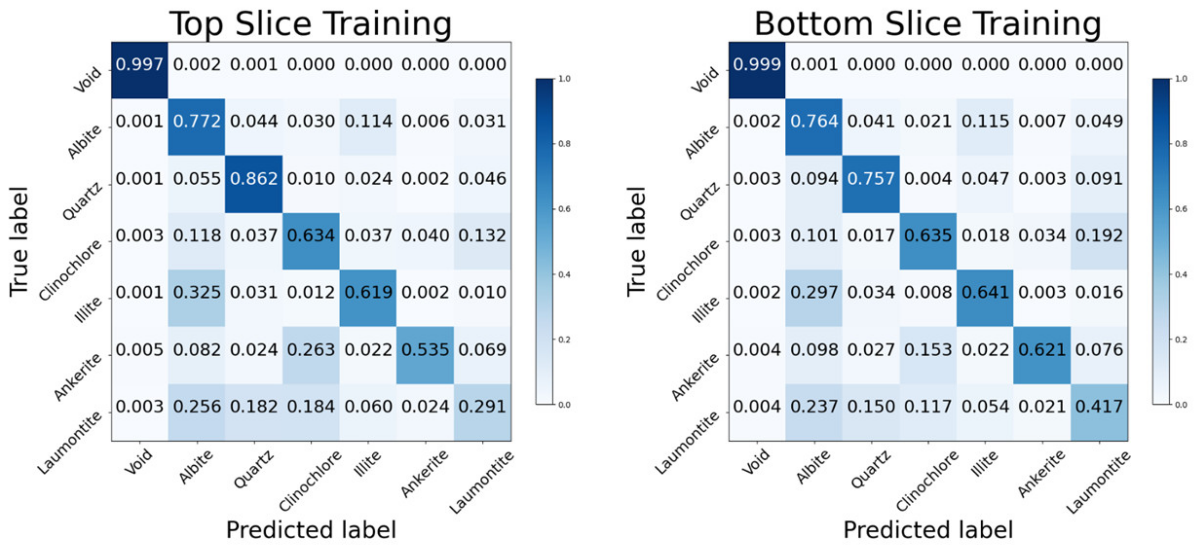
Further analysis of the pixel accuracy of the segmentation model is represented as a confusion matrix, as shown in Figure 7. The confusion matrix shows the proportion of predicted mineral pixel labels from the segmentation model for each mineral class with the true mineral pixel labels from the μXRF maps. This provides insights into the types of errors made by the model—in essence what predictions the model is confused by. For a model with high accuracy, the confusion matrix would possess high accuracies along the diagonal, from top left to bottom right. The overall profile of the confusion matrix between the two surfaces measured was similar, with similar pixel accuracies across all mineral phases. This indicates the consistency of the segmentation performance on different surfaces.
The accuracy of the void phase occurring mainly outside of the sample was correctly identified and, hence, the model was able to discern sample from empty space. Meanwhile, the mineral phases within the material varied in accuracy. The two predominant minerals consisted of albite and illite, as shown in Figure 6. The model was able to discern the difference between the two primary mineral phases, even though the phases were visually difficult to distinguish due to the similar greyscale intensities. Additionally, the model was able to overcome the intensity gradient from beam hardening to match the general segmentation from the training data. However, as can be seen in the confusion matrices for both surfaces in Figure 7, the majority of the incorrect labels for each of the two phases were attributed to the other phase. This suggests the task is inherently challenging and the model cannot separate the albite and illite confidently.
Among the discrete grains of minerals in the sample, the quartz phase is identified with the highest accuracy. Many of its false labels were from the surrounding minerals of albite and illite; the other major contributor was laumontite, which typically occurs in and around the quartz grains, and this is to be expected. Laumontite was the least accurate phase with less than half of the pixels labelled correctly for both surfaces, where the low quality of segmentation was also apparent from visual inspection. This was because the occurrence of laumontite is often in intricate fine structures, which requires highly accurate registered μXRF data to provide the model with strongly relevant training data. This has resulted in mislabelling with mostly albite, quartz and clinochlore. For clinochlore, 63% of the pixels were labelled correctly and mislabelled pixels were mainly laumontite and albite. Finally, ankerite had an average of 58% of pixels correctly identified with the largest proportion of mislabelling occurring with clinochlore. This was because both ankerite and clinochlore are relatively dense, causing a similar greyscale tomography intensity. The accuracy was further compounded by the relatively small abundance of ankerite, whereby any mislabelling would constitute a large percentage of labels.

3.2.2. Validation Data

While the model performed well on segmenting the training data, the true test for generalisability is to validate how well the model performs for data it has not been exposed to at all. In this case, this would be additional labelled slices within the sample. For this purpose, a thin slice (ca. 2 mm) of the plug was removed from the bottom and top part of the sample to expose such surfaces to generate validation data.
Figure 8b,h show the mineral labels for the top and bottom surfaces from within the bulk of the sample. The same mineral identification approach was performed as with the training dataset using K-means clustering analysis of the μXRF maps. Figure 8c,i show the segmentation results from the model that was trained from the outer slices. From visual inspection, the segmentation model performed well in extracting the defined course-grained minerals. In comparison to the training data, the model was able to recognise the approximate distribution of the matrix minerals of albite and illite, though not to the same accurate degree as the training data in Figure 6. In general, the performance on the validation data was lower than the training data as shown by accuracies of 63.50% and 62.79% from the top and bottom surfaces with the voids excluded, respectively.
Figure 9 shows the confusion matrix for the validation data. As with the training surfaces, the profile of the confusion matrix was similar with the validation surfaces, with a comparable spread of correct and incorrect label accuracies. Based on the two predominant minerals of albite and illite, there was an overprediction of the albite labels and underprediction of the illite labels. Quartz, conversely, was predicted well by the model with over 82–84% of the phase being predicted correctly. Clinochlore had an accuracy of 56–61% for both slices. Similar to the segmentation of the training data, the mislabels were mainly attributed to laumontite and, to a lesser extent, albite. Meanwhile, laumontite reached an accuracy of 26–28% for both slices. The mislabels occurred significantly across all other mineral phase labels. As previously suggested, this may be caused by a combination of the inappropriately minimal registration of the indistinct structure and the ambiguous greyscale intensity in the µCT dataset. Finally, ankerite had different performances across the two slices. For the top slice, the accuracy reached 44%, while for the bottom slice it was 38%. The majority of the mislabels occur with clinochlore. This was due to the fact of having similar densities, which resulted in similar greyscale values in the µCT dataset.
Figure 10 shows the 3D volume rendering of the tomography collected from the basaltic andesite sample in addition to the deep learning segmentation that was trained on the top and bottom surfaces of the sample. In terms of segmentation quality, the coarse grains show clear inconsistencies in the segmentation of the 2D orthoslices, although the model can distinctly identify the position and shape of the grains. Moreover, the model was also able to generalise details regarding the coarse-grained mineral structures. For example, the higher density inclusions within and around quartz were specifically recognised as laumontite, while other similarly dense minerals were correctly identified as clinochlore. For the fine-grained minerals of albite and illite, the model showed the ability to separate these minerals, which have faint intensity differences that are difficult to separate from visual observation and conventional thresholding methods. With the perspective of the 3D volume rendering, it is also possible to see apparent striations of the minerals perpendicular to the long axis of the cylindrical sample. This is because the segmentation model was two-dimensional and was applied on each orthoslice. Hence, this shows a lack of connection in terms of contextual segmentation information between the orthoslices and limits the continuity along the long axis of the cylindrical sample.
The relative abundances of the minerals throughout the sample from the Deep-XFCT segmentation is shown in Table 4. The abundances are in good agreement with the results obtained from μXRF mineral analysis of the top and bottom surface of the sample, shown in Table 2 and Table 3 respectively. Evidently, albite comprises the majority of the sample at approximately half of the sample, followed by illite, quartz, laumontite, clincochlore and ankerite. However, these mineral abundances in comparison with XRD (Table 1) show some discrepancies, specifically showing an 8.71% lower illite and a 6.94% higher laumontite and clinochlore abundance. These discrepancies are within the margin of error when considering that the smaller volume sampled by XRD may not be representative of the whole core plug as can be seen by the mineral distribution heterogeneity. Given that XRD is an important tool for validating mineral phases, it is important to try and ensure the sampling is representative of the entire core by ensuring that the largest possible volume of powder is used.

4. Discussion

In comparison to existing techniques that probe similar mineral domains, Deep-XFCT introduces a novel approach that exploits the benefits of artificial intelligence. Specifically, Deep-XFCT is able to extract a fully segmented 3D grain structure non-destructively and at large enough scales to accommodate a cylindrical core plug with measurements of approximately 24.3 mm in diameter and 25.9 mm in length. The results show Deep-XFCT works well in practice and should compare favourably to the conventional approaches of segmenting minerals, such as intensity thresholding, top-hat or watershed segmentation that can be affected by intensity inhomogeneity from beam hardening and experimental artefacts. In the context of its intended purpose for 3D mineral liberation analysis, Deep-XFCT can isolate grain locations and provide clear indications and realistic perspectives of the 3D morphology, distribution and abundance of minerals throughout the bulk volume of the core plug.
Furthermore, the use of deep learning extends the possible capabilities of segmentation through computer vision and removes the significant contribution of user bias to provide an objective approach with mineral segmentation. This is exemplified with the model to not only identify the coarse grains, but to also to discern minerals of similar greyscale intensities between the fine-grained minerals of albite and illite. Such a result would be valuable for mineral liberation analysis and unattainable through conventional methods. It could be argued that the distribution of albite and illite are similar throughout the length of the core plug sample, and therefore the model generalised the distribution. However, the model works in smaller isolated patches of each orthoslice, which would mean the model can recognise the imperceptible differences in intensity to assign either albite or illite. Furthermore, Deep-XFCT possesses advantages of minimal sample preparation and uses relatively accessible instrumentation and software to provide an approachable and practical method of 3D mineral liberation analysis.

4.1. Contributing Factors to Results

In comparison to existing methods that provide similar mineral information, such as QEMSCAN and FIB-SEM tomography, Deep-XFCT extends past surface information into large volumes and in a non-destructive manner. However, the two surface techniques have several advantages over the Deep-XFCT approach. QEMSCAN and FIB-SEM tomography can extract mineral information at higher resolutions due to the inherent properties of electrons in comparison to X-rays, although this can result in sampling bias if only small areas of the sample are imaged. Further, with Deep-XFCT, there is more manual handling of the data at this point of development in contrast to the QEMSCAN and FIB-SEM tomography. Moreover, there are several universal factors that can contribute to the inaccurate mislabelling of minerals for the basaltic andesite sample that limit the performance of the current implementation of Deep-XFCT. Though at the core of the problem all such issues stem from the mismatch of the μXRF and μCT data to produce accurate training data with correct pixel labels for the deep learning model, which will be discussed in the following.
Firstly, the K-means clustering approach has direct effects on the quality of the training and validation data. While the number of clusters was determined by the number of minerals obtained from XRD mineral analysis, the K-means approach is also dependent on the initial values. This effect was dealt with by randomising the initial values across 10 runs and using the best output in terms of inertia. Additionally, outliers can affect the results, and this was mitigated by masking the μXRF maps with the corresponding μCT surface to ensure only relevant pixels associated with the surface were included in the clustering. However, unbalanced data, in addition to outliers, can affect results and need to be considered. While not required with this current work as the K-means provided a sufficient result, other clustering algorithms can be used that account for unbalanced data and outliers, such as DBSCAN or OPTICS [42,43].
Secondly, the registration between the μXRF and μCT data is not perfectly aligned, as there is not a perfect correspondence between the grain shapes between the two datasets (Figure 5). Therefore, at a per-pixel scale, the information from μCT likely does not correlate completely with the mineral phase identification, leading to unambiguously incorrect labels for the μCT data. Further, defining the interfaces between grains is important for the network to recognise the features. This issue is exemplified by laumontite, as it commonly appears in fine intricate structures in and around quartz and has shown to be difficult to register perfectly. The addition of an added degree of freedom from the 2D orthoslice to the 3D tomogram also introduces imperfections in the registration. However, at the larger scale of the coarse mineral grains, the imperfect registration does not affect the overall performance as there is a representative quantity of correct labels to overcome the incorrect labels.
Thirdly, the resolution of both the μXRF and μCT measurements limits the accuracy of the resulting segmentation model. This was the case with the μXRF data, where the pixel resolution was 40 µm as opposed to the approximately 10 µm from the μCT data. The up-sampling of the μXRF pixels into the higher resolution geometry of the μCT pixels would lead to incorrect labelling of the μCT pixels, which would cause the model to have invariably incorrectly labelled training data. Therefore, the limiting resolution of the μXRF data also prohibits the method from being implemented on fine-grained minerals for the time being and restricted to coarse-grained minerals. However, based on the μXRF instrumentation, the resolution can be improved to 10 microns on smaller areas with the drawback of reducing the quantity of training data.
The issues mentioned relating to mismatching datasets are unavoidable when using inherently different techniques and must be viewed in their usefulness for the desired applications. A possible approach to resolve many of the issues would be to introduce an intermediary step within the segmentation workflow. This would involve first training a traditional machine learning model with a sparse dataset that does not require all pixels in the training data to be labelled. The training data could be produced through an erosion process of the defined grains from the μXRF analysis. This machine learning model would recognise minerals by their greyscale intensity in the μCT data and provide a segmentation that would define the interfaces better than the raw μXRF input. As a result, this segmentation from a traditional machine learning model could be more appropriate as a dense training set with all pixels labelled for training the deep learning model.
In terms of discussing the aspects of the deep learning process, an obvious concern is whether the quantity of training data is adequate, as having more training data is usually desirable. The training data sourced from the top and bottom of the sample appears to be sufficient for training the model to recognise the features required for mineral liberation analysis. This is contingent on the training data having satisfactory representation of all minerals, interfaces, shapes and features that would be present throughout the sample. The quality of such mineral maps could be improved through higher-resolution scans with other electron-based microscopy for both training and validation purposes. The quantity of training data could be increased by cutting the cylindrical core plug into a prism with additional flat surfaces suitable for μXRF analysis. Another concern relates to the relatively large patch size of 128 × 128 pixels that may have affected results; where the larger the patch size, the greater loss in detecting smaller details [44]. Conversely, a smaller patch size would not be able to access the larger features of minerals outside of each patch, limiting its usefulness. Therefore, the patch size selected for the deep learning model, whilst not able to discern the finer mineralogical details, was the best compromise in balancing segmented details at different scales.
Considering the possible limitations and shortcomings of the Deep-XFCT technique, and when comparing to conventional segmentation methods, the overarching goal to extract mineral attributes in a semi-automated fashion for the purposes of mineral liberation analysis was successfully performed for this specific collection of minerals.

4.2. Segmentation Enhancement Pathways

While the Deep-XFCT approach performs well, there are multiple pathways of improvement that can be implemented. All improvements should focus on the main objective of obtaining the most accurate segmentation possible. To this end, the improvements can be separated into those for preparing and obtaining the best training data and those related to training the model.
The most simple and obvious improvement for the training data is increasing the quantity of training data. This can be achieved by increasing flat surfaces on the sample by trimming off sections, for example into a prism shape, to obtain more μXRF data. However, this may not be practical or preferable as the sample may need to be kept intact and more time is required to collect additional μXRF data. Similarly, the quality of the training is also important, and this can be facilitated through higher resolutions datasets from both μCT and μXRF by reducing the overall sample size to provide more detailed and accurate training data. Furthermore, to increase the statistical robustness of the clustering method on the μXRF maps, a high-resolution photo can be taken to be added as part of the K-means clustering dataset to provide another dimension of information in the form of visible light information. Finally, while the finer registration is automated, the coarse registration of finding the corresponding orthoslice within the 3D tomography data is manually intensive and tedious. The coarse registration can also be optimised through artificial intelligence, allowing the whole Deep-XFCT procedure to be streamlined through automation [45].
For the process of training the segmentation model, a possible enhancement to the original U-net model is to use a multiscale U-net model instead [46]. The architecture of the multi-scale patch-based model would use multiple patch sizes to capture different contextual information at various dimension scales. This is conducted by creating a model input image by separating the initial image into overlapping patches, followed by combining with smaller up-sampled patches and larger down-sampled patches. This would accommodate different dimension scales that will allow the elucidation of all mineral mineralogy within the sample. Additionally, the use of a 3D U-net model [47] would be able to remove the striation artifacts seen in the resulting segmentation when using a 2D model. However, the need for 3D training data for a 3D segmentation model would be difficult to manifest from μXRF maps collected from surfaces. Further, there is a significant increase in the computational cost to using a 3D segmentation model over a 2D model and must be considered based on the results required.

5. Conclusions

Deep-XFCT uses deep learning as the correlative bridge between the different modalities and dimensions of μXRF and μCT. A deep learning segmentation model was trained with the minerals identified on the top and bottom surfaces of a cylindrical core plug and segmentation results were validated with surfaces from within the original core plug. While Deep-XFCT did not provide pixel-level accurate segmentations, it demonstrated the ability to provide an excellent proxy for the purposes of obtaining the presence, location, distribution and morphology of grains dispersed throughout a core plug. Furthermore, this artificial intelligence augmented workflow was shown to segment fine-grained minerals of similar density that would be impossible by manual segmentation. Moreover, it is also a conceptually simple workflow that uses experimental instrumentation that is readily accessible at research and commercial institutions. It also possesses all the advantages of minimal sample preparation, analysis of large samples of full core plugs and uses non-destructive analysis techniques. Hence, Deep-XFCT is a viable and valuable technique that has the potential to expedite 3D mineral liberation analysis.
While the technique was demonstrated and optimised on a geological core plug example for mineral liberation applications, the fundamental workflow of combining unique information from the surface and propagating through a volume via deep learning algorithms can be adopted by a plethora of image-based techniques. With such vast directions in which the technique can grow and be applied, the current approach is foreseen to be a pivotal steppingstone in incorporating various modalities of analysis into comprehensible and enriched findings through artificial intelligence.

Supplementary Materials

The following supporting information can be downloaded at: https://www.mdpi.com/article/10.3390/en15155326/s1.

Author Contributions

Conceptualisation, P.K.M.T., C.M. and K.R.-L.; Formal analysis, P.K.M.T.; Investigation A.Y.H., H.W. and A.R.; Methodology, P.K.M.T., C.M. and K.R.-L.; Software, P.K.M.T.; Supervision, C.M. and K.R.-L.; Writing—Original Draft, P.K.M.T. and K.R.-L. All authors have read and agreed to the published version of the manuscript.

Funding

K.R. was funded by the Australian Research Council ARC DP170104550, DP170104557, LP170100233 and LE200100209. P.K.M.T. was funded by UNSW RIS RG193860: “Multi-Instrument, Multi-Modal Co-Registration of Tomographic Images.”

Data Availability Statement

The raw and processed data required to reproduce these findings cannot be shared at this time due to the technical limitations. The raw and processed data can be obtained from the corresponding author upon reasonable request.

Acknowledgments

The authors would like to acknowledge Simone Zanoni from the Biological Resources Imaging Laboratory, UNSW Sydney, for providing background information on image analysis and registration. The authors acknowledge the use of the facilities at the Mark Wainwright Analytical Centre, UNSW Sydney, including the Spectroscopy Laboratory, X-ray Fluorescence Laboratory, X-ray Diffraction Laboratory and the Tyree X-ray CT Facility.

Conflicts of Interest

The authors declare no conflict of interest.

References

  1. Mariano, R.A.; Evans, C.L.; Manlapig, E. Definition of Random and Non-Random Breakage in Mineral Liberation—A review. Miner. Eng. 2016, 94, 51–60. [Google Scholar] [CrossRef]
  2. Lomberg, K. Best practice sampling methods, assay techniques, and quality control with reference to the platinum group elements (PGEs). J. S. Afr. Inst. Min. Metall. 2014, 114, 53–62. [Google Scholar]
  3. Sandmann, D. Use of Mineral Liberation Analysis (MLA) in the Characterization of Lithium-Bearing Micas. J. Miner. Mater. Charact. Eng. 2013, 1, 285–292. [Google Scholar] [CrossRef] [Green Version]
  4. Heinig, T.; Bachmann, K.; Tolosana-Delgado, R.; Boogaart, G.; Gutzmer, J. Monitoring gravitational and particle shape settling effects on MLA sampling preparation. In Proceedings of the IAMG, Freiberg, Germany, 5–13 September 2015. [Google Scholar]
  5. Tonžetić, Ž. 5—Quantitative analysis of iron ore using SEM-based technologies. In Iron Ore; Lu, L., Ed.; Woodhead Publishing: Sawston, UK, 2015; pp. 161–189. [Google Scholar] [CrossRef]
  6. Babel, B.; Penz, M.; Schach, E.; Boehme, S.; Rudolph, M. Reprocessing of a Southern Chilean Zn Tailing by Flotation—A Case Study. Minerals 2018, 8, 295. [Google Scholar] [CrossRef] [Green Version]
  7. Schulz, B. Editorial for Special Issue “Applications of SEM Automated Mineralogy: From Ore Deposits over Processing to Secondary Resource Characterization”. Minerals 2020, 10, 1103. [Google Scholar] [CrossRef]
  8. Sylvester, P.J. Use of the mineral liberation analyzer (MLA) for mineralogical studies of sediments and sedimentary rocks. Mineral. Assoc. Can. 2012, 1, 1–16. [Google Scholar] [CrossRef]
  9. Butcher, A.; Botha, P.W.; Dunks, C. An enabling geoscience tool for automated rock typing, stratigraphic refinement, and reservoir characterisation. APPEA J. 2008, 48, 482. [Google Scholar] [CrossRef]
  10. Goodall, W.R.; Scales, P.J.; Butcher, A.R. The use of QEMSCAN and Diagnostic Leaching in the Characterisation of Visible Gold in Complex Ores. Miner. Eng. 2005, 18, 877–886. [Google Scholar] [CrossRef]
  11. Gu, Y. Automated Scanning Electron Microscope Based Mineral Liberation Analysis An Introduction to JKMRC/FEI Mineral Liberation Analyser. J. Miner. Mater. Charact. Eng. 2003, 2, 33–41. [Google Scholar] [CrossRef]
  12. Voytekhovsky, Y. Modal Analysis of Rocks and Ores in Thin Sections. In International Congress on Applied Mineralogy; Springer: Cham, Switzerland, 2019; pp. 162–166. [Google Scholar]
  13. Lemmens, H.J.; Butcher, A.R.; Botha, P.W.S.K.B. “FIB/SEM and SEM/EDX: A New Dawn for the SEM in the Core Lab?,” Petrophysics-SPWLA. J. Form. Eval. Reserv. Descr. 2011, 52, 452–456. [Google Scholar]
  14. Guntoro, P.I.; Ghorbani, Y.; Parian, M.; Butcher, A.R.; Kuva, J.; Rosenkranz, J. Development and experimental validation of a texture-based 3D liberation model. Miner. Eng. 2021, 164, 106828. [Google Scholar] [CrossRef]
  15. Mutina, A.; Bruyndonckx, P. Combined micro-X-ray tomography and micro-X-ray fluorescence study of reservoir rocks: Applicability to core analysis. Microsc. Anal. Anal. Suppl. 2013, 27, S4–S6. [Google Scholar]
  16. Vekemans, B.; Janssens, K.; Vincze, L.; Aerts, A.; Adams, F.; Hertogen, J. Automated segmentation of μ-XRF image sets. X-ray Spectrom. Int. J. 1997, 26, 333–346. [Google Scholar] [CrossRef]
  17. Arzilli, F.; Polacci, M.; Landi, P.; Giordano, D.; Baker, D.R.; Mancini, L. A novel protocol for resolving feldspar crystals in synchrotron X-ray microtomographic images of crystallized natural magmas and synthetic analogs. Am. Miner. 2016, 101, 2301–2311. [Google Scholar] [CrossRef] [Green Version]
  18. Juránek, R.; Výravský, J.; Kolář, M.; Motl, D.; Zemčík, P. Graph-based deep learning segmentation of EDS spectral images for automated mineral phase analysis. Comput. Geosci. 2022, 165, 105–109. [Google Scholar] [CrossRef]
  19. Song, Y.; Huang, Z.; Shen, C.; Shi, H.; Lange, D.A. Deep learning-based automated image segmentation for concrete petrographic analysis. Cem. Concr. Res. 2020, 135, 106118. [Google Scholar] [CrossRef]
  20. Tang, K.; Meyer, Q.; White, R.; Armstrong, R.T.; Mostaghimi, P.; Da Wang, Y.; Liu, S.; Zhao, C.; Regenauer-Lieb, K.; Tung, P.K.M. Deep learning for full-feature X-ray microcomputed tomography segmentation of proton electron membrane fuel cells. Comput. Chem. Eng. 2022, 161, 107768. [Google Scholar] [CrossRef]
  21. McCoy, J.; Auret, L. Machine learning applications in minerals processing: A review. Miner. Eng. 2018, 132, 95–109. [Google Scholar] [CrossRef]
  22. Bu, X.; Zhou, S.; Danstan, J.K.; Bilal, M.; Hassan, F.U.; Chao, N. Prediction of coal flotation performance using a modified deep neural network model including three input parameters from feed. Energy Sources Part A Recover. Util. Environ. Eff. 2022, 1–13. [Google Scholar] [CrossRef]
  23. Bu, X.; Vahed, A.T.; Ghassa, S.; Chelgani, S.C. Modelling of coal flotation responses based on operational conditions by random forest. Int. J. Oil Gas Coal Technol. 2021, 27, 457. [Google Scholar] [CrossRef]
  24. Chelgani, S.C.; Nasiri, H.; Alidokht, M. Interpretable modeling of metallurgical responses for an industrial coal column flotation circuit by XGBoost and SHAP-A “conscious-lab” development. Int. J. Min. Sci. Technol. 2021, 31, 1135–1144. [Google Scholar] [CrossRef]
  25. Tohry, A.; Yazdani, S.; Hadavandi, E.; Mahmudzadeh, E.; Chelgani, S.C. Advanced modeling of HPGR power consumption based on operational parameters by BNN: A “Conscious-Lab” development. Powder Technol. 2020, 381, 280–284. [Google Scholar] [CrossRef]
  26. Tohry, A.; Chelgani, S.C.; Matin, S.; Noormohammadi, M. Power-draw prediction by random forest based on operating parameters for an industrial ball mill. Adv. Powder Technol. 2020, 31, 967–972. [Google Scholar] [CrossRef]
  27. Sauter, E.; Sarikaya, E.; Winter, M.; Wegener, K. In-process detection of grinding burn using machine learning. Int. J. Adv. Manuf. Technol. 2021, 115, 2281–2297. [Google Scholar] [CrossRef]
  28. Ahmed, M.M. Effect of comminution on particle shape and surface roughness and their relation to flotation process. Int. J. Miner. Process. 2010, 94, 180–191. [Google Scholar] [CrossRef]
  29. Weber, C.R.; Vlahovic, W.; Wyborn, D. Validation of Hot Rock Geothermal Energy Resources; Milestone 2 Report to the Australian Greenhouse Office Under the Renewable Energy Commercialisation Program. R00032661 (GS2002/117); Geological Survey of New South Wales (DiGS): Hunter Valley, Australia, 2001.
  30. Philpotts, A.R.; Ague, J.J. Principles of Igneous and Metamorphic Petrology, 2nd ed.; Cambridge University Press: Cambridge, UK, 2010. [Google Scholar]
  31. Lafuente, B.; Downs, R.T.; Yang, H.; Stone, N. The power of databases: The RRUFF project. In Highlights in Mineralogical Crystallography; Walter de Gruyter GmbH: Berlin, Germany, 2016; pp. 1–29. [Google Scholar]
  32. Pedregosa, F.; Varoquaux, G.; Gramfort, A.; Michel, V.; Thirion, B.; Grisel, O.; Blondel, M.; Prettenhofer, P.; Ron Weiss, R.; Duchesnay, E.; et al. Scikit-learn: Machine learning in Python. J. Mach. Learn. Res. 2011, 2, 2825–2830. [Google Scholar]
  33. Dragonfly Software, 2021.2; Object Research Systems (ORS) Inc.: Montreal, QC, Canada, 2021.
  34. Tomasi, C.; Manduchi, R. Bilateral Filtering for Gray and Color Images. In Proceedings of the Sixth International Conference on Computer Vision (IEEE Cat. No. 98CH36271), Bombay, India, 7 January 1998; pp. 839–846. [Google Scholar]
  35. Maes, F.; Collignon, A.; Vandermeulen, D.; Marchal, G.; Suetens, P. Multimodality image registration by maximization of mutual information. IEEE Trans. Med. Imaging 1997, 16, 187–198. [Google Scholar] [CrossRef] [Green Version]
  36. Ronneberger, O.; Fischer, P.; Brox, T. U-net: Convolutional Networks for Biomedical Image Segmentation. In International Conference on Medical Image Computing and Computer-Assisted Intervention; Springer: Cham, Switzerland, 2015; pp. 234–241. [Google Scholar]
  37. Li, X.; Sun, X.; Meng, Y.; Liang, J.; Wu, F.; Li, J. Dice Loss for Data-imbalanced NLP Tasks. In Proceedings of the 58th Annual Meeting of the Association for Computational Linguistics, Online, 5–10 July 2020; Association for Computational Linguistics: Stroudsburg, PA, USA, 2020; pp. 465–476. [Google Scholar]
  38. Sudre, C.H.; Li, W.; Vercauteren, T.; Ourselin, S.; Cardoso, M.J. Generalised Dice Overlap as a Deep Learning Loss Function for Highly Unbalanced Segmentations. In Deep Learning in Medical Image Analysis and Multimodal Learning for Clinical Decision Support; Springer: Cham, Switzerland, 2017; pp. 240–248. [Google Scholar] [CrossRef] [Green Version]
  39. Crum, W.; Camara, O.; Hill, D. Generalized Overlap Measures for Evaluation and Validation in Medical Image Analysis. IEEE Trans. Med Imaging 2006, 25, 1451–1461. [Google Scholar] [CrossRef]
  40. Zeiler, M.D. Adadelta: An adaptive learning rate method. arXiv 2012, arXiv:12125701. [Google Scholar]
  41. Rietveld, H.M. The rietveld method. Phys. Scr. 2014, 89, 098002. [Google Scholar] [CrossRef]
  42. A Density-Based Algorithm for Discovering Clusters in Large Spatial Databases with Noise. In Proceedings of the Second International Conference on Knowledge Discovery and Data Mining, Portland, OR, USA, 2–4 August 1996; Available online: https://dl.acm.org/doi/10.5555/3001460.3001507 (accessed on 15 July 2022).
  43. Ankerst, M.; Breunig, M.M.; Kriegel, H.; Sander, J. OPTICS: Ordering Points to Identify the Clustering Structure. ACM Sigmod Record 1999, 28, 49–60. [Google Scholar] [CrossRef]
  44. Hamwood, J.; Alonso-Caneiro, D.; Read, S.A.; Vincent, S.; Collins, M.J. Effect of patch size and network architecture on a convolutional neural network approach for automatic segmentation of OCT retinal layers. Biomed. Opt. Express 2018, 9, 3049–3066. [Google Scholar] [CrossRef] [PubMed] [Green Version]
  45. Seifert, R.; Markert, S.M.; Britz, S.; Perschin, V.; Erbacher, C.; Stigloher, C.; Kollmannsberger, P. DeepCLEM: Automated registration for correlative light and electron microscopy using deep learning. F1000Research 2020, 9, 1275. [Google Scholar] [CrossRef]
  46. Li, J.; Sarma, K.V.; Chung-Ho, K.; Gertych, A.; Knudsen, B.S.; Arnold, C.W. A Multi-scale U-Net for Semantic Segmentation of Histological Images from Radical Prostatectomies. AMIA Annu. Symp. Proc. AMIA Symp. 2017, 2017, 1140–1148. [Google Scholar]
  47. Içek, Ö.; Abdulkadir, A.; Lienkamp, S.S.; Brox, T.; Ronneberger, O. 3D U-Net: Learning Dense Volumetric Segmentation from Sparse Annotation. In Medical Image Computing and Computer-Assisted Intervention—MICCAI 2016; Springer: Cham, Switzerland, 2016; pp. 424–432. [Google Scholar] [CrossRef] [Green Version]
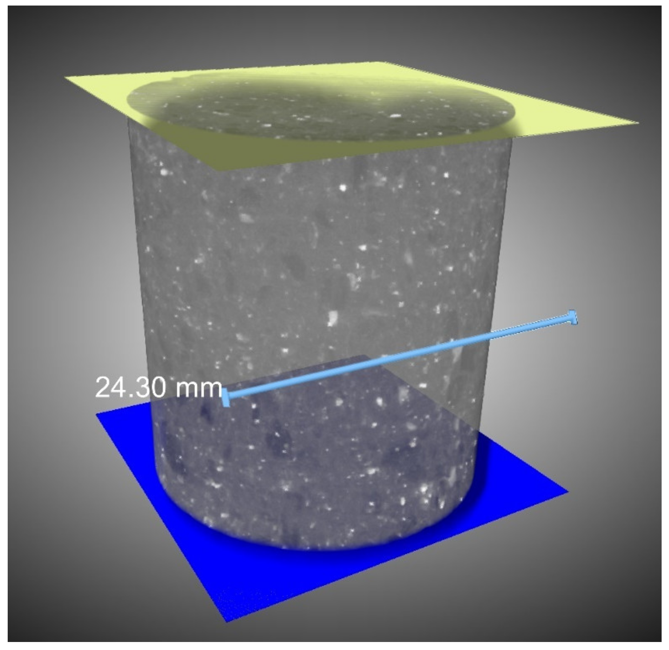
Figure 1. A μCT dataset of the basaltic andesite sample with the locations of the top and bottom surfaces scanned with μXRF in the yellow (top) and blue (bottom) planes.
Energies 15 05326 g001
Figure 2. Positions of point analysis (A–F) for μXRF and Raman measurements on the bottom surface of the core plug sample. These data were used in extension to the K-means clustering of the μXRF maps and XRD mineral analysis to elucidate mineral segmentation of the surface.
Energies 15 05326 g002
Figure 3. μXRF elemental maps from the bottom surface of the training data shown with greyscale intensities indicating elemental concentrations. The raw elemental maps show noisy artefacts on the lower right portion of the image from the long edge of the cylindrical drill core, as the flat faces of the sample were not parallel. This results in detection of X-ray signals from the long edge of the cylindrical sample. This artefact was removed by masking with the corresponding μCT image. The μXRF elemental maps from all surfaces collected can be found in the Supplementary Materials.
Energies 15 05326 g003
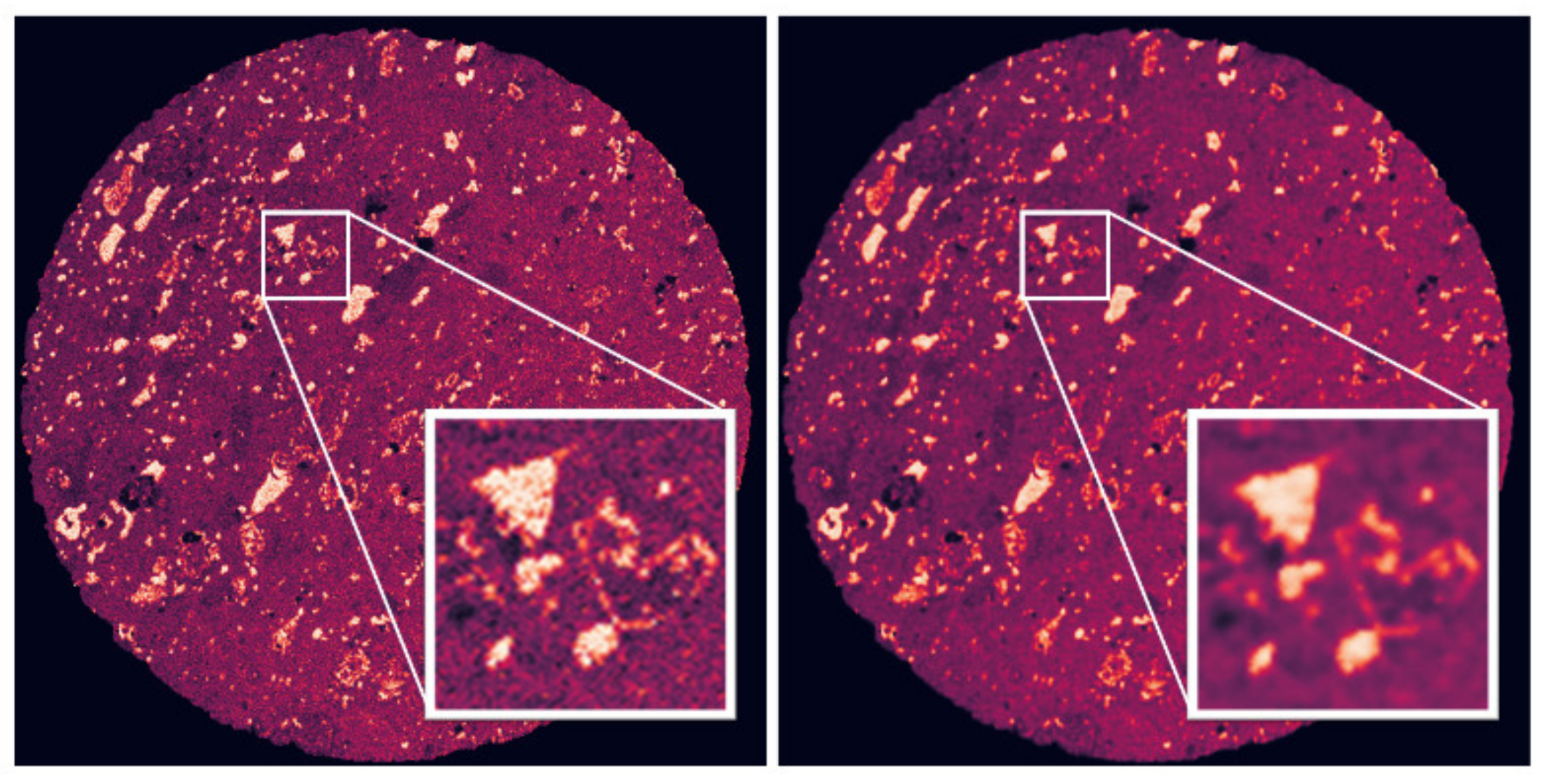
Figure 4. (Left) Raw μXRF map of Na, where the higher intensities indicate higher concentrations of Na. (Right) μXRF map of Na with bilateral filtering applied. The bilateral filtering reduces noise while preserving the edges, which is important in identifying homogenous grains and defining the interface between grains.
Energies 15 05326 g004
Figure 5. An opaque overlay of a Fe μXRF map (yellow) over the matching μCT orthoslice showing minor inaccuracies in the registration between the two datasets.
Energies 15 05326 g005
Figure 6. Training data from the top surface for (a) μCT data; (b) μXRF from K-means clustering; (c) deep learning segmentation; (df) zoomed areas as defined by the yellow inset box, respectively. The training data from the bottom surface is shown for (g) μCT data; (h) μXRF from K-means clustering; (i) deep learning segmentation; (jl) zoomed areas as defined by the blue inset box, respectively.
Energies 15 05326 g006
Figure 7. Pixel-wise confusion matrices for the segmentation of the top and bottom surfaces, showing the ratio of correctly and incorrectly predicted labels of the segmentation model in comparison to the true labels from the μXRF maps.
Energies 15 05326 g007
Figure 8. Validation data from the top surface for (a) μCT data; (b) μXRF from K-means clustering; (c) deep learning segmentation; (df) zoomed areas as defined by the yellow inset box, respectively. The validation data from bottom surface is shown for (g) μCT data; (h) μXRF from K-means clustering; (i) deep learning segmentation; (jl) zoomed areas as defined by the blue inset box, respectively.
Energies 15 05326 g008
Figure 9. Confusion matrices showing the predicted deep learning and true μXRF mineral pixel classifications for the validation data collected from the surfaces within the bulk of the basaltic andesite rock sample.
Energies 15 05326 g009
Figure 10. 3D tomography cutaway of the cylindrical basaltic andesite core plug (left) and the 3D segmentation performed by the deep learning model (right).
Energies 15 05326 g010
Table 1. XRD results of the mineral phases identified and their respective abundance percentages from a random selection of the sample.
Mineral IdentifiedChemical FormulaAbundance (%)
AlbiteAl1.488Ca0.491Na0.499O8Si2.50650.4 (±5.6)
Ankerite C2Ca0.997Fe0.676Mg0.273Mn0.054O61.4 (±0.1)
Clinochlore H16Al2.884Fe0.874Mg11.126O36Si5.1169.7 (±0.8)
Illite 2M C2Al4K1O12Si1212.0 (±1.5)
Laumontite H4Al2Ca1O14Si414.0 (±1.9)
Quartz SiO212.6 (±0.9)
Table 2. μXRF K-means clustering results. The clustering centroids for the μXRF maps of the bottom surface are shown as normalised 8 bit fluorescence intensities with a minimum of 0 and maximum of 255. Additionally, the abundance percentage of the labels are shown along with the assigned mineral.
Assigned MineralCentroid NumberColour on ImagesAl (Ct.)Ca (Ct.)Fe (Ct.)K (Ct.)Mg (Ct.)Mn (Ct.)Na (Ct.)Si (Ct.)µCT (Ct.)Abundance (%)
Albite1Red1491891105898613414815648
Ankerite2Grey4513412631659266532031.98
Clinochlore3Yellow72131912020322067731874.06
Illite4Light blue1631674167817513615915024.8
Laumontite5White12116118441311391131321557.06
Quartz6Dark blue182123627725218217912014
Table 3. Point analysis results from XRF and Raman: mass percent from the XRF and detection from Raman of the selected 20 µm spots in Figure 2. Note that for the XRF mass percentages, other trace elements detected were ignored, as they were not in the minerals detected by XRD. Additionally, it should be noted the mass percentages across the various minerals showed elements not found in their respective minerals, as the X-ray spot size also exposed the matrix minerals of albite and illite.
Assigned MineralLabel in Figure 2Raman DetectionAl Mass %Ca Mass %Fe Mass %K Mass %Mg Mass %Mn Mass %Na Mass %Si Mass %
AlbiteFDetected16.602.6111.934.881.660.248.8251.82
AnkeriteAUndetected16.123.2318.393.574.690.566.3345.54
ClinochloreCDetected15.883.1313.234.942.590.337.2451.10
IlliteDUndetected16.593.1410.306.771.090.237.6152.74
LaumontiteEUndetected16.293.2810.336.411.420.227.7052.73
QuartzBDetected16.352.038.722.371.960.248.7958.64
Table 4. Abundance percentage of each mineral obtained from segmentation with the deep learning model.
MineralDeep-XFCT Segmentation Abundance (%)
Albite50.48
Ankerite1.85
Clinochlore5.18
Illite20.71
Laumontite7.06
Quartz14.71
Publisher’s Note: MDPI stays neutral with regard to jurisdictional claims in published maps and institutional affiliations.