
Effect of Blade Diameter on the Performance of Horizontal-Axis Ocean Current Turbine


 , , ,
, , ,  and
and
Abstract
:1. Introduction
2. Theory
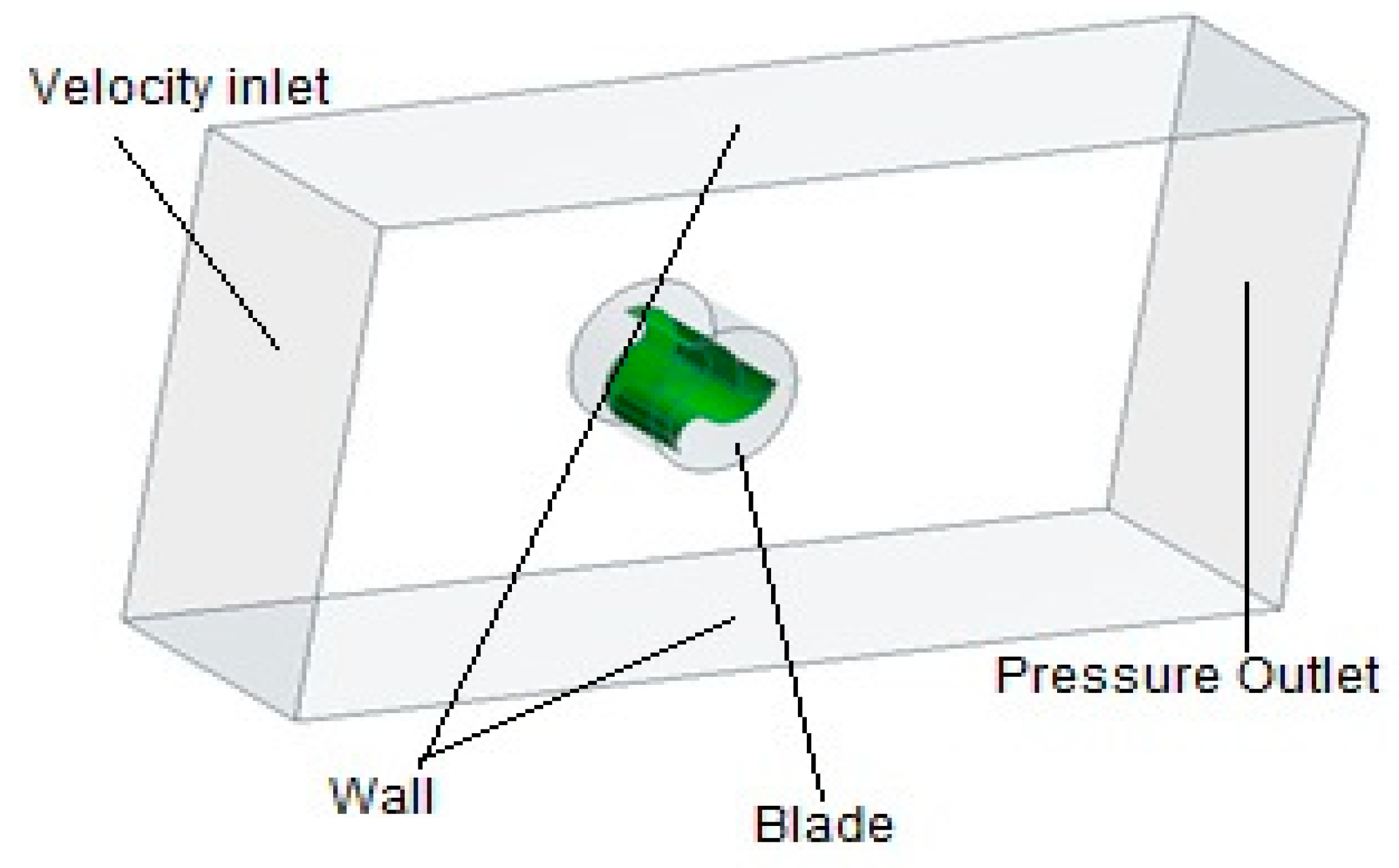
2.1. CFD Description
2.2. Standard k-ε Turbulence Model
2.3. Performance of Equation
3. Numerical Setup
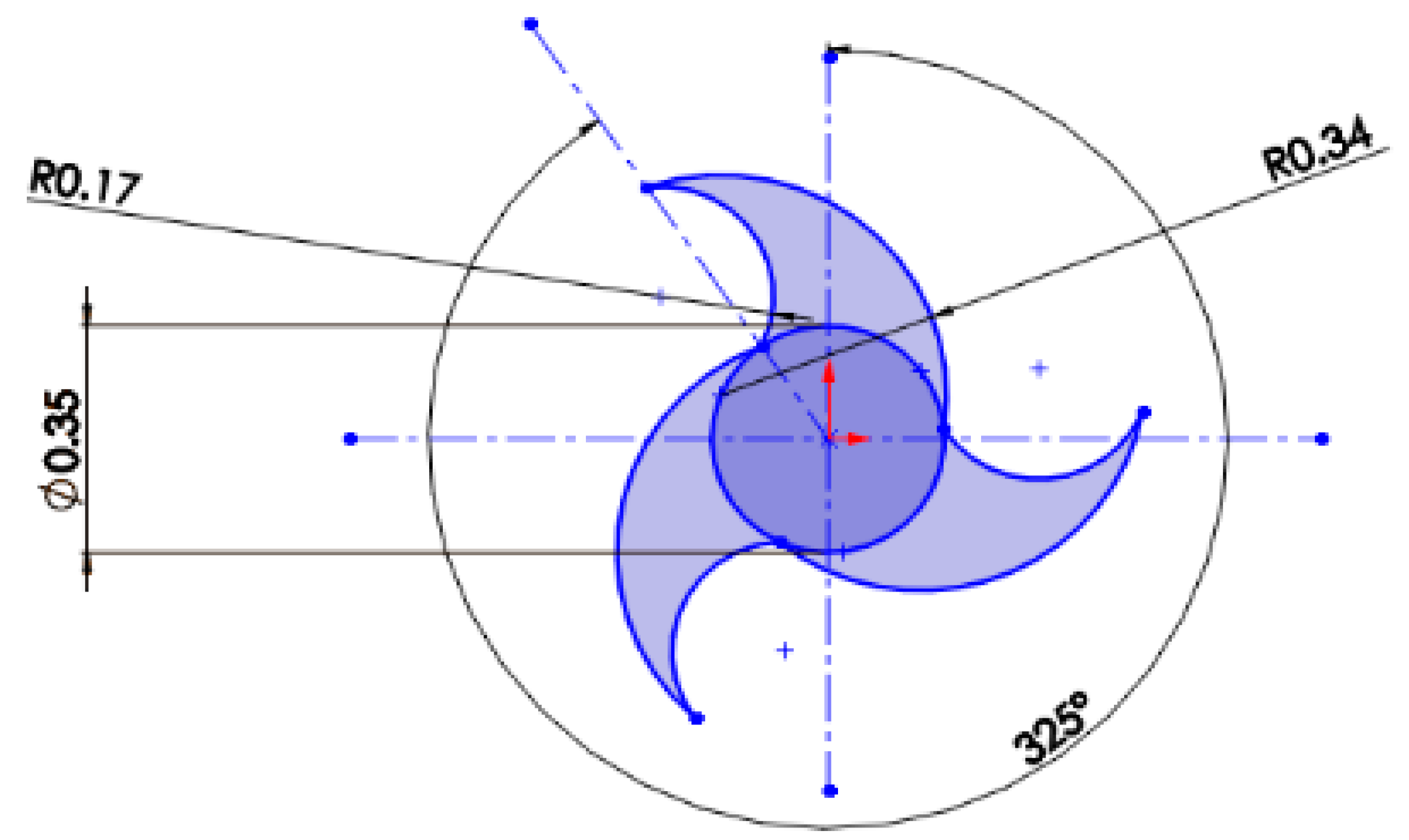
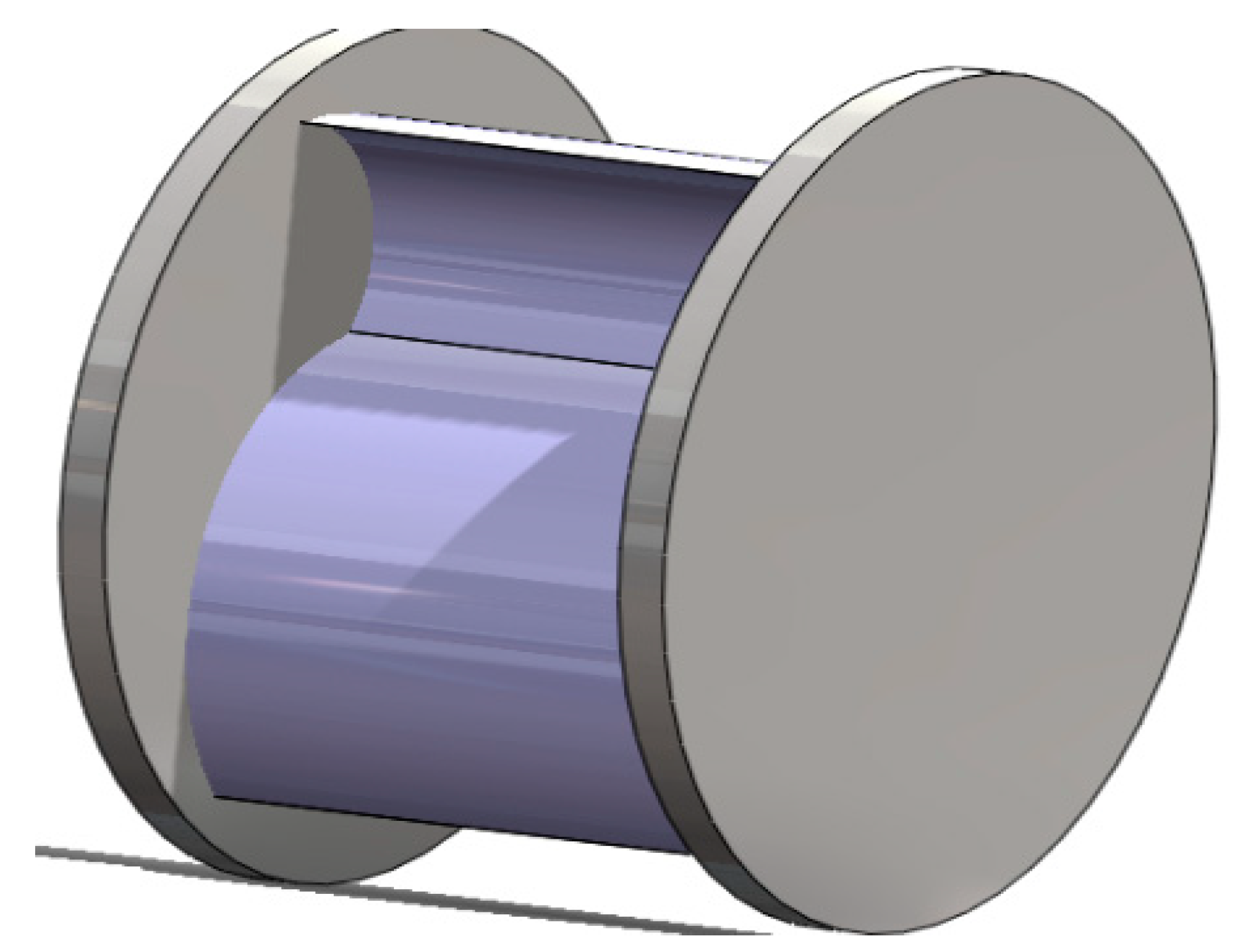
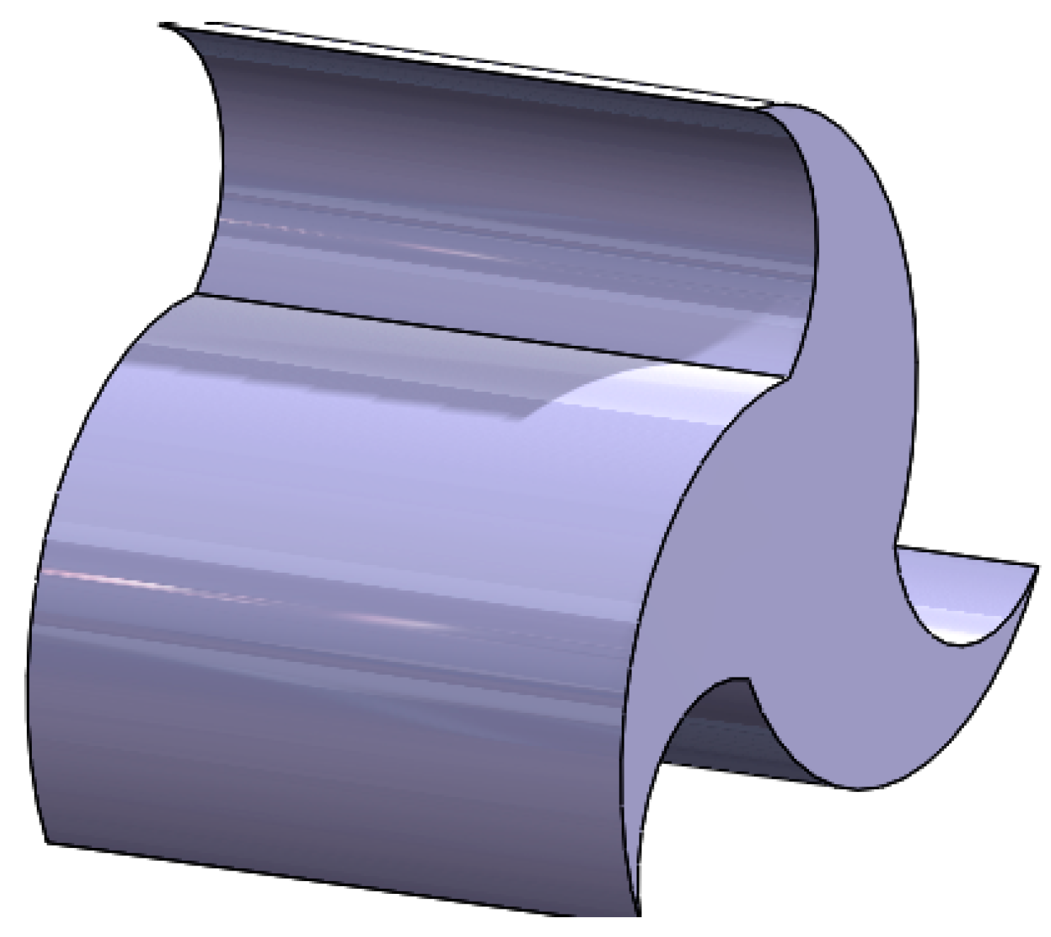
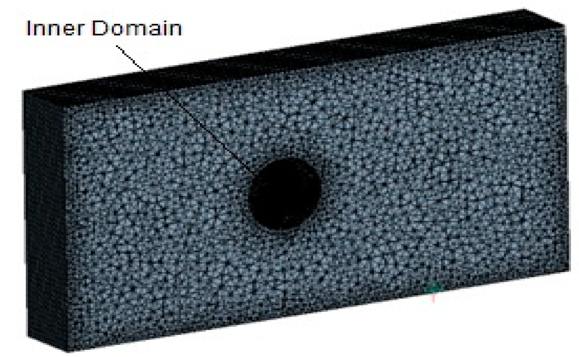
3.1. Geometry Modeling
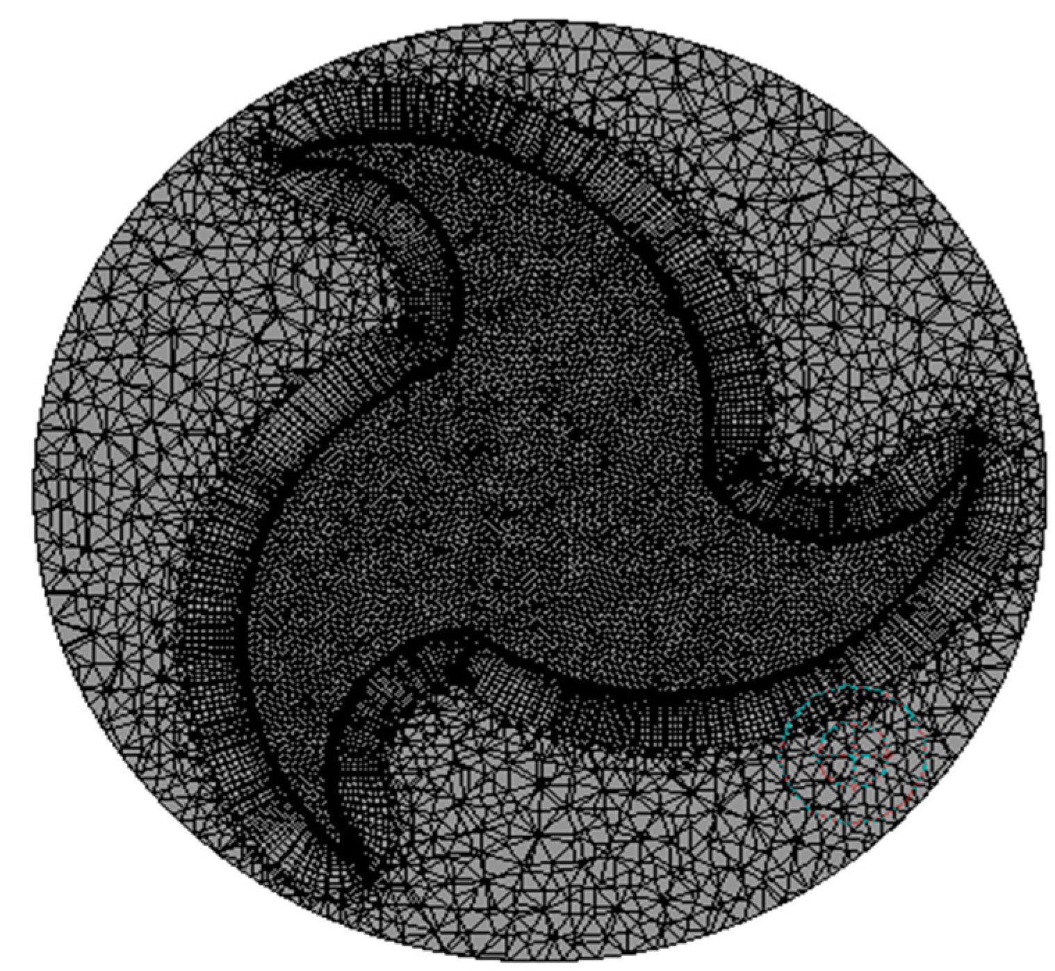
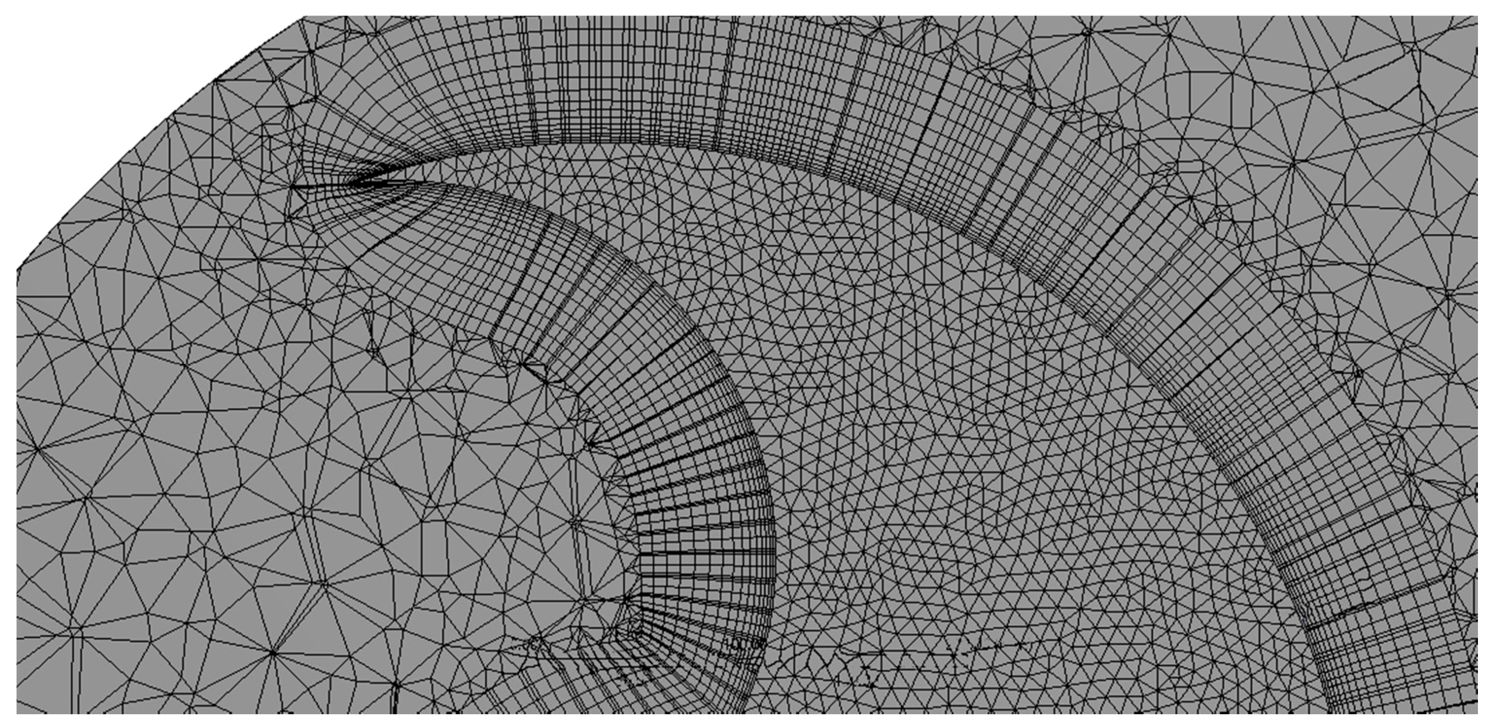
3.2. Meshing
4. Result and Discussion
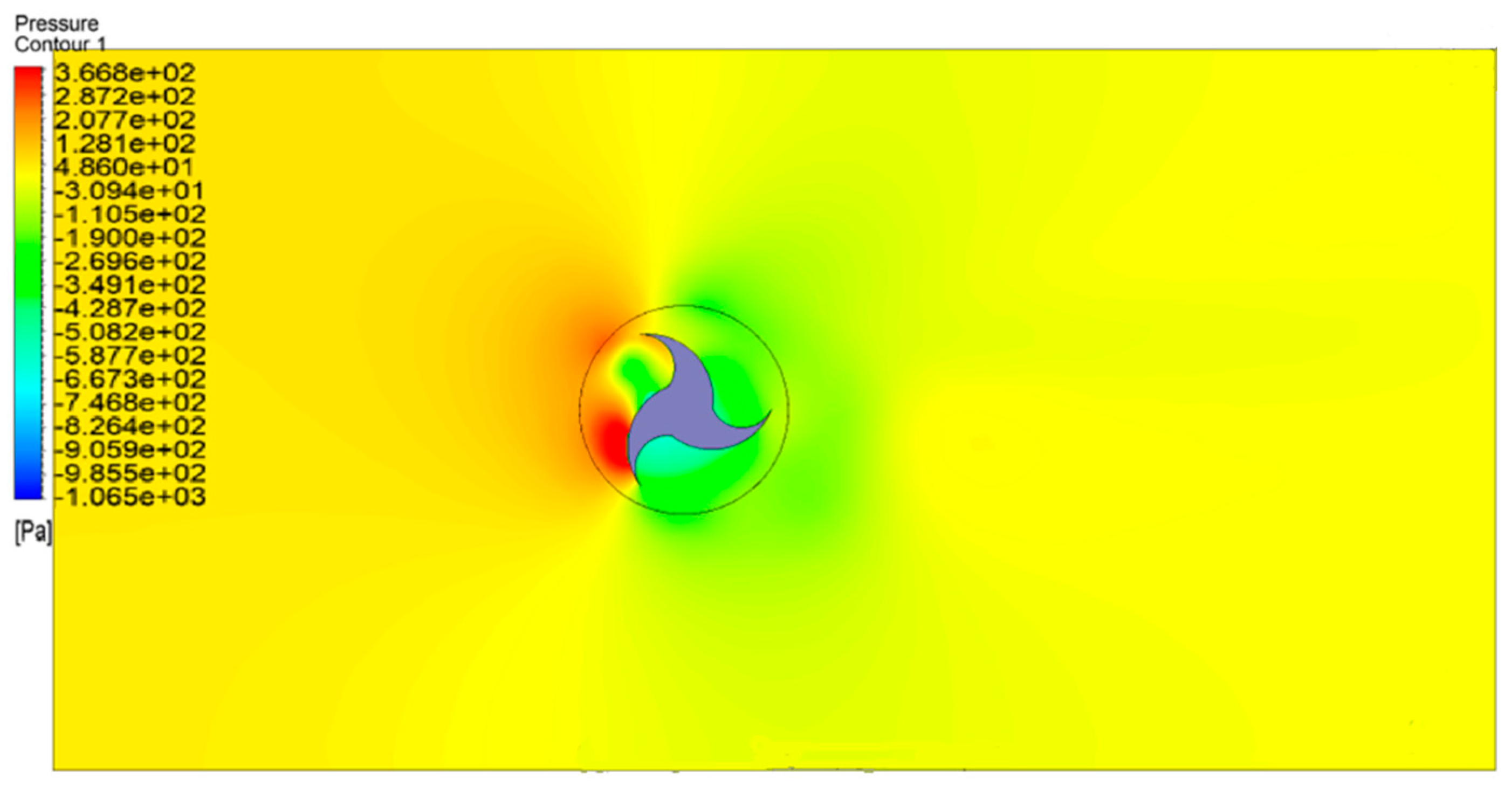
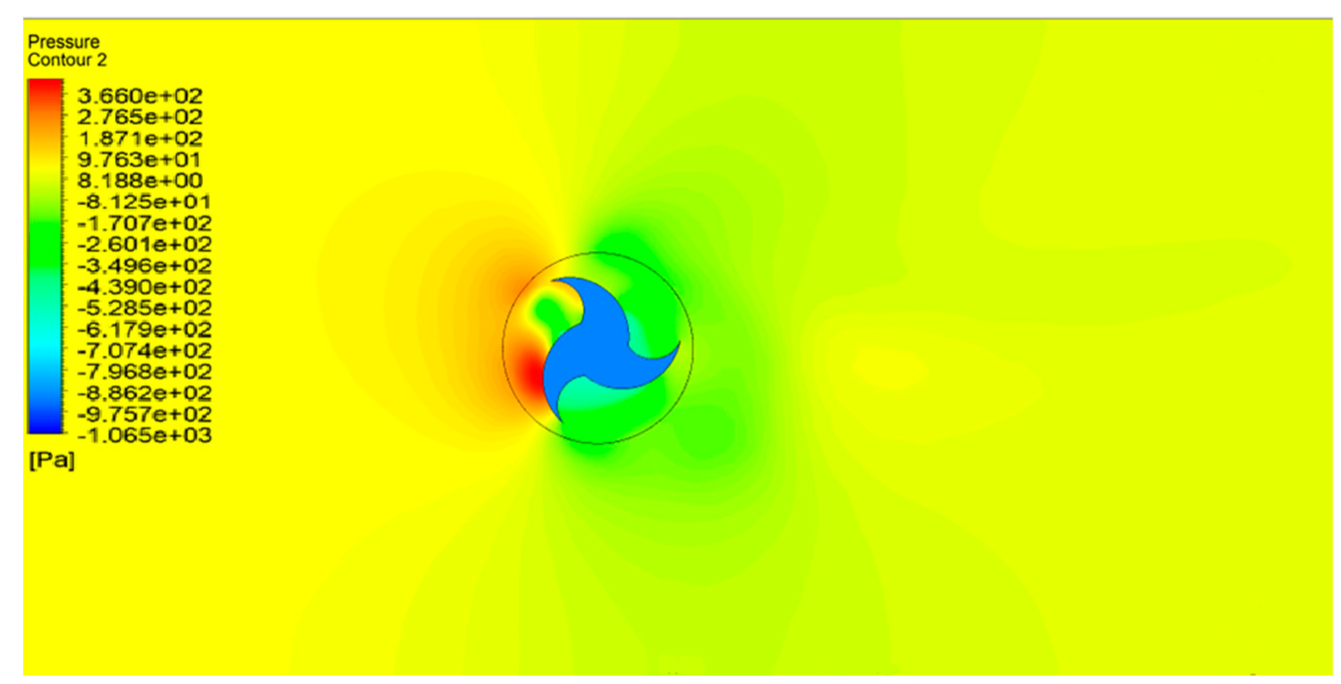
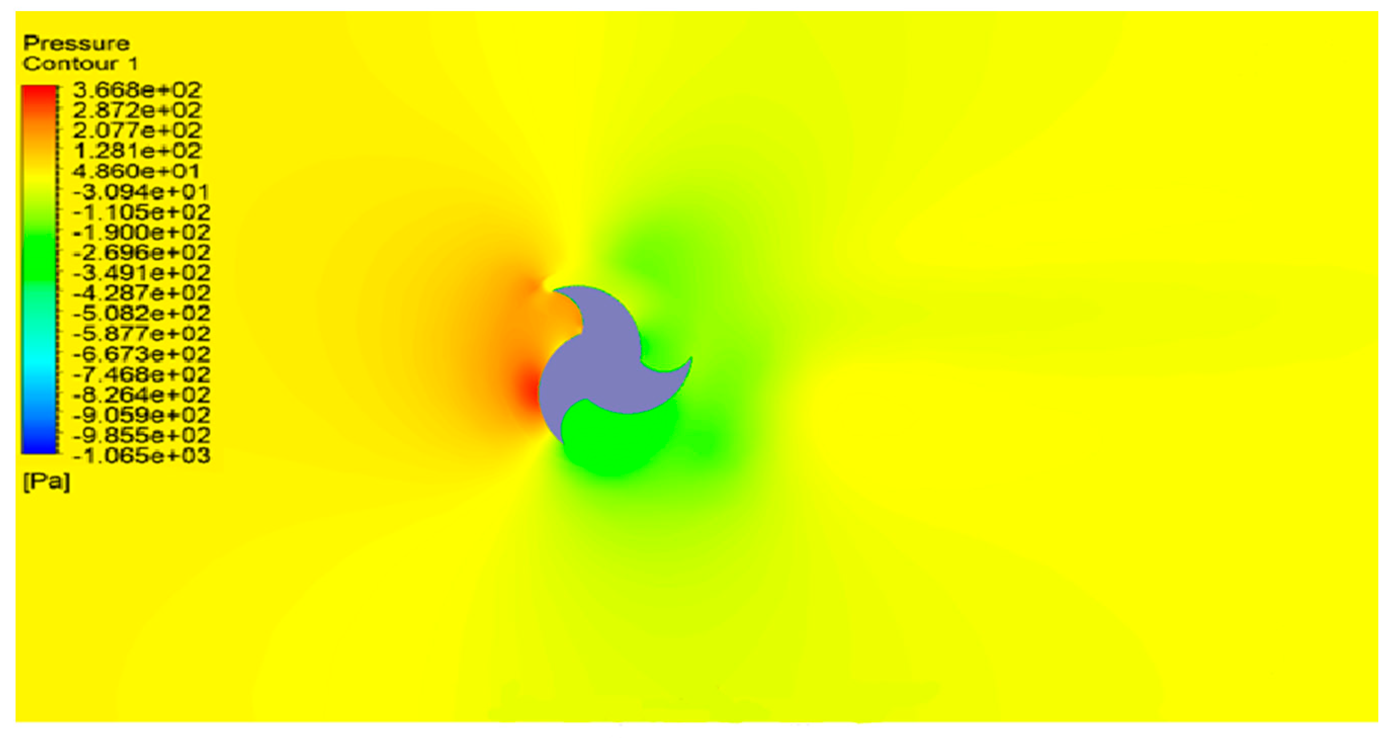
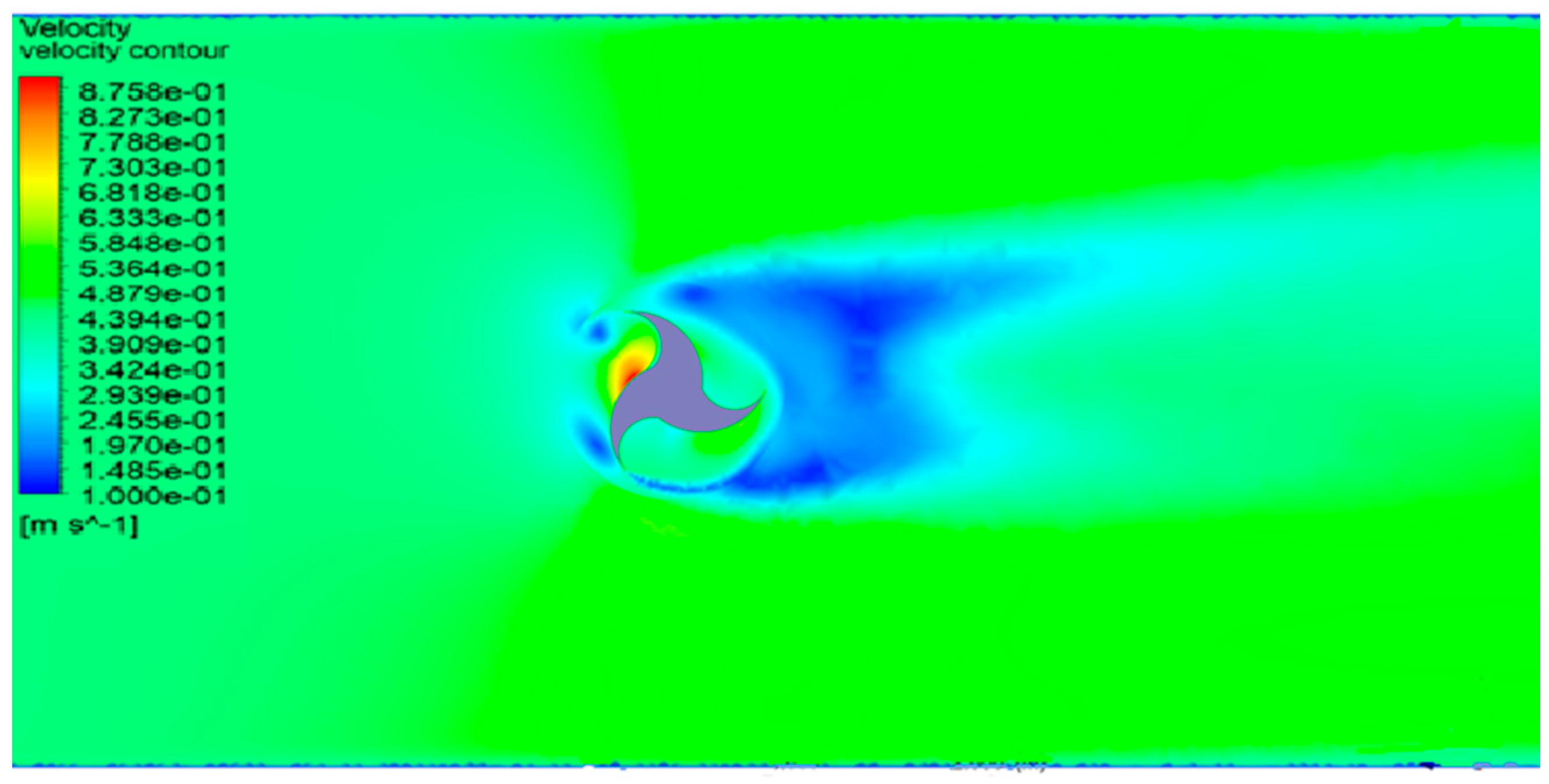
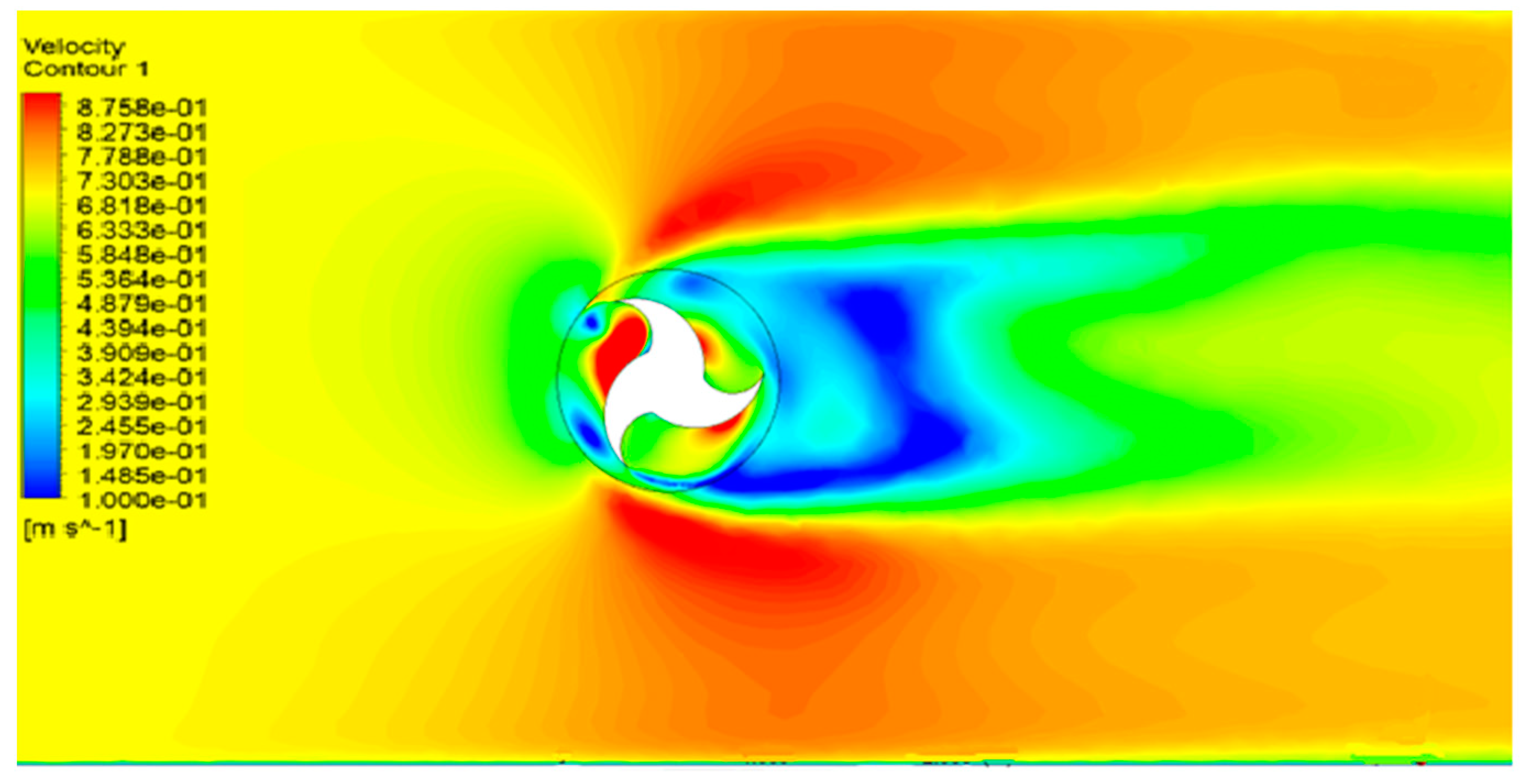
4.1. Velocity and Pressure Contour
4.2. Comparison of Torque and Power Curve
5. Conclusions
Author Contributions
Funding
Acknowledgments
Conflicts of Interest
Abbreviations and Symbols
| CFD | Computational Fluid Dynamics |
| HAOCT | Horizontal-Axis Ocean Current Turbine |
| VAOCT | Vertical-Axis Ocean Current Turbine |
| OCT | Ocean Current Turbine |
| TSR | Tip Speed Ratio |
| Nk | Production term of turbulent kinetic energy because of the gradient of mean velocity |
| Nb | The turbulent kinetic energy due to buoyancy |
| DM | Contribution of fluctuating dilation to the all-inclusive dissipation rate |
| xi | Coordinate in the ith direction |
| Dynamic viscosity | |
| Turbulent dynamic viscosity | |
| , | Turbulent Prandtl numbers for ‘k’ and ‘’ respectively, have a value of 0.39. |
| Ax, Ay, Az | Areas in the direction x, y, z, respectively |
| u, v, w | Velocities in the x, y, z-direction, respectively |
| A1ε, A2ε, A3ε | Model constants |
References
- Wellmann, J.; Morosuk, T. Renewable Energy Supply and Demand for the City of El Gouna, Egypt. Sustainability 2016, 8, 314. [Google Scholar] [CrossRef] [Green Version]
- Flavio, R.; Arroyo, M.; Miguel, L. The Trends of the Energy Intensity and CO2 Emissions Related to Final Energy Consumption in Ecuador: Scenarios of National and Worldwide Strategies. Sustainability 2020, 12, 20. [Google Scholar]
- Saba, A.M.; Khan, A.H.; Akhtar, M.N.; Khan, N.A.; Koloor, S.S.R.; Petrů, M.; Radwan, N. Strength and flexural behavior of steel fiber and silica fume incorporated self-compacting concrete. J. Mater. Res. Technol. 2021, 12, 1380–1390. [Google Scholar] [CrossRef]
- Bédard, R.; Jacobson, P.; Previsic, M.; Musial, W.; Varley, R. An Overview of Ocean Renewable Energy Technologies. Oceanography 2010, 23, 22–31. [Google Scholar] [CrossRef]
- Alipour, R.; Alipour, R.; Koloor, S.S.R.; Petrů, M.; Ghazanfari, S.A. On the Performance of Small-Scale Horizontal Axis Tidal Current Turbines. Part 1: One Single Turbine. Sustainability 2020, 12, 5985. [Google Scholar] [CrossRef]
- Nachtane, T.; Moumen, S. Design and Hydrodynamic Performance of a Horizontal Axis Hydrokinetic Turbine. Int. J. Automot. Mech. Eng. 2019, 16, 6453–6469. [Google Scholar] [CrossRef]
- Lestari, H.; Arentsen, M.; Bressers, H.; Gunawan, B.; Iskandar, J. Parikesit Sustainability of Renewable Off-Grid Technology for Rural Electrification: A Comparative Study Using the IAD Framework. Sustainability 2018, 10, 4512. [Google Scholar] [CrossRef] [Green Version]
- Magagna, D.; Uihlein, A. Ocean energy development in Europe: Current status and future perspectives. Int. J. Mar. Energy 2015, 11, 84–104. [Google Scholar] [CrossRef]
- Alipour, R.; Alipout, R.; Fardian, F.; Kollor, S.; Petru, M. Performance improvement of a new proposed Savonius hydrokinetic turbine: A numerical investigation. Energy Rep. 2020, 6, 3051–3066. [Google Scholar] [CrossRef]
- Le Traon, P.; Morrow, R. Ocean currents and eddies. In International Geophysics; Elsevier: Amsterdam, The Netherlands, 2001; pp. 171–215. [Google Scholar]
- Hu, S.; Sprintall, J.; Guan, C.; McPhaden, M.; Wang, F.; Hu, D.; Cai, W. Deep-reaching acceleration of global mean ocean circulation over the past two decades. Sci. Adv. 2020, 6, eaax7727. [Google Scholar] [CrossRef] [Green Version]
- Farokhi Nejad, A.; Alipour, R.; Shokri Rad, M.; Yazid Yahya, M.; Rahimian Koloor, S.S.; Petrů, M. Using Finite Element Approach for Crashworthiness Assessment of a Polymeric Auxetic Structure Subjected to the Axial Loading. Polymers 2020, 12, 1312. [Google Scholar] [CrossRef] [PubMed]
- Kashyzadeh, K.; Koloor, S.R.; Bidgoli, M.O.; Petrů, M.; Asfarjani, A.A. An Optimum Fatigue Design of Polymer CompositeCompressed Natural Gas Tank Using Hybrid Finite Element-Response Surface Methods. Polymers 2021, 13, 483. [Google Scholar] [CrossRef] [PubMed]
- Flajser, S.H.; Kash, D.E.; White, I.L.; Bergey, K.H.; Chartock, M.A.; Devine, M.D.; Salomon, S.N.; Young, H.W. Energy under the Oceans: A Technology Assessment of Outer Continental Shelf Oil and Gas Operations. Technol. Cult. 1975, 16, 122. [Google Scholar] [CrossRef]
- Laws, N.D.; Epps, B.P. Hydrokinetic energy conversion: Technology, research, and outlook. Renew. Sustain. Energy Rev. 2016, 57, 1245–1259. [Google Scholar] [CrossRef] [Green Version]
- Fraenkel, P.L. Marine current turbines: Pioneering the development of marine kinetic energy converters. Proc. Inst. Mech. Eng. Part A J. Power Energy 2007, 221, 159–169. [Google Scholar] [CrossRef]
- Tian, W.; Mao, Z.; Ding, H. Design, test and numerical simulation of a low-speed horizontal axis hydrokinetic turbine. Int. J. Nav. Arch. Ocean Eng. 2018, 10, 782–793. [Google Scholar] [CrossRef]
- Khan, M.; Bhuyan, G.; Iqbal, M.; Quaicoe, J. Hydrokinetic energy conversion systems and assessment of horizontal and vertical axis turbines for river and tidal applications: A technology status review. Appl. Energy 2009, 86, 1823–1835. [Google Scholar] [CrossRef]
- Khan, M.; Iqbal, M.; Quaicoe, J. River current energy conversion systems: Progress, prospects and challenges. Renew. Sustain. Energy Rev. 2008, 12, 2177–2193. [Google Scholar] [CrossRef]
- Chen, L.; Chen, J.; Zhang, Z. Review of the Savonius rotor’s blade profile and its performance. J. Renew. Sustain. Energy 2018, 10, 013306. [Google Scholar] [CrossRef]
- Maldar, N.R.; Ng, C.Y.; Ean, L.W.; Oguz, E.; Fitriadhy, A.; Kang, H.S. A Comparative Study on the Performance of a Horizontal Axis Ocean Current Turbine Considering Deflector and Operating Depths. Sustainability 2020, 12, 3333. [Google Scholar] [CrossRef] [Green Version]
- Zakaria, A.; Ibrahim, M. Numerical Performance Evaluation of Savonius Rotors by Flow-driven and Sliding-mesh Approaches. Int. J. Adv. Trends Comput. Sci. Eng. 2019, 8, 57–61. [Google Scholar]
- Asterita, T.J. Available online: www.waterotor.com (accessed on 20 December 2021).
- Golecha, K.; Eldho, T.; Prabhu, S. Influence of the deflector plate on the performance of modified Savonius water turbine. Appl. Energy 2011, 88, 3207–3217. [Google Scholar] [CrossRef]
- Sahim, K.; Ihtisan, K.; Santoso, D.; Sipahutar, R. Experimental Study of Darrieus-Savonius Water Turbine with Deflector: Effect of Deflector on the Performance. Int. J. Rotating Mach. 2014, 2014, 203108. [Google Scholar] [CrossRef] [Green Version]
- Hemida, M.; Abdel-Fadeel, W.A.; Ramadan, A.; Aissa, W. Numerical Investigation of hydrokinetic Savonius rotor with two shielding plates. Appl. Model. Simul. 2019, 3, 85–94. [Google Scholar]
- Kolekar, N.; Banerjee, A. Performance characterization and placement of a marine hydrokinetic turbine in a tidal channel under boundary proximity and blockage effects. Appl. Energy 2015, 148, 121–133. [Google Scholar] [CrossRef]
- Sarma, N.; Biswas, A.; Misra, R. Experimental and computational evaluation of Savonius hydrokinetic turbine for low velocity condition with comparison to Savonius wind turbine at the same input power. Energy Convers. Manag. 2014, 83, 88–98. [Google Scholar] [CrossRef]
- Wahyudi, B.; Adiwidodo, S. The influence of moving deflector angle to positive torque on the hydrokinetic cross flow savonius vertical axis turbine. Int. Energy J. 2017, 17, 11–22. [Google Scholar]
- Koloor, S.S.R.; Karimzadeh, A.; Tamin, M.N.; Shukor, M.H.A. Effects of Sample and Indenter Configurations of Nanoindentation Experiment on the Mechanical Behavior and Properties of Ductile Materials. Metals 2018, 8, 421. [Google Scholar] [CrossRef] [Green Version]


| Refinement Level | No of Mesh Cell | Torque |
|---|---|---|
| 1 | 912,375 | 7.265479 |
| 2 | 1,097,000 | 8.768413 |
| 3 | 1,164,860 | 9.669196 |
| 4 | 1,456,978 | 9.671234 |
| Velocity (m/s) | Tip Speed Ratio (TSR) | Angular Velocity (Rad/s) |
|---|---|---|
| 0.7 | 0.6 | 0.885 |
| 0.7 | 0.8 | 1.17 |
| 0.7 | 1 | 1.474 |
| 0.7 | 1.2 | 1.768 |
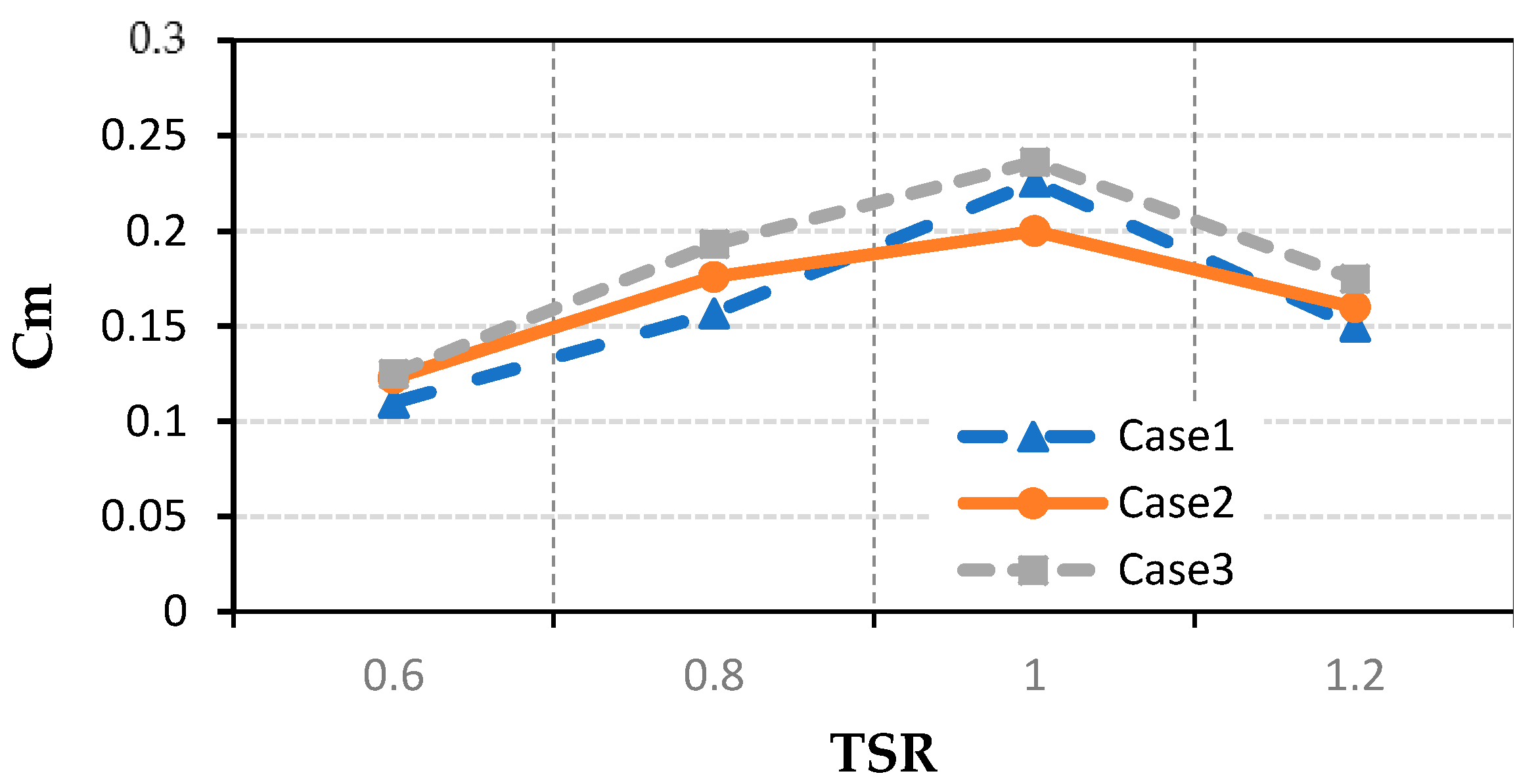
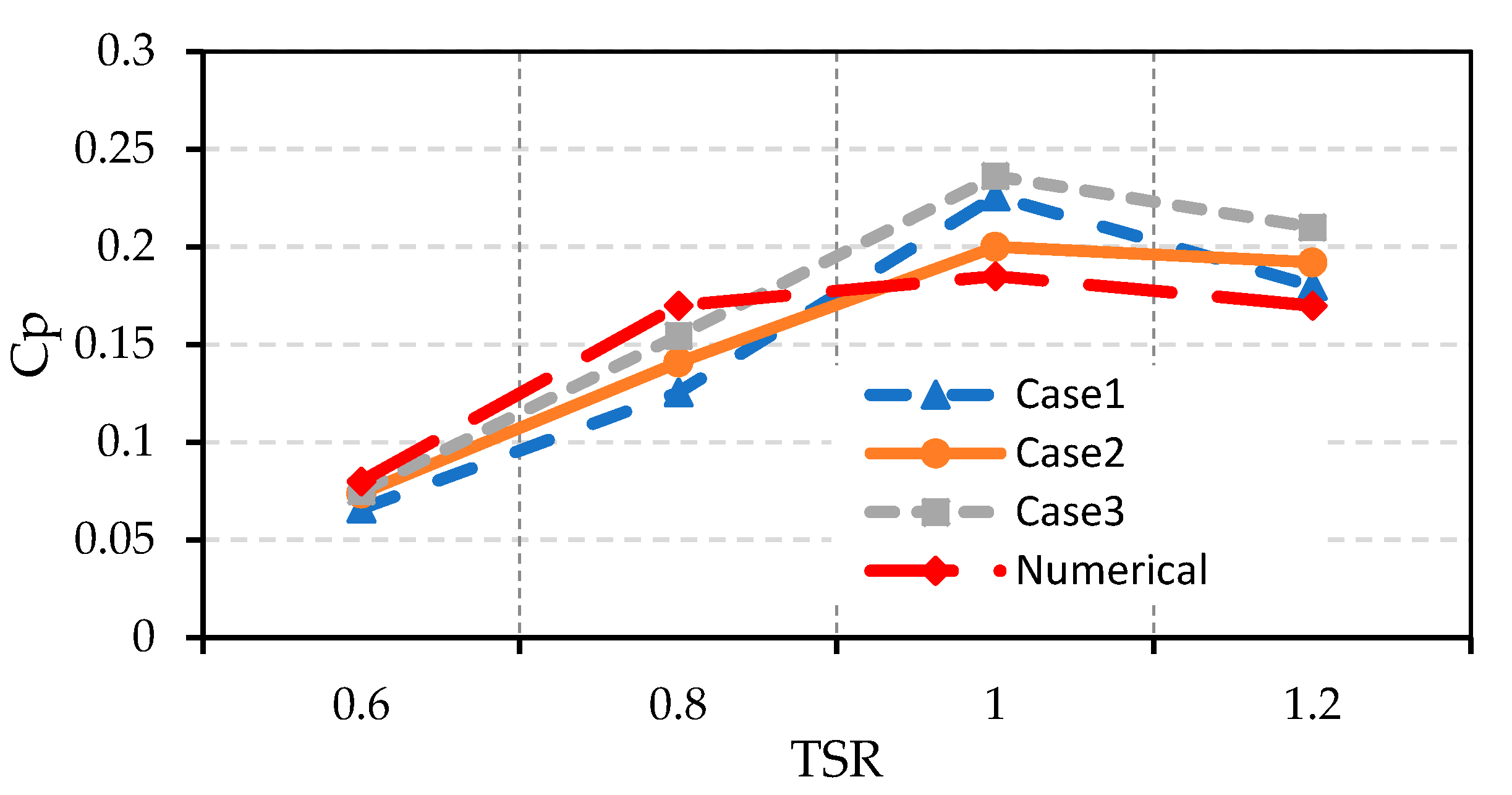
| Tip Speed Ratio | Case 1 | Case 2 | Case 3 | Published Numerical Results [21] | ||||||
|---|---|---|---|---|---|---|---|---|---|---|
| Torque | Cm | Cp | Torque | Cm | Cp | Torque | Cm | Cp | ||
| 0.6 | 8.4964 | 0.11 | 0.066 | 9.48659 | 0.1228 | 0.0736918 | 9.66793538 | 0.12516 | 0.0751 | 0.08 |
| 0.8 | 12.1227 | 0.15694 | 0.12556 | 13.5881 | 0.1759 | 0.1407367 | 14.9248751 | 0.19322 | 0.1545 | 0.17 |
| 1 | 17.4458 | 0.22586 | 0.225866 | 15.448 | 0.2 | 0.2 | 18.2490398 | 0.23626 | 0.23626 | 0.185 |
| 1.2 | 11.586 | 0.15 | 0.18 | 12.3584 | 0.16 | 0.192 | 13.517 | 0.175 | 0.21 | 0.17 |
Publisher’s Note: MDPI stays neutral with regard to jurisdictional claims in published maps and institutional affiliations. |
© 2022 by the authors. Licensee MDPI, Basel, Switzerland. This article is an open access article distributed under the terms and conditions of the Creative Commons Attribution (CC BY) license (https://creativecommons.org/licenses/by/4.0/).
Share and Cite
Ahmed Zaib, M.; Waqar, A.; Abbas, S.; Badshah, S.; Ahmad, S.; Amjad, M.; Rahimian Koloor, S.S.; Eldessouki, M. Effect of Blade Diameter on the Performance of Horizontal-Axis Ocean Current Turbine. Energies 2022, 15, 5323. https://doi.org/10.3390/en15155323
Ahmed Zaib M, Waqar A, Abbas S, Badshah S, Ahmad S, Amjad M, Rahimian Koloor SS, Eldessouki M. Effect of Blade Diameter on the Performance of Horizontal-Axis Ocean Current Turbine. Energies. 2022; 15(15):5323. https://doi.org/10.3390/en15155323
Chicago/Turabian StyleAhmed Zaib, Mansoor, Arbaz Waqar, Shoukat Abbas, Saeed Badshah, Sajjad Ahmad, Muhammad Amjad, Seyed Saeid Rahimian Koloor, and Mohamed Eldessouki. 2022. "Effect of Blade Diameter on the Performance of Horizontal-Axis Ocean Current Turbine" Energies 15, no. 15: 5323. https://doi.org/10.3390/en15155323
APA StyleAhmed Zaib, M., Waqar, A., Abbas, S., Badshah, S., Ahmad, S., Amjad, M., Rahimian Koloor, S. S., & Eldessouki, M. (2022). Effect of Blade Diameter on the Performance of Horizontal-Axis Ocean Current Turbine. Energies, 15(15), 5323. https://doi.org/10.3390/en15155323