1. Introduction
Model Predictive Control (MPC) is a growing field in electrical engineering. Its applications vary widely, from power system control to system management, including wind and solar farms, High-Voltage Direct Current (HVDC) systems, Variable-Speed Drives (VSD), microgrid power management, and multi-level converters [
1,
2,
3,
4,
5,
6,
7].
In particular, Finite-Control Set-MPC (FCS-MPC) is the most popular class of MPC applied to power converters [
8]. This technique presents several advantages, such as a wide bandwidth, fast dynamical response, high disturbance rejection performance, easy inclusion of nonlinearity and constraints, covering several control objectives in power electronics, and easy handling with multi-dimensional and multi-objective control, an essential feature for controlling power converters.
The state-of-the-art of FCS-MPC has already achieved the industrial level for applications such as AC machine control [
9], but for other applications, FCS-MPC still faces a drawback: variable switching frequency that produces a spread switching frequency profile [
10], which is still undetermined quantitatively. There are applications in power electronics that take advantage of variable switching frequency [
11], but they have a fundamental difference from FCS-MPC: these techniques provide a well-determined, i.e., a known, spread profile.
Several works address different solutions for these issues in FCS-MPC [
3,
12,
13,
14,
15,
16,
17,
18,
19,
20,
21]. These studies provided valuable contributions to the field and advanced the state-of-the-art of MPC in power electronics. However, until today, no other work provides a metric to quantify this spread; most analyze only the Total Harmonic Distortion (THD) and the Fast Fourier Transform (FFT), and some use the only metric so far dedicated to characterizing the switching frequency of FCS-MPC: the average switching frequency [
8].
The work presented in this manuscript proposes a new metric to assess the switching frequency spread profile of FCS-MPC based on an instantaneous quantification of the switching frequency of the power converter—this estimation is based on the time that elapses between switching state transitions, that is the time between positive- and negative-edge transitions.
Most of the applications of FCS-MPC use high sampling frequencies, ranging from 10 kHz to 40 kHz [
8,
9,
22,
23], to achieve better power quality and aim to reduce the variability of the sampling frequency, but they usually perform qualitative analyses about the switching frequency [
3,
21].
The investigations performed in this manuscript provide a parametric analysis using this range of sampling frequency to demonstrate the variability of the switching frequency profile, even using high sampling frequencies.
The advantage of the proposed approach is that it estimates the switching frequency instantaneously, which makes it suitable for analyzing the spread spectrum profile of the switching pulses of the power converter using FCS-MPC.
Besides, the analyses using the proposed metric demonstrate that both average switching frequency and THD are insufficient to characterize the switching frequency of FCS-MPC, in contrast with the previous research on FCS-MPC in power electronics; the findings of the work advance the understanding of FCS-MPC switching frequency spread.
The contributions of the work are summarized below:
A new metric designed specifically to evaluate the variability, that is the spread of the switching frequency produced by FCS-MPC;
A quantitative analysis of the switching frequency spread of FCS-MPC supporting the findings;
A discussion about the frequency components—present in the switching frequency profile produced by FCS-MPC—proving that the most common metric, the average switching frequency, is insufficient to characterize the previously mentioned switching frequency profile.
The remainder of this paper is organized as follows:
Section 2 reviews the main contributions in the field concerning the methods to control, analyze, and reduce FCS-MPC switching frequency spread.
Section 3 introduces the new metric and describes its aspects.
Section 4 details the methodology, scope, and objectives of this research.
Section 5 analyzes a set of case studies evaluating the new metric on a converter using a Pulse-Width Modulator (PWM) and a converter using FCS-MPC with two different cost functions.
Section 6 and
Section 7 present the outcomes of the parametric analysis, focusing on the effect of both sampling frequency and cost function weights.
Section 8 discusses the main aspects of the work, followed by the conclusions in
Section 9.
2. Literature Review
FCS-MPC and its variations have been the subject of several types of research in recent years, applied in several branches of power electronics [
2,
24,
25,
26], due to the flexibility that the cost function provides in controlling the variables of interest, besides presenting a transient response superior to linear control [
27].
However, according to [
12], one of the open problems of FCS-MPC is its variable switching frequency, which can even cause resonance problems. The variable switching frequency of FCS-MPC is associated with a widely spread, nonsymmetric, and not well-determined frequency spectrum, making FCS-MPC unsuitable for applications that require strict control of harmonics, such as in grid-connected converters or feeding sensitive loads [
22]. Thus, several works aim to mitigate or control the switching frequency of FCS-MPC. Yet, the papers that somehow quantify the switching frequency do not measure or assess its spread profile, only evaluating its average value.
It is noteworthy that some applications use spread spectrum modulation techniques to reduce Electromagnetic Interference (EMI) [
11], intending to spread the switching frequency spectrum to distribute the energy over a range rather than concentrating it on a single frequency. In other words, such applications take advantage of a spread profile to achieve a valuable feature: EMI reduction.
The difference between these techniques and FCS-MPC—regarding the variable switching frequency—relies on the fact that they use a modulator with a known modulation strategy that spreads the switching frequency within a predetermined range, while FCS-MPC produces a variable, widely spread, and not well-defined switching frequency profile.
The literature has already established that the maximum switching frequency of FCS-MPC is half of the sampling frequency [
2]—with a high spread profile below this maximum value—but misses providing a quantitative method to analyze the spread frequencies.
2.1. Metrics
Currently, the only metric to characterize the switching frequency of FCS-MPC techniques is the average device switching frequency [
8].
Equation (
1) gives the value of the average switching frequency,
, over a determined period equaling
MTs, but this quantity does not measure the variability of the switching frequency in FCS-MPC.
where
M is the total number of samples,
is the sampling period,
is the difference between two consecutive switching states,
is the number of power switches per leg in the power converter under analysis, and
is a correction factor that depends on the converter topology and aims to accomplish the criteria of (
2). For instance, in a two-level three-phase power converter, both
and
are equal to 2.
Another metric used to characterize the power quality of FCS-MPC is the Total Harmonic Distortion (THD), as it quantifies the harmonic content of the current/voltage, given the fundamental frequency component. According to the IEEE-519-2014 standard [
28], THD calculation must consider the harmonic components up to the 50th order (see Equation (
3))—although it may include higher harmonics, if necessary, and consider 12 cycles of the fundamental frequency of 60 Hz.
2.2. State-of-the-Art of FCS-MPC Switching Frequency
One of the first efforts to control the switching frequency in FCS-MPC was described in [
12,
13], where a term was introduced in the cost function to penalize excessive switching state changes. However, this method guarantees neither a fixed switching frequency, nor a deterministic frequency spectrum.
Other strategies were used in [
14,
15] to shape the frequency spectrum of the output variables or mitigate specific harmonics.
The work of [
14] proposes the use of a notch filter in the cost function so that specific harmonic components do not contribute to the cost function value. Even though the proposed method can reduce some harmonics, the switching frequency is still variable. Whereas [
15] uses the Sliding Discrete Fourier Transform (SDFT) method in the cost function to calculate a finite number of components of distinct frequency spectra, assigning weights for each harmonic, nevertheless, as in [
14], reducing some harmonics does not guarantee a fixed switching frequency.
In [
16], the authors replaced the term that minimizes the control effort with a new one that penalizes the deviation between the reference frequency and the estimated frequency. The paper presents valuable contributions, but no further study addresses this method’s impact on the switching frequency.
Other authors sought to include the modulation stage in the optimization process [
17,
18,
19,
20].
The works of [
17,
18] introduce the concept of optimal switching sequence, which formulates the optimization problem as a function of time. In these cases, the variables to be optimized are the switching instants, making the switching frequency fixed, although only unconstrained systems of the type Single-Input–Single-Output (SISO) are suitable for this control strategy.
On the other hand, the methods defined in [
19,
20] take into account the application time of each control signal, synthesizing a Space-Vector PWM (SVPWM), including the modulation scheme within the cost function. However, the optimization process is performed in two steps, increasing the computational effort.
Aiming at a fixed switching frequency method, the authors of [
21] introduced the concept of the Period Control Approach (PCA-MPC), in which the period between two consecutive falling edges and rising edges in the control signal is taken into account, thus being able to compute the frequency. However, it presents a Steady-State Error (SSE) for the desired frequency and adds more complexity to the MPC formulation. The work presented in [
3] solved the problem of the SSE of the frequency by introducing an integrator in conjunction with a fast estimator of the switching frequency. Yet, this method still presents a high degree of complexity in its application.
Two recent papers [
29,
30] studied the effect of different cost functions on a grid-forming converter. These are the most recent studies regarding the switching frequency of FCS-MPC, but both [
29,
30] miss a more rigorous quantification of switching frequency spread.
The work of [
29] analyzes the impact of the cost function on the voltage THD for several operating points using two cost functions without frequency control and two cost functions with frequency control. However, the analysis of the cost function’s impact the switching frequency only qualitatively.
The study presented in [
30] expanded the findings made earlier in [
29], performing an in-depth analysis of how the weights of the cost function and the sampling frequency impact the switching frequency and the THD. However, [
30] use only the average switching frequency as a metric, as other works in the state-of-the-art [
12,
13,
15]. Other works [
14,
16,
17,
18,
20] do not use this metric, evaluating only THD and FFT.
These works significantly contribute to FCS-MPC applications and, directly or indirectly, discuss and propose solutions to the variable switching frequency. They use different techniques to control the switching frequency of FCS-MPC, and most of them have one thing in common: they use the average switching frequency as the only metric to validate the effectiveness of their analysis. However, the results presented in this work will demonstrate in the following sections that this average metric cannot fully characterize FCS-MPC.
3. Total Frequency Spread
The instantaneous switching frequency,
, can be estimated with an algorithm proposed in [
31] (see Algorithm 1), which calculates
based on the time that elapses between switching state transitions, that is the time between positive- and negative-edge transitions.
The work of [
31] applies this method to analyze the switching frequency of hysteresis current controllers in single-phase and three-phase two-level converters.
Now, we propose a new metric, called Total Frequency Spread (TFS), to quantify the spread of the switching frequency profile of power converters, that is the spread of the instantaneous switching frequency,
, provided by Algorithm 1. Algorithm 2, composed of three stages, calculates the TFS.
| Algorithm 1 Switching Frequency Estimator (Based on [31]) |
initialize: initialize: whiledo if positive-edge transition () then else if negative-edge transition () then else end if end while
|
Stage 1 extracts a set of switching frequency components,
, that is the components that
contains, and their distribution
, that is the weight of each component in the switching frequency profile. Equations (
4) and (
5) give these sets; they have the same size,
N , and contain the switching frequency components (
) and their distributions (
), respectively. Note that
M and
N are different values:
M is the total input samples that Algorithm 1 evaluates, and
N is the total number of switching frequency components that Algorithm 2 extracts, after analyzing all
M samples.
For each time instant
, Stage 1 of Algorithm 2 verifies if the instantaneous switching frequency (
) is one of the components of
(given a tolerance); if true, the weight of that component is increased by 1; if not, a new component is added to
with a respective weight equal to 1. At the end of Stage 1, the algorithm normalizes the weights of the switching frequency components
.
Stage 2 of Algorithm 2 calculates a set of auxiliary variables, some necessary to evaluate the TFS in Stage 3; it returns the maximum (
) and minimum (
) switching frequency components in
using Equations (
6) and (
7):
Stage 2 also calculates the dominant frequency,
(Equations (
8) and (
9)), which is the main component of
, that is the component with the highest weight,
, in
:
Stage 3 calculates the TFS using Equation (
10), which computes a squared weighted summation of the quadratic spread between all components in
and the dominant frequency. Then, it normalizes this value using the term
and returns the TFS.
| Algorithm 2 TFS Algorithm |
Stage 1: Extract Switching Frequency Components initialize: for
do for do if then end if end for if is not a component of then end if end for normalization of Stage 2: Calculate Auxiliary Variables Equations ( 4) and ( 5) → Equations ( 6) and ( 7) → Equations ( 8) and ( 9) → Stage 3: Calculate TFS
|
4. Method and Scope
The method of the following analyses uses Equation (
1) to calculate the average switching frequency and Algorithms 1 and 2 to estimate the instantaneous switching frequency and calculate the TFS, respectively. Furthermore, we evaluated the FFT and THD using the IEEE 519-2014 standard [
28]. The analyses’ scope is limited to a three-phase grid-connected converter with AC current control and an LR filter simulated in MATLAB/Simulink, that is the converter topology and the operation levels (see
Table 1) are the same for all case studies and the parametric analysis.
The digital delay of one sampling period observed in real-time applications was also simulated in the models in MATLAB/Simulink; therefore, the FCS-MPC algorithm evaluates the predictions in the time instant
to overcome this issue [
8,
22,
32]; this is a common and the most indicated approach in the state-of-the-art and enhances the simulation models by considering the delay effect in the results.
This work presents a set of five significant analyses that support the findings of this research and validate the proposed metric. These analyses are summarized as follows:
A case study evaluating the proposed metric in a PWM-based converter. The objective of this first analysis is to demonstrate that the components of the switching frequency profile match the FFT of the switching pulses;
A second case study assesses the proposed metric for an FCS-MPC-based converter, which uses only an AC current regulation in the cost function. This analysis illustrates the variability, that is the spread of the switching frequency components in FCS-MPC;
A third case study, similar to the previous one, considers that FCS-MPC operates with an additional term in the cost function to penalize the switching transitions. The objective is to discuss the effectiveness of this cost function in the spread of the switching frequency profile in FCS-MPC;
A discussion about the filter sizing impact on the spread of the switching frequency profile in FCS-MPC;
A parametric analysis that provides insightful findings about the relation between the sampling frequency and the switching frequency components. This analysis sweeps the sampling frequency between a wide range of values—typical in FCS-MPC—these values being integer multiples of the system’s fundamental frequency.
5. Case Studies
The first step of this research is to assess the switching frequency spread of three case studies from the perspective of these metrics:
In Cases 2 and 3, the cost function of FCS-MPC aims to control the converter’s AC currents in the
-frame. Note that Equation (
12) adds a constraint, that is a penalty term—weighted by the parameter
—that penalizes the excessive switching state transitions; this is a common approach in FCS-MPC [
12,
13] that aims to reduce the average switching frequency and the variability of the switching frequency profile. The analysis of Case 3 examines the value of
to determine its impact on the metrics.
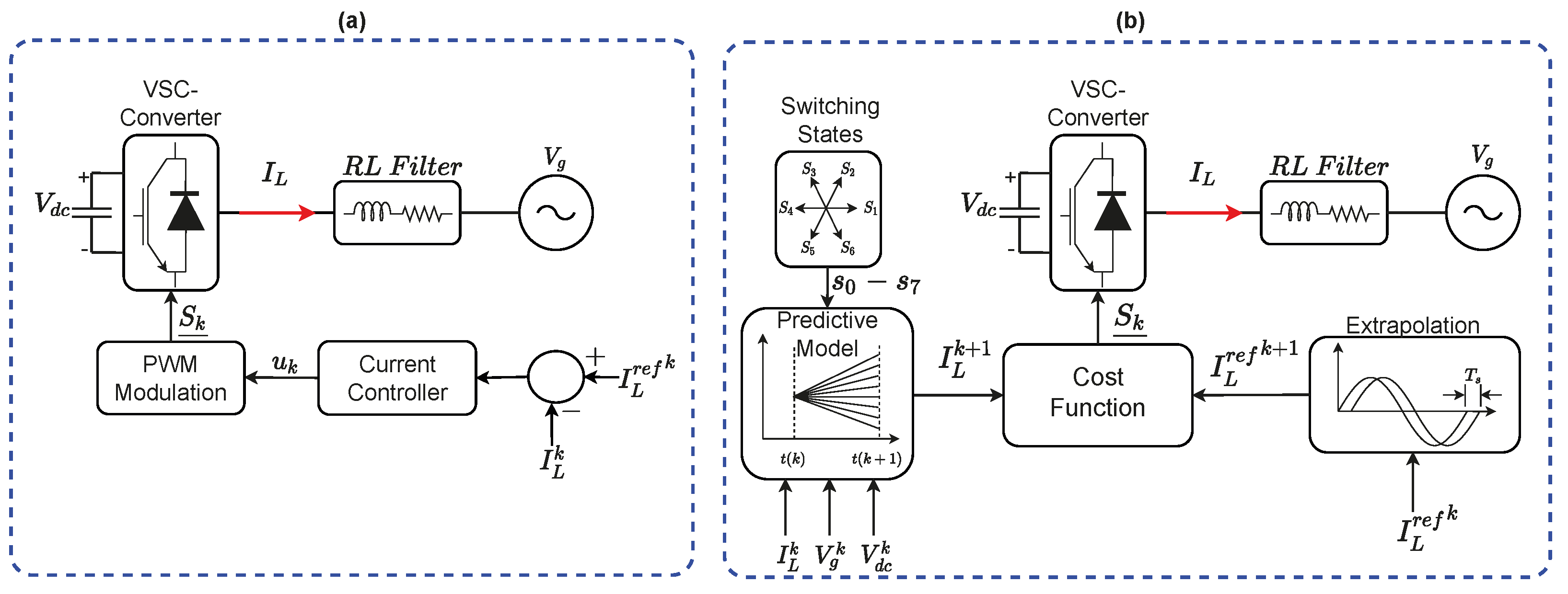
Figure 1 depicts the block diagrams of a PWM-based converter (see (a)—Case Study 1), which produces a fixed switching frequency, and an FCS-MPC based converter (see (b)—Case Studies 2 and 3), which generates a spread switching frequency profile.
5.1. Case 1: PWM-Based Converter
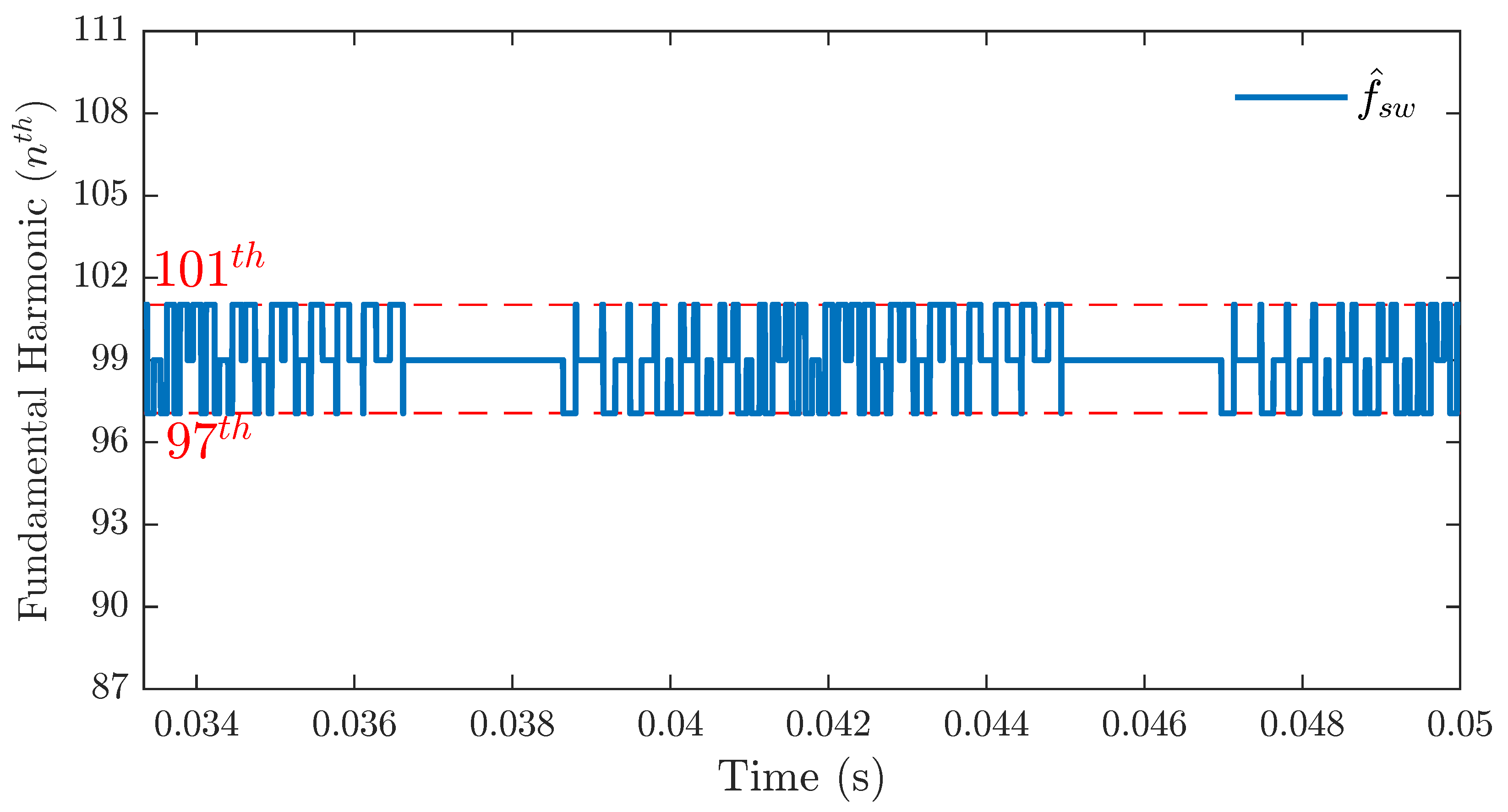
An ideal PWM-based converter operates with a fixed switching frequency. Thus, Algorithm 1 should estimate a constant instantaneous switching frequency when analyzing the switching pulses generated by an ideal PWM.
Figure 2 shows the output of this estimation, which is an instantaneous switching frequency over time equal to the sampling frequency
Hz) oscillating between the range of two fundamental frequency harmonics.
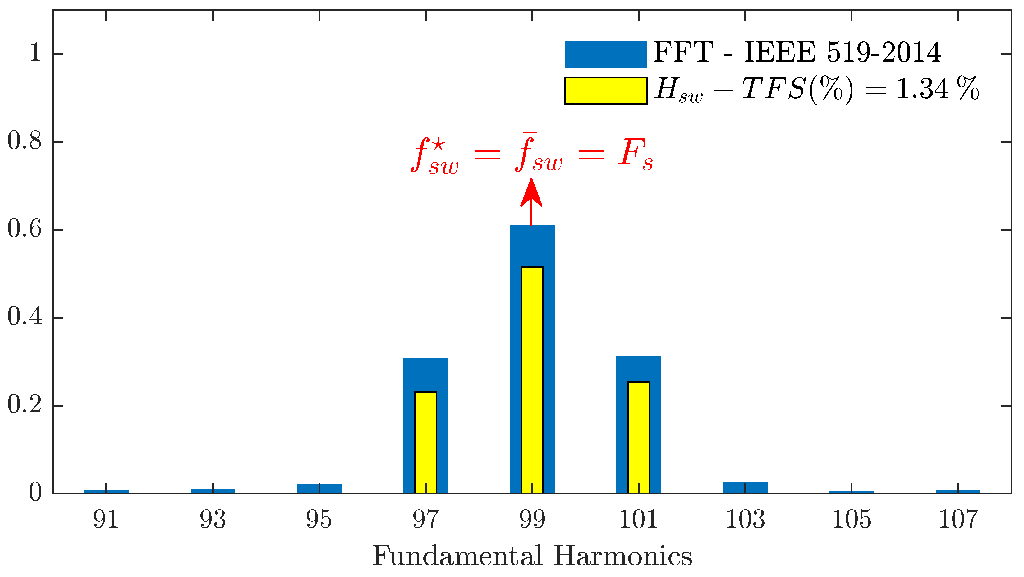
Figure 3 shows that the normalized distribution of the instantaneous switching frequency (
) of
Figure 2 is coherent with the switching pulses’ Fast Fourier Transform (FFT), which contains the modulator switching frequency component
plus the two side lobes
and
.
This result leads to the conclusion that the dominant frequency () of an ideal PWM-based converter is equal to the sampling frequency () and the average switching frequency ().
The components’ amplitudes of both FFT and are different since is a normalized distribution of , that is the percent time that is equal to each component, which is conceptually different from the meaning of the FFT component’s amplitude.
In other words, gives the information of the weight of each switching frequency component, i.e., their normalized ratio over time.
5.2. Case 2: FCS-MPC-Based Converter
Despite presenting fast dynamics and a high disturbance rejection capability, among other features, the classical FCS-MPC generates switching pulses with a high switching frequency spread, that is its switching frequency varies with time [
12].
In this case, we compared FCS-MPC using two different values of sampling frequency; in
Figure 4, the sampling frequency is equal to one of the PWM modules of the previous study case (5940 Hz), and in
Figure 5, we selected a value of
(29,460 Hz) that produces a higher TFS—the sampling frequency effect on the TFS will be detailed in
Section 7.
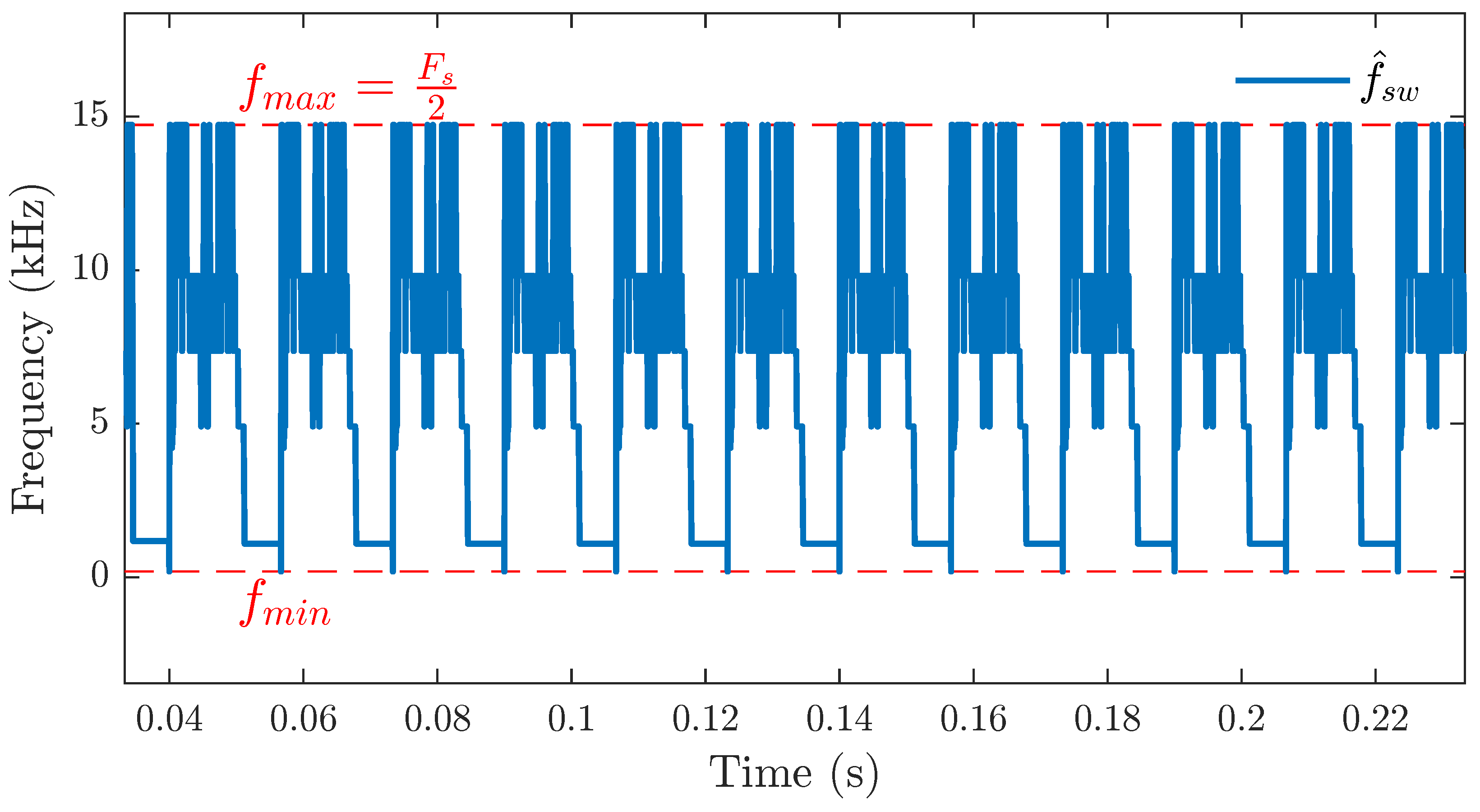
Figure 4 shows the high variability of the instantaneous switching frequency of a classical FCS-MPC, controlling the AC currents of an AFE converter. It ranges from a low switching frequency component (
) to its maximum theoretical value, which equals half of the sampling frequency (
).
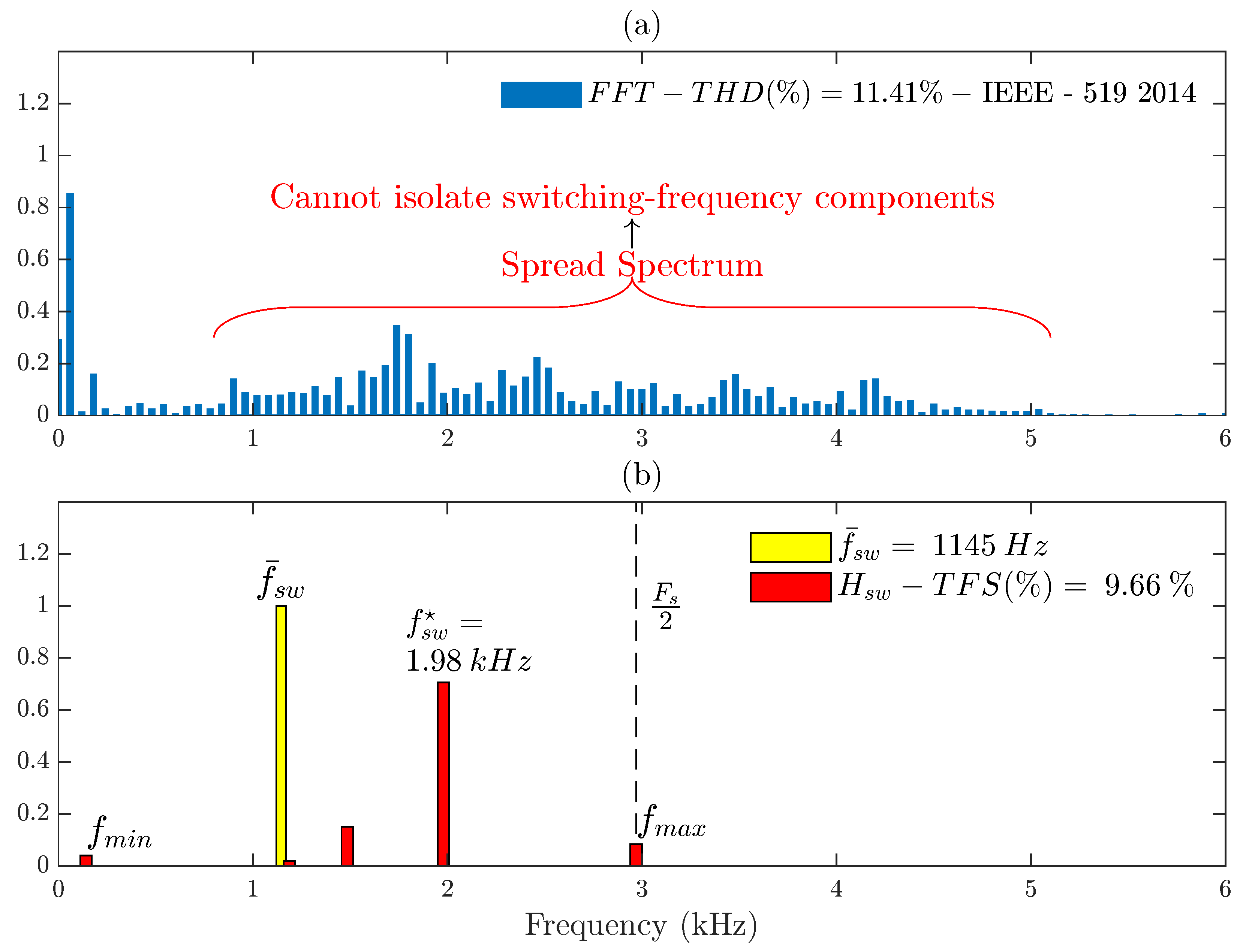
Until now, the study of switching frequency spread in FCS-MPC has been resumed as two methods, whether examining the average switching frequency (yellow bar of
Figure 6b) or the switching pulses’ FFT and current THD, both depicted in
Figure 6a, which shows a spread spectrum making it highly difficult to isolate the switching frequency components, unlike the case of a PWM-based converter.
Now, we can deepen the findings on the switching frequency spread in FCS-MPC by using the proposed metric, TFS. The distribution of the FCS-MPC instantaneous switching frequency, depicted in
Figure 6b, isolates the switching frequency components (in red) and shows that the average switching frequency (in yellow),
, is not even a component of , and it is very distant from the dominant frequency,
—unlike the case of the PWM-based converter, in which both
and
match.
This means that
is only a poor average representation of a highly spread switching frequency profile and cannot fully characterize the switching frequency of FCS-MPC. Moreover, that distribution shows the presence of both maximum and minimum components observed in
Figure 4.
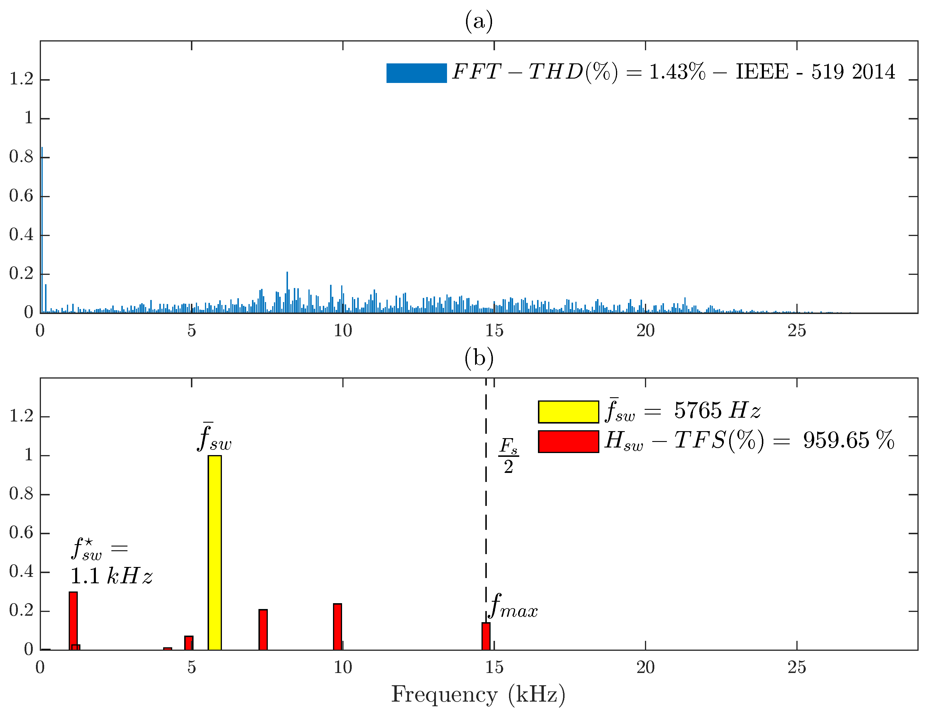
One could argue that the sampling frequency increasing would reduce the switching frequency spread in FCS-MPC, as it naturally decreases THD. However,
Figure 7 proves otherwise: (a) shows the highly spread FFT spectra, but again, we cannot isolate the switching frequency components, as in
Figure 6, again,
is not a component of
, but now, the dominant frequency is the lowest component in
. On the other hand,
Figure 7b shows the switching frequency components—obtained through Algorithm 2—more spread than the case of
Figure 6, highly increasing TFS.
This observation supports the conclusion that increasing the sampling frequency does not reduce TFS, that is the switching frequency spread;
Section 7 extends this finding, concluding that TFS has a nonlinear behavior concerning the sampling frequency.
5.3. Case 3: FCS-MPC with Switching Transition Cost
Adding the number of switch transitions to the cost function is one of the most common approaches [
12] to reduce the switching frequency spread in FCS-MPC. Indeed, it aims to concentrate the switching frequency components within a smaller range. Equation (
12) implements this method, which demands the user to set the weight
. Several works study the effect of
on both THD and
, but without a tool to evaluate the contribution of
to the reduction in the frequency spread [
29,
30].
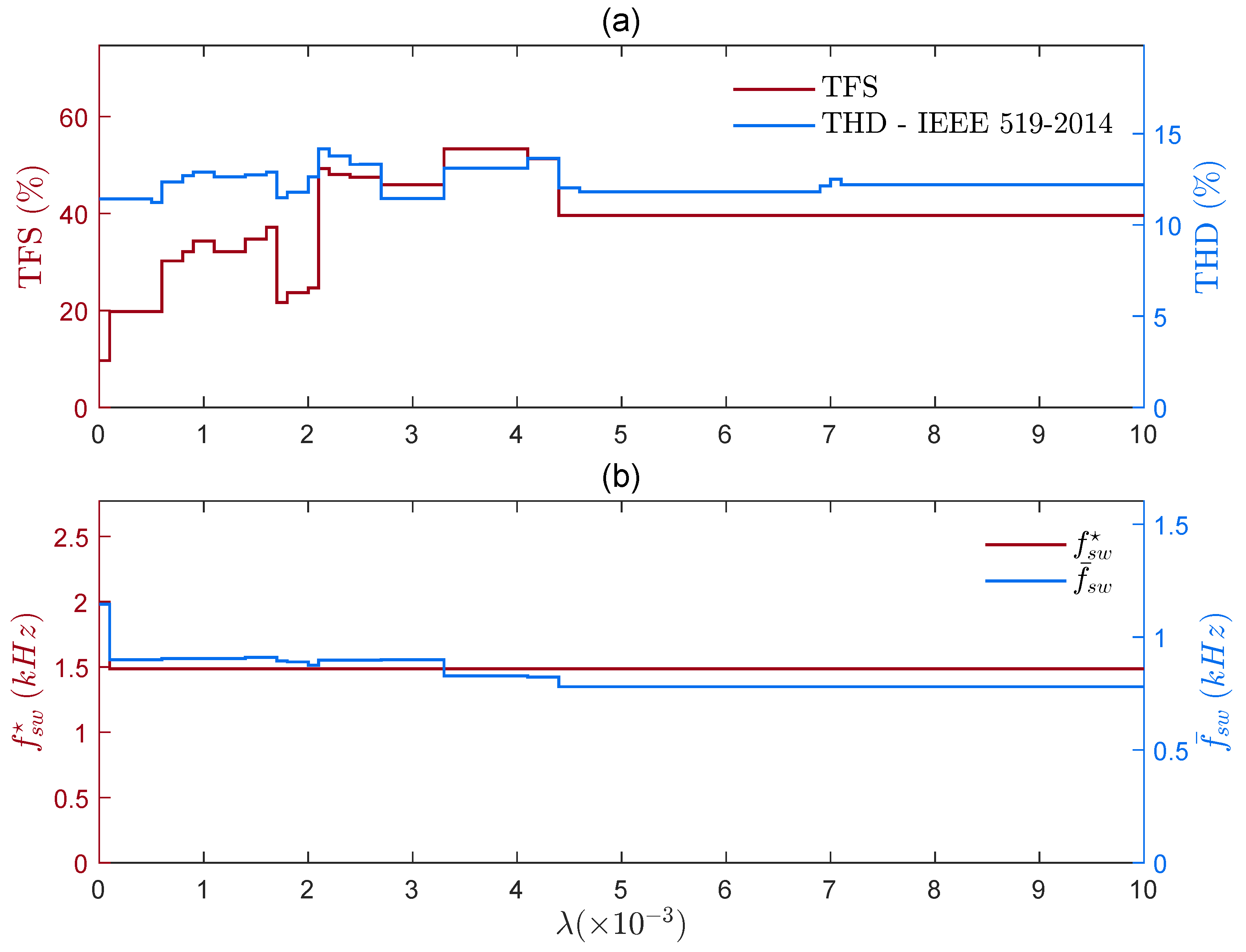
Figure 8 and
Figure 9 compare the effect of
in both TFS and THD, using two different values of the sampling frequency (5940 Hz and 29,460 Hz, respectively)—
equal to zero means the cost function does not consider the switching state transitions. The range of values chosen for the weighting factor to verify its impact on the switching frequency spread was from
to
—typical values encountered in the literature [
8,
13]—being a compromise between the switching frequency reduction term and the current control term in the FCS-MPC cost function.
In the first case (
Hz),
Figure 8a demonstrates that adding the switch transition cost reduces the value of
, but increases THD and TFS, regardless of the value of
. The value of
is constant—but lower than in the case of
equal to zero—and again,
and
are different.
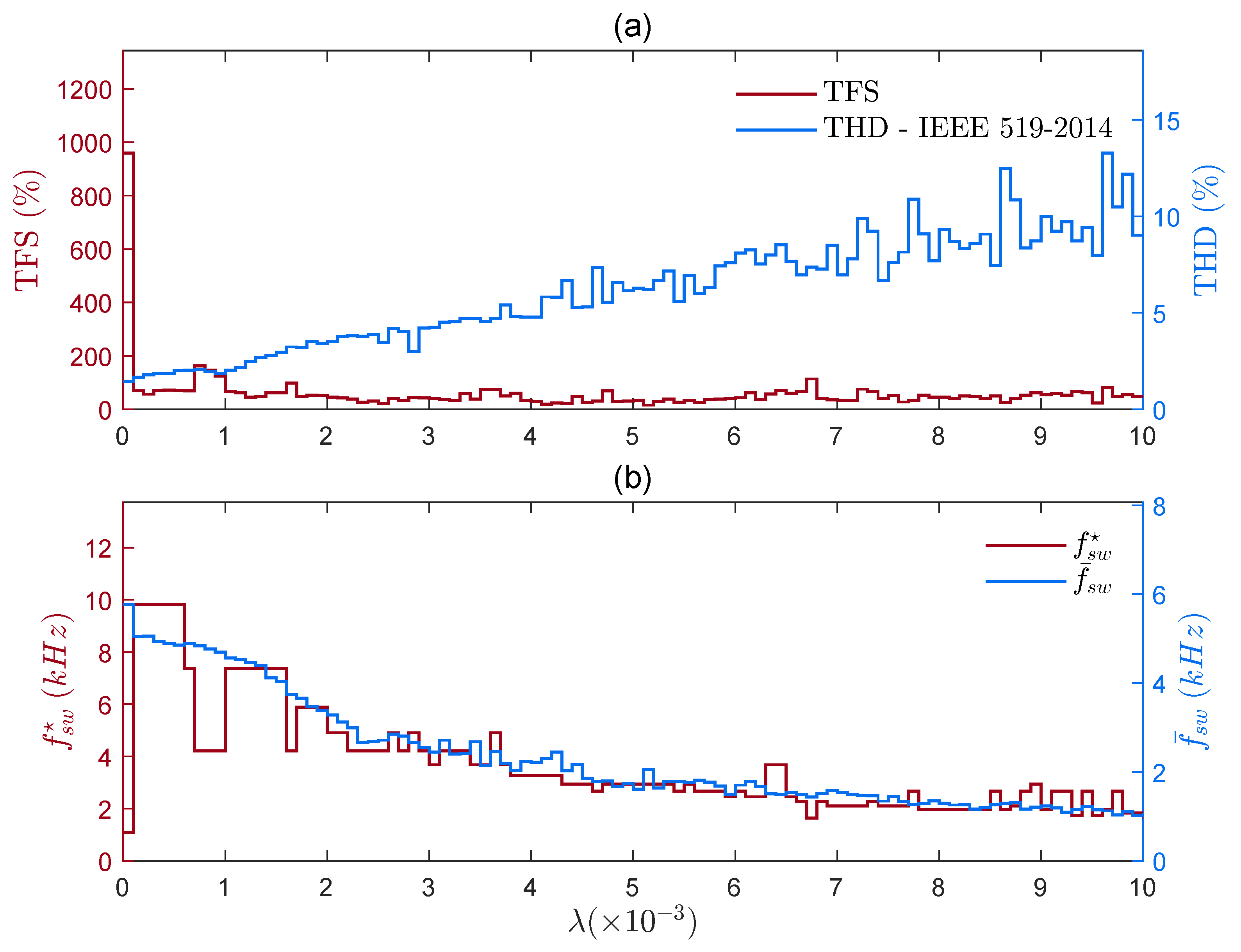
On the other hand, in the case in which
Fs = 29,460 Hz,
Figure 9a shows that increasing the value of
tends to significantly reduce TFS,
, and
. THD increases as expected, but with the help of the proposed metric, one can design the value of
to achieve a reduction in TFS and a THD lower than 5%.
6. Filter Sizing and Setpoint
Filter sizing plays a major role in the resultant THD, as increasing the inductance
L reduces the THD (see
Figure 10a) and the value of
(see (b))—which differs from the value of
, as the value of L increases. However, TFS presents a different behavior: increasing
L does not mean a reduction in TFS (see (a)).
These outcomes reinforce the conclusion that FCS-MPC produces a nonlinear spread switching frequency profile, dependent on the value of L. Therefore, THD and the average switching frequency are insufficient metrics to address or analyze the filter’s design.
On the other hand,
Table 2 provides the TFS value for different operation points, showing a reduction in the spread as the setpoint increases, but for 1.0 pu, TFS rises, again reinforcing the conclusion that FCS-MPC produces a nonlinear switching frequency profile. Indeed, these results, along with those of the other sections, show how difficult it is to design an FCS-MPC solution.
7. Sampling Frequency Effect
The following parametric analyses use the same methodology described in
Section 4, but now, they sweep the value of the FCS-MPC sampling frequency (
Fs), always being an integer multiple
p of the system’s fundamental frequency (
Hz).
7.1. FCS-MPC without Switching Transition Cost
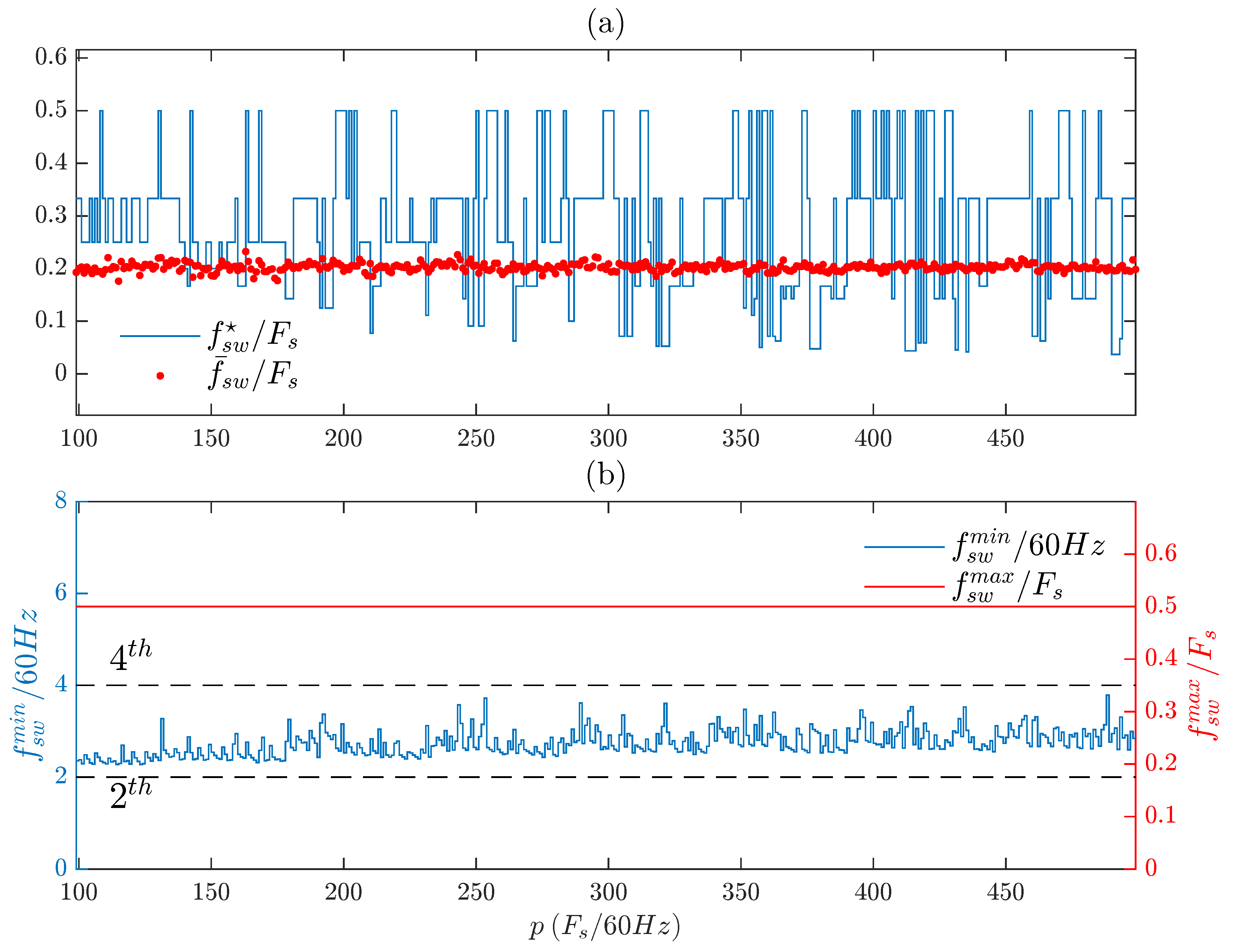
Figure 11a shows that, while
is almost constant in all cases—around
of
Fs—the dominant frequency (
) changes between many levels, which is a nonlinear behavior of FCS-MPC. (b) shows that the maximum component (
) in
is always half of the sampling frequency, which is consistent with the literature in the field [
2,
12]. The value of the lowest component (
) is always between the second and fourth harmonics of the fundamental frequency, regardless of the sampling frequency (
Fs).
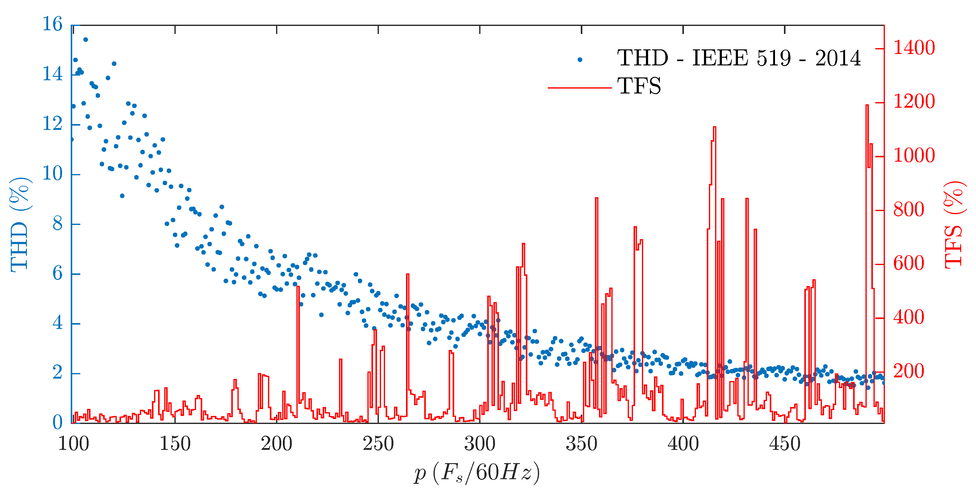
THD presents an overall reduction trend as the sampling frequency increases, as depicted in
Figure 12, although small increments of
Fs can increase THD. These findings are well established in the literature [
8,
22].
However, TFS presents a highly nonlinear behavior with some high peaks, showing that the switching frequency spread profile is highly dependent on the choice of the sampling frequency.
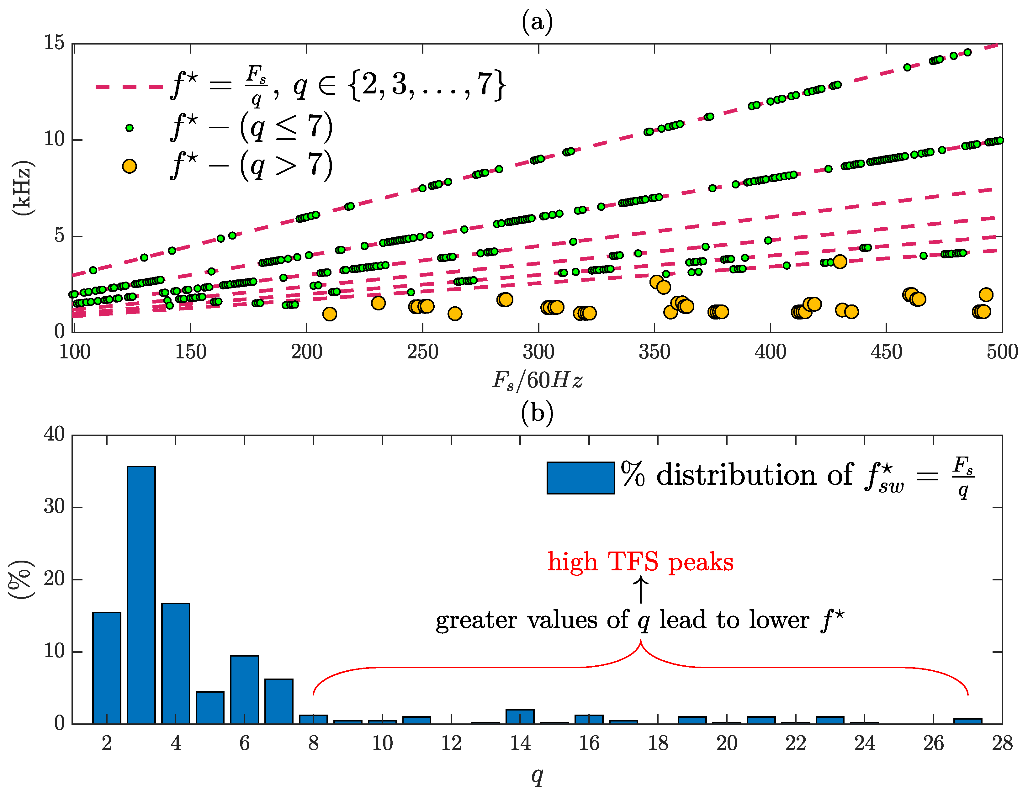
The dominant frequency is an integer fraction of the sampling frequency. As the maximum switching frequency allowed is
, Equation (
13) formalizes that finding.
The outcome of
Figure 13 confirms this finding in (a). In most cases,
q ranges from 2 to 7 (see (b)), but for some sampling frequencies,
q reaches greater values, making
more distant from
, therefore elevating the switching frequency spread—these cases are the reason for the high TFS peaks in
Figure 12.
7.2. FCS-MPC with Switching Transition Cost
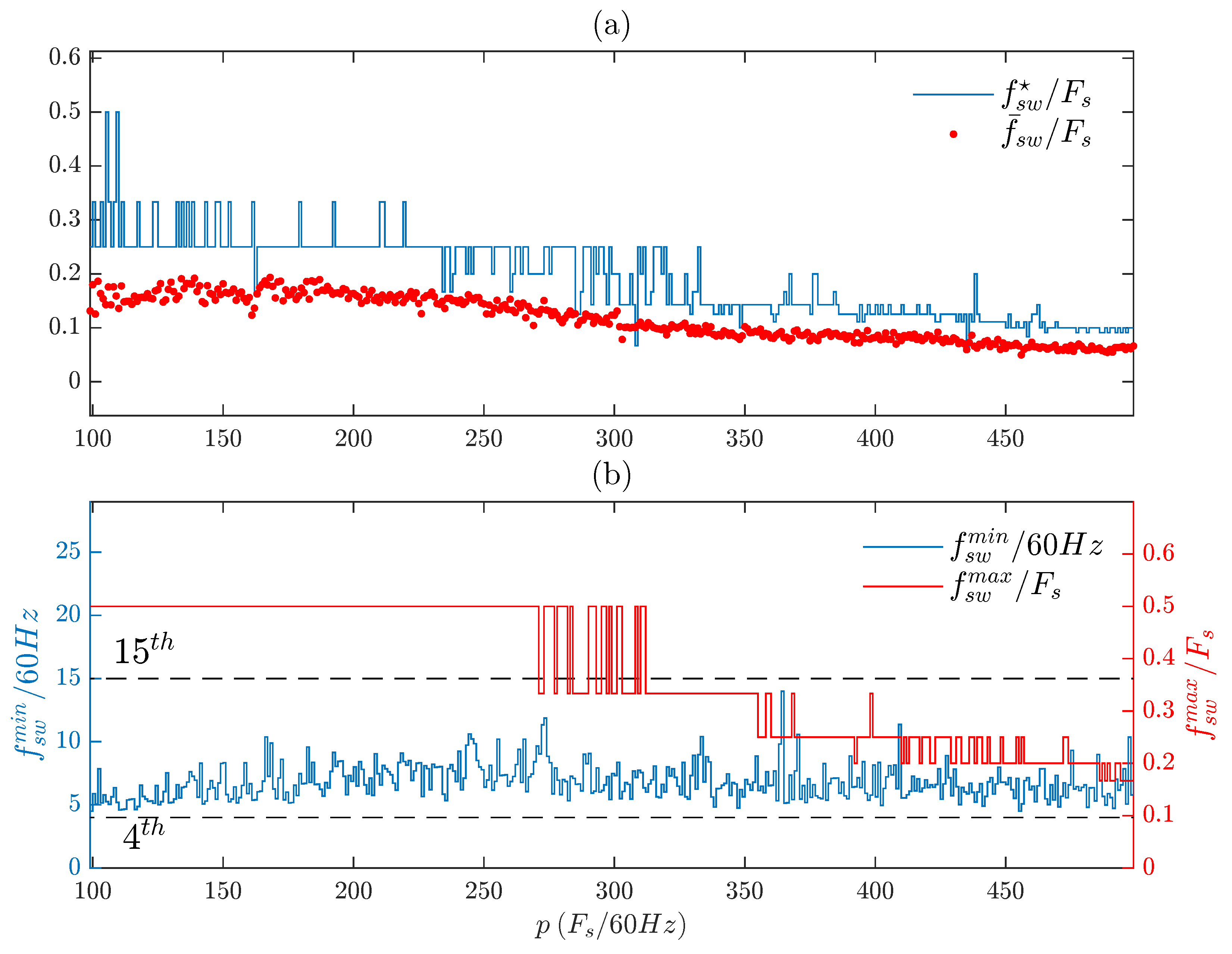
Figure 14 presents the same analysis as
Figure 11, but now, we include the switch transitions in the cost function (using Equation (
12) instead of (
11)).
The switch transitions’ cost reduces the ratio between
and
Fs, as
Fs increases (see
Figure 14a). Moreover, (b) shows that this approach can reduce the maximum frequency
to values below half of
Fs and now makes the minimum frequency in between the
and
harmonics, in contrast to the result of
Figure 11, in which
is always half of
Fs and
is in between the
and
harmonics. Hence, the frequency components of
tend to be more grouped, i.e., less spread.
Figure 15 shows the reduction of those high TFS peaks observed in
Figure 12. This means that using the cost function of (
12)—with a proper selection of
—can reduce TFS, at the cost of a higher THD.
8. Discussion
Choosing the sampling frequency as a multiple integer
p of the fundamental frequency (
Hz) leads to the dominant frequency being proportional to the fundamental frequency by the ratio of
p and
q:
Nothing guarantees that p and q are multiples of each other—which would make the dominant frequency a harmonic component of the fundamental frequency.
Therefore, the dominant frequency will often be a non-characteristic component in the switching frequency profile. In the literature, the average switching frequency is also a non-characteristic component, but this work showed that this average metric is insufficient to assess the spread profile [
13,
16,
27]. Moreover, the dominant frequency is more suitable as a definition of the main switching frequency component.
The maximum switching frequency contributes more to elevating the TFS than the minimum switching frequency since those high TFS peaks occur only in the cases in which the dominant frequency is close to
, therefore more distant from
. This outcome points to a path on which future work can develop strategies—and verify their effectiveness—to bring the dominant frequency closer to the maximum frequency to reduce TFS. To date, the main works in the literature have focused on concentrating qualitatively on the FFT components [
14,
21,
33].
The reduction of the setpoint may cause an increment of the switching frequency spread, although future investigations may deepen this analysis since only a few works approach different operation points regarding the switching frequency in FCS-MPC; for instance, the research of [
20,
23,
34,
35] only analyzes the spectrum of the switching pulse for nominal power.
The works of [
3,
15,
19,
29,
30] applied different control techniques to reduce or control the variable switching frequency. They achieved different levels of success in this task. However, the literature provides only THD and the average switching frequency as their main metrics to verify the effectiveness of the proposed methods. As exposed in this article, these metrics are insufficient to describe the frequency spread profile of FCS-MPC and characterize it completely.
In summary, the state-of-the-art of FCS-MPC provides valuable contributions to the field, but this can only lead to qualitative conclusions regarding the switching frequency spread, in contrast to this work, which presented the first metric to analyze the switching frequency spread of FCS-MPC.
9. Conclusions
TFS has proven to be a game-changing method for analyzing the variability of the switching frequency profile of FCS-MPC, being the first metric in the literature that provides a quantitative assessment of the spread spectrum produced by FCS-MPC techniques.
The outcomes of this work demonstrate that sampling frequency selection highly affects TFS, which leads to the conclusion that increasing the sampling frequency does not ensure a better profile with reduced variability in the switching frequency. However, no analytical model—which could relate the sampling frequency, the TFS, and the dominant frequency—arises from the findings because of the nonlinear behavior of FCS-MPC.
Both THD and average switching frequency are not sufficient metrics to characterize the switching frequency profile of FCS-MPC since they do not fully represent its switching frequency components. On the other hand, the proposed method extracts these components and provides a metric to quantify their spread.
This paper introduced the concept of the dominant frequency, the main component of the instantaneous switching frequency profile; its value differs from the average switching frequency in FCS-MPC-based converters and is an integer fraction of the sampling frequency. This outcome leads to the conclusion that the main switching frequency component of FCS-MPC may not be an integer multiple of the fundamental frequency.
The dominant frequency alone cannot measure the spread of the switching frequency profile, but it is an essential element in TFS evaluation. The analysis of this variable supports the conclusion that the average metric is a poor assessment of FCS-MPC, and the findings of this work proved that the average switching frequency is not even a component in the switching frequency profile.
These conclusions expand the knowledge about FCS-MPC and are a valuable discussion in the field. This work provides important new information about FCS-MPC, and future researchers can now use the TFS and the methods described in this manuscript to advance the analyses of other MPC strategies to quantify the contribution of a wide range of control techniques, such as OSS-MPC, to reduce or control the switching frequency spread. Besides, future works can study filter design, the effect of other filter topologies, and their resonance issues in FCS-MPC by analyzing these subjects using TFS. Furthermore, TFS can be evaluated in contrast with the switching losses to examine the impact of the switching frequency spread on the efficiency of power converters operating with MPC techniques.
Author Contributions
Conceptualization, T.T.; Formal analysis, T.T.; Project administration, M.A.; Writing—original draft, T.T. and J.A.C.; Writing—review & editing, J.A.C., D.H., E.G.-D., J.M.C. and M.A. All authors have read and agreed to the published version of the manuscript.
Funding
This research was funded by the CNPq (National Council for Scientific and Technological Development—Brazil) and by the European Union—NextGenerationEU—University of Seville, grant number MSALAS-2022-19823.
Institutional Review Board Statement
Not applicable.
Informed Consent Statement
Not applicable.
Data Availability Statement
Not applicable.
Acknowledgments
Thanks to the Universidad de Sevilla for the contributions and for providing support from professors and students; to the Federal University of Rio de Janeiro, for providing equipment and physical structure.
Conflicts of Interest
The authors declare no conflict of interest.
Abbreviations
The following abbreviations are used in this manuscript:
| Average switching frequency |
| Instantaneous switching frequency |
| Dominant frequency |
| Sampling period |
| Sampling frequency |
| Minimum switching frequency |
| Maximum switching frequency |
| Weight of the dominant frequency |
| Set of switching frequency components |
| Set of switching frequencies’ weights |
| N | Size of the set of switching frequencies |
| Switching frequency components |
| Switching frequency components’ weights |
| Total Frequency Spread |
References
- Elsisi, M.; Tran, M.Q.; Hasanien, H.M.; Turky, R.A.; Albalawi, F.; Ghoneim, S.S.M. Robust Model Predictive Control Paradigm for Automatic Voltage Regulators against Uncertainty Based on Optimization Algorithms. Mathematics 2021, 9, 2885. [Google Scholar] [CrossRef]
- Vazquez, S.; Franquelo, L.G.; Norambuena, M.; Rivera, M.; Rodriguez, J. Model Predictive Control for Power Converters and Drives: Advances and Trends. IEEE Trans. Ind. Electron. 2016, 64, 935–947. [Google Scholar] [CrossRef] [Green Version]
- Aguirre, M.; Kouro, S.; Rojas, C.A.; Vazquez, S. Enhanced Switching Frequency Control in FCS-MPC for Power Converters. IEEE Trans. Ind. Electron. 2021, 68, 2470–2479. [Google Scholar] [CrossRef]
- Vali, M.; Petrović, V.; Pao, L.Y.; Kühn, M. Model Predictive Active Power Control for Optimal Structural Load Equalization in Waked Wind Farms. IEEE Trans. Control. Syst. Technol. 2022, 30, 30–44. [Google Scholar] [CrossRef]
- Yang, Y.; Yeh, H.G.; Nguyen, R. A Robust Model Predictive Control-Based Scheduling Approach for Electric Vehicle Charging With Photovoltaic Systems. IEEE Syst. J. 2022, 1–11. [Google Scholar] [CrossRef]
- Zhao, Z.; Zhang, J.; Yan, B.; Cheng, R.; Lai, C.S.; Huang, L.; Guan, Q.; Lai, L.L. Decentralized Finite Control Set Model Predictive Control Strategy of Microgrids for Unbalanced and Harmonic Power Management. IEEE Access 2020, 8, 202298–202311. [Google Scholar] [CrossRef]
- Guo, Z.; Li, K.J.; Liu, Z.; Wang, J.; Li, L. A Novel Multistage Model Predictive Control with Reduced Calculation Burden for Modular Multilevel Converters in High Voltage Direct Current System. In Proceedings of the 2021 IEEE International Conference on Predictive Control of Electrical Drives and Power Electronics (PRECEDE), Jinan, China, 18–20 September 2021; pp. 759–764. [Google Scholar] [CrossRef]
- Karamanakos, P.; Geyer, T. Guidelines for the Design of Finite Control Set Model Predictive Controllers. IEEE Trans. Power Electron. 2020, 35, 7434–7450. [Google Scholar] [CrossRef]
- Geyer, T. Model Predictive Control of High Power Converters and Industrial Drives; Wiley: Hoboken, NJ, USA, 2016. [Google Scholar]
- Papafotiou, G.A.; Demetriades, G.D.; Agelidis, V.G. Technology Readiness Assessment of Model Predictive Control in Medium- and High-Voltage Power Electronics. IEEE Trans. Ind. Electron. 2016, 63, 5807–5815. [Google Scholar] [CrossRef]
- Gamoudi, R.; Elhak Chariag, D.; Sbita, L. A Review of Spread-Spectrum-Based PWM Techniques—A Novel Fast Digital Implementation. IEEE Trans. Power Electron. 2018, 33, 10292–10307. [Google Scholar] [CrossRef]
- Jose Rodriguez, P.C. Predictive Control of Power Converters and Electrical Drives; Wiley: Hoboken, NJ, USA, 2012. [Google Scholar]
- Vargas, R.; Cortes, P.; Ammann, U.; Rodriguez, J.; Pontt, J. Predictive Control of a Three-Phase Neutral-Point-Clamped Inverter. IEEE Trans. Ind. Electron. 2007, 54, 2697–2705. [Google Scholar] [CrossRef]
- Cortes, P.; Rodriguez, J.; Quevedo, D.E.; Silva, C. Predictive Current Control Strategy With Imposed Load Current Spectrum. IEEE Trans. Power Electron. 2008, 23, 612–618. [Google Scholar] [CrossRef]
- Aggrawal, H.; Leon, J.I.; Franquelo, L.G.; Kouro, S.; Garg, P.; Rodríguez, J. Model predictive control based selective harmonic mitigation technique for multilevel cascaded H-bridge converters. In Proceedings of the IECON Proceedings (Industrial Electronics Conference), Melbourne, Australia, 7–10 November 2011; pp. 4427–4432. [Google Scholar]
- Stellato, B.; Geyer, T.; Goulart, P.J. High-Speed Finite Control Set Model Predictive Control for Power Electronics. IEEE Trans. Power Electron. 2017, 32, 4007–4020. [Google Scholar] [CrossRef] [Green Version]
- Vazquez, S.; Marquez, A.; Aguilera, R.; Quevedo, D.; Leon, J.I.; Franquelo, L.G. Predictive Optimal Switching Sequence Direct Power Control for Grid-Connected Power Converters. IEEE Trans. Ind. Electron. 2015, 62, 2010–2020. [Google Scholar] [CrossRef] [Green Version]
- Vazquez, S.; Aguilera, R.P.; Acuna, P.; Pou, J.; Leon, J.I.; Franquelo, L.G.; Agelidis, V.G. Model Predictive Control for Single-Phase NPC Converters Based on Optimal Switching Sequences. IEEE Trans. Ind. Electron. 2016, 63, 7533–7541. [Google Scholar] [CrossRef]
- Tarisciotti, L.; Zanchetta, P.; Watson, A.; Clare, J.; Bifaretti, S.; Rivera, M. A new predictive control method for cascaded multilevel converters with intrinsic modulation scheme. In Proceedings of the IECON Proceedings (Industrial Electronics Conference), Vienna, Austria, 10–14 November 2013; pp. 5764–5769. [Google Scholar]
- Donoso, F.; Mora, A.; Cardenas, R.; Angulo, A.; Saez, D.; Rivera, M. Finite-Set Model-Predictive Control Strategies for a 3L-NPC Inverter Operating With Fixed Switching Frequency. IEEE Trans. Ind. Electron. 2018, 65, 3954–3965. [Google Scholar] [CrossRef]
- Aguirre, M.; Kouro, S.; Rojas, C.A.; Rodriguez, J.; Leon, J.I. Switching Frequency Regulation for FCS-MPC Based on a Period Control Approach. IEEE Trans. Ind. Electron. 2018, 65, 5764–5773. [Google Scholar] [CrossRef]
- Karamanakos, P.; Liegmann, E.; Geyer, T.; Kennel, R. Model Predictive Control of Power Electronic Systems: Methods, Results, and Challenges. IEEE Open J. Ind. Appl. 2020, 1, 95–114. [Google Scholar] [CrossRef]
- Bordons, C.; Montero, C. Basic Principles of MPC for Power Converters: Bridging the Gap Between Theory and Practice. IEEE Ind. Electron. Mag. 2015, 9, 31–43. [Google Scholar] [CrossRef]
- Kouro, S.; Perez, M.A.; Rodriguez, J.; Llor, A.M.; Young, H.A. Model Predictive Control: MPC’s Role in the Evolution of Power Electronics. IEEE Ind. Electron. Mag. 2015, 9, 8–21. [Google Scholar] [CrossRef]
- Rodriguez, J.; Cortes, P.; Kennel, R.; Kazrnierkowski, M. Model predictive control—A simple and powerful method to control power converters. In Proceedings of the 2009 IEEE 6th International Power Electronics and Motion Control Conference, Wuhan, China, 17–20 May 2009; IEEE: Piscataway, NJ, USA, 2009; Volume 56, pp. 41–49. [Google Scholar]
- Rodriguez, J.; Kazmierkowski, M.P.; Espinoza, J.R.; Zanchetta, P.; Abu-Rub, H.; Young, H.A.; Rojas, C.A. State of the Art of Finite Control Set Model Predictive Control in Power Electronics. IEEE Trans. Ind. Inform. 2013, 9, 1003–1016. [Google Scholar] [CrossRef]
- Young, H.A.; Perez, M.A.; Rodriguez, J.; Abu-Rub, H. Assessing Finite-Control-Set Model Predictive Control: A Comparison with a Linear Current Controller in Two-Level Voltage Source Inverters. IEEE Ind. Electron. Mag. 2014, 8, 44–52. [Google Scholar] [CrossRef]
- Committee, D.; Power, I.; Society, E. IEEE Recommended Practices and Requirements for Harmonic Control in Electrical Power Systems; IEEE: Piscataway, NJ, USA, 2014; Volume 2014. [Google Scholar]
- Alhasheem, M.; Blaabjerg, F.; Davari, P. Performance assessment of grid forming converters using different finite control set model predictive control (FCS-MPC) algorithms. Appl. Sci. 2019, 26, 3513. [Google Scholar] [CrossRef] [Green Version]
- Alhasheem, M.; Abdelhakim, A.; Blaabjerg, F.; Mattavelli, P.; Davari, P. Model predictive control of grid forming converters with enhanced power quality. Appl. Sci. 2020, 10, 6390. [Google Scholar] [CrossRef]
- Caicedo, J.; Aredes, M.; Watanabe, E.H. Frequency analysis behavior of hysteresis current control in VSI. In Proceedings of the 2013 Power Electronics and Power Quality Applications, PEPQA 2013—Proceedings, Bogota, Colombia, 6–7 July 2013; Volume 2. [Google Scholar]
- Venkata Yaramasu, B.W. Model Predictive Control of Wind Energy Conversion Systems; Wiley: Hoboken, NJ, USA, 2017. [Google Scholar]
- Tarisciotti, L.; Zanchetta, P.; Watson, A.; Bifaretti, S.; Clare, J.C. Modulated Model Predictive Control for a Seven-Level Cascaded H-Bridge Back-to-Back Converter. IEEE Trans. Ind. Electron. 2014, 61, 5375–5383. [Google Scholar] [CrossRef]
- Li, X.; Peng, T.; Dan, H.; Zhang, G.; Tang, W.; Wheeler, P. A modulated model predictive control scheme for the brushless doubly-fed induction machine. In Proceedings of the 2017 IEEE Energy Conversion Congress and Exposition (ECCE), Cincinnati, OH, USA, 1–5 October 2017; pp. 1338–1342. [Google Scholar] [CrossRef]
- Rivera, M.; Morales, F.; Baier, C.; Muñoz, J.; Tarisciotti, L.; Zanchetta, P.; Wheeler, P. A modulated model predictive control scheme for a two-level voltage source inverter. In Proceedings of the 2015 IEEE International Conference on Industrial Technology (ICIT), Seville, Spain, 17–19 March 2015; pp. 2224–2229. [Google Scholar] [CrossRef]
| Publisher’s Note: MDPI stays neutral with regard to jurisdictional claims in published maps and institutional affiliations. |
© 2022 by the authors. Licensee MDPI, Basel, Switzerland. This article is an open access article distributed under the terms and conditions of the Creative Commons Attribution (CC BY) license (https://creativecommons.org/licenses/by/4.0/).


 ,
, 


