An Efficient Estimation of Wind Turbine Output Power Using Neural Networks

Abstract

Wind energy is a valuable source of electric power as its motion can be converted into mechanical energy, and ultimately electricity. The significant variability of wind speed calls for highly robust estimation methods. In this study, the mechanical power of wind turbines (WTs) is successfully estimated using input variables such as wind speed, angular speed of WT rotor, blade pitch, and power coefficient (Cp). The feed-forward backpropagation neural networks (FFBPNNs) and recurrent neural networks (RNNs) are incorporated to perform the estimations of wind turbine output power. The estimations are performed based on diverse parameters including the number of hidden layers, learning rates, and activation functions. The networks are trained using a scaled conjugate gradient (SCG) algorithm and evaluated in terms of the root mean square error (RMSE) and mean absolute percentage error (MAPE) indices. FFBPNN shows better results in terms of RMSE (0.49%) and MAPE (1.33%) using two and three hidden layers, respectively. The study indicates the significance of optimal selection of input parameters and effects of changing several hidden layers, activation functions, and learning rates to achieve the best performance of FFBPNN and RNN.

1. Introduction

Electricity is a major infrastructural prerequisite for developing nations and a key factor in most human activities. Electrical energy can help flourish many other sectors such as food, health, education, security, transportation, and industrial production. Modern energy services are a vital driving force for economic development toward sustainable growth. The more efficiently a developing country is able to utilize available energy, the faster it will grow and achieve overall better progress. That is why the socioeconomic development of a nation is measured by per capita energy utilization. Statistically, 73.8% of global electricity output in 2018–2019 was from non-renewable energy sources, while only 26.2% from renewable sources [1]. However, the trend toward clean energy is on a steady rise these days. In 2019, a high annual increase was recorded globally in renewable energy generation—almost 181 GW [2]. Most of the mentioned percentage of renewable electricity was obtained from hydropower which generated 15.8%, with other sources including wind 5.5%, bio-power 2.2%, solar-PV 2.4%, and 0.4% from geothermal and concentrated solar power (CSP) [3].

Wind is the most abundantly available natural energy resource, present everywhere and waiting to be harvested, providing the most reliable option for clean energy production [4]. Wind speed and wind power can be estimated accurately if an appropriate dataset is available. The accuracy of wind speed and wind power estimation depends upon the quality of past data on wind speed and wind power at the given wind turbine (WT) site. The accurate estimation of WT output power requires careful consideration of stochastic factors such as wind speed and power coefficient (C_P). Different input factors are considered in the estimation, including wind speed, wind direction, temperature, air density, etc., but C_P has not been considered by most of the researchers. The main purpose of this study is to accurately estimate WT power output based on maximal stochastic factors. Wind energy is cheap and environment friendly. But efficiently use of wind as a viable source of energy requires accurate estimates of annual power output (kWh per year) to determine whether a particular WT will produce sufficient electricity to meet the relevant energy demand. Such estimations prove extremely helpful in power generation planning and energy management. They are also indispensable in the efforts to replace conventional non-renewable energy resources with multi-GW wind farms. However, the quality of such estimations depends on the availability of reliable and comprehensive data for the given WT site. Erroneous estimates due to unreliable datasets or wrong methodology can be detrimental to correct load management. Different input factors are used in the context of WT output power estimation, e.g., wind speed, air pressure, temperature, air density, WT characteristic curve, etc.

There are three primary types of methods of power estimation: physical, statistical, and learning [5,6,7]. Physical methods rely on weather modeling to estimate effective wind speeds and then use WT characteristic curves for wind power estimation. However, this method requires considerable computation due to its computational complexity. Statistical methods use historical wind data, but this method is only effective for small datasets and a limited number of inputs. Learning methods establish the relationship between inputs and outputs using artificial intelligence, which makes these methods very useful and highly effective. Different deep learning algorithms are developed for this purpose and are widely used in a variety of applications [8].

Several software solutions have been developed to study WT characteristics and behavior in different weather conditions using simulations and soft-computing algorithms. For instance, Jinhua Zhang et al. [9] proposed a long short-term memory (LSTM) network algorithm using a deep learning network for short-term estimation of the output power of three WTs and used a Gaussian Mixture Model (GMM) for the uncertainty analysis of the WTs power while using wind speed and wind direction as input factors. A short-term network was trained in [9] and employed the expectation-maximization (EM) algorithm for the estimation of parameters that were then used by the GMM. RNN was used for wind power estimation by Z. O. Olaofe et al. [10], who estimated wind power generation in real-time over the one-hour horizon of up to 288 h ahead based on the time series data on a 1.3 megawatt (MW) WT, obtained from a 50 m hub, and using wind speed, wind direction, temperature, atmospheric pressure, wind distribution, and WT characteristic curve as input parameters. In [10], the authors first calculated the electric power output of the WT generator relative to the efficiency of gearbox and generator, and then utilized the WT characteristic curve for the estimation. It is pertinent to mention that wind speed is the most used input parameter in wind power estimation because WT output power depends upon the cube of wind speed [6].

In [11], Iulian Munteanu et al. used a 24-h model-based wind park simulator to estimate the output power of an off-shore wind farm. The data used in the study was collected by meteorological masts, and the stochastic input parameters used in the estimation were wind speed and wind direction. The wake effect and effective wind speed for every turbine were considered while estimating the output power of each WT. However, [8] made assumptions about certain parameters including the location of the WTs, the effect of park wakes, wind speed, pitch angle, and wind power. M. Hayashi et al. [9] first estimated the wind speed, and then used that data to project WT power output using the Jacobian Matrix Estimation Method (JMEM). The time series analysis and estimation were done using the deterministic chaos approach (chaos fractal). The data structure was analyzed using fractal dimensional analysis and Lyapunov spectrum analysis. Another study [12] used historical wind speed data collected from multiple areas around the targeted WT site and estimated wind speeds for periods from several hours to up to 24 h ahead. Next, the data were used along with the WT power curve for the estimation of the WT output power. As wind speed increases with altitude, the data used for the estimation of any WT’s output power should be in accordance with its hub height.

In [13], a sparsified vector auto-regressive (VAR) model was introduced by Miao He et al. for the short-term estimation of a wind farm’s output power in a multivariate time series model developed by VAR for wind power generation. The sparse structure of the autoregressive coefficient matrix was taken into account while obtaining the parameters of the VAR model based on the most likely estimation of real-time measurement data. The authors of [13] considered the hub height of a WT while collecting data and used wind speed and wind direction at that height to improve their estimation. They compared their results with autoregressive (AR) and multiple autoregressive (MAR) models and measured the accuracy of singular estimations relative to the mean absolute error (MAE), MAPE, and RMSE, and used continuous rank probability score (CRPS) for probability estimations. Saeed Zolfaghari et al. [14] suggested that the estimation of a WT’s power output yields several inaccuracies if the characteristic curve provided by the manufacturer is used. Hence, they proposed a new method employing power probability distribution functions (PPDFs) instead of the characteristic curve when estimating the output power of a WT. First, the PPDFs-based actual data on speed and corresponding wind power for each WT is used to calculate the individual output power. Then, the output power of the wind farm is computed probabilistically by assigning statistical spatial distribution (i.e., Poisson distribution) for wind speeds over the wind farm based on the calculated PPDFs.

A method of short-term estimation of wind power was suggested by Shuang Hu et al. [15], in which multivariate variables such as wind speed, wind direction, temperature, and air pressure were converted into low dimensional variables using a principal component analysis (PCA) to obtain a simplified network. Then, Elman artificial networks were used to train and optimize the network path, and final estimations were calculated. M. M. BA et al. [16] measured wind speed frequency distribution using Weibull probability density function and assessed wind speeds based on experimental data collected over five years and estimated the output power of small WTs in urban areas. The authors used raw data on wind speed and wind direction recorded using data loggers, which they then compared to experimental results using RMSE. Mantas Marciukaitis et al. [17] used five months of data on the direction and speed of wind to determine a WT power curve using a non-linear regression model and concluded that wind direction was not a significant factor in terms of accuracy of the estimation [17].

In [18], 24-h input data on wind speed and power measured in 10-min intervals were used by G.W. Chang et al. for short-term estimation of wind speed and wind farm power, which employed an improved radial basis function neural network-based model with an error feedback (IRBFNN-EF) scheme. They verified the accuracy of the method using MAPE and RMSPE, and compared their results with other neural network methods. In [19,20], Aamer Bilal Asghar et al. used aerodynamic simulations in FAST code, and estimated WT C_P and effective wind speed, respectively, using TSR, β, and rotor speed as input parameters processed in an adaptive neuro-fuzzy inference system (ANFIS). In [21], the author estimated optimal rotor speed for MPPT of a variable-speed WT using previously estimated effective wind speed.

As follows from the above analysis, WT mechanical power has already been well explored and estimated using input factors such wind speed, wind direction, WT characteristic curve, temperature, pressure, and wind distribution. There is no doubt that wind speed is the most important factor in the calculation of the WT mechanical power as the output power is directly proportional to the cube of wind speed. However, as wind speed data is recorded by an anemometer placed on the nacelle, the wind reaching the anemometer is turbulent as it first passes through the WT blades. Thus, the recorded wind speed data cannot be considered highly accurate. The same goes for wind direction, because wind direction data are recorded by a wind vane which is also placed over the nacelle, beside anemometer, and faces the turbulent wind coming from the WT blades. WT characteristic curve is also unreliable in terms of WT output power estimation as such information is provided by the WT manufacturer and gathered in controlled environmental conditions, without considering any practical issues such as stochastic weather conditions that may include wind gusts and sudden variations in wind speed [22].

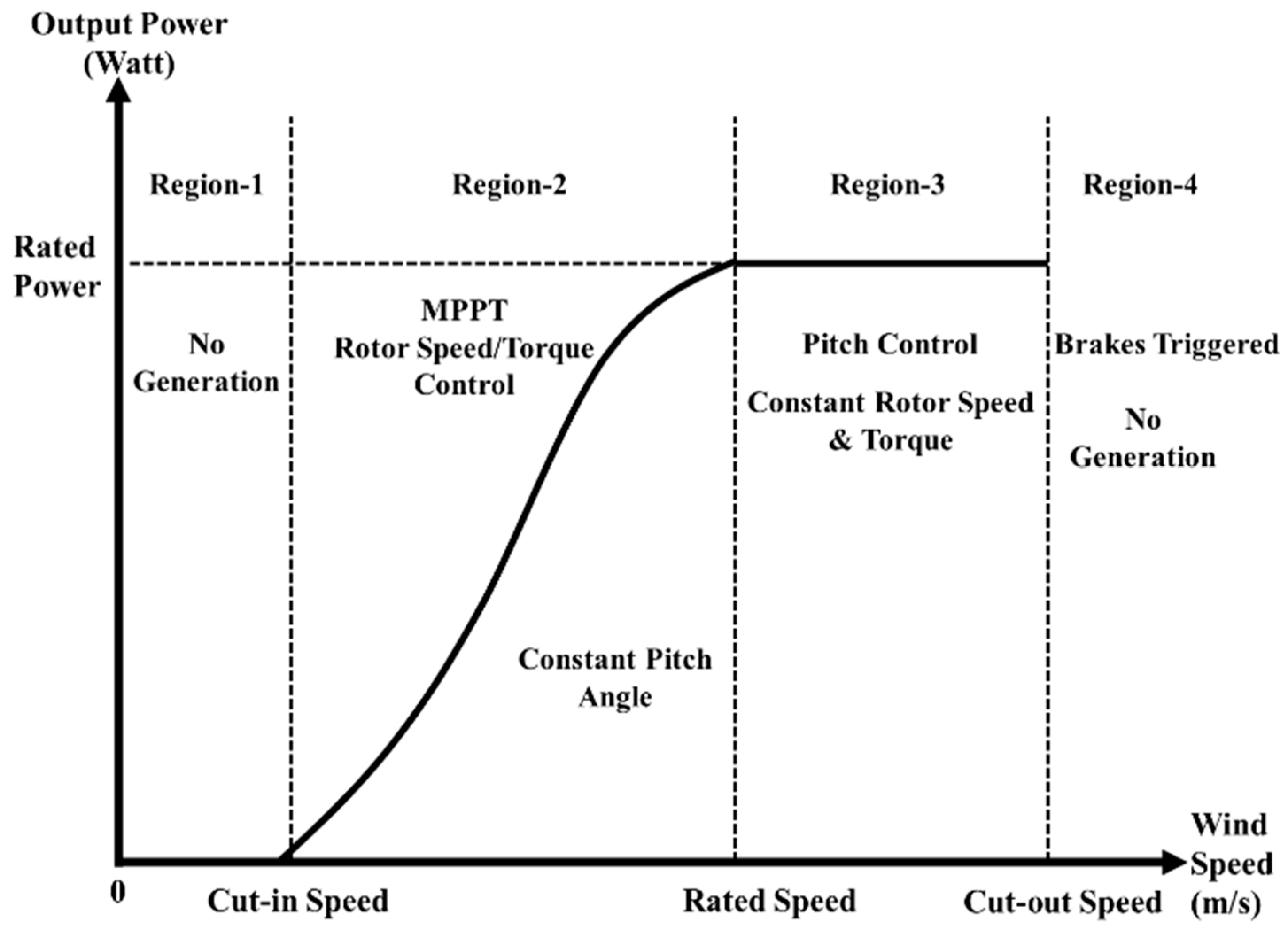
Incident wind power depends on air density, rotor swept area, and the cube of effective wind speed. A WT converts this incident wind power into mechanical power, where the ratio of this mechanical power and incident power is C_P and never exceeds a certain limit. The power coefficient is expressed as a non-linear function of tip speed ratio (TSR) and collective blade pitch angle (β). TSR is the ratio of the instantaneous velocity of the rotor blade tip to the wind speed. C_P reaches its maximum value C_Pmax at the optimum value of TSR (λ_opt), i.e., the optimal operating point of the WT. This means that a change in wind speed can cause a change in TSR and β, which in turn can affect C_P.

It can therefore be concluded that the mechanical power of a WT depends on two variables that are constantly changing, i.e., wind speed and C_P. This is exactly why the WT output power is so difficult to estimate and why electricity generated by WTs is relatively hard to manage. The accuracy of wind speed and wind power estimations depends on the quality of historical wind speed and wind power data collected at the given WT site.

Hence, unlike other works discussed above, this paper proposes a methodology that includes P_M estimation using additional stochastic input factors including wind speed, rotor speed, collective pitch angle, and power coefficient of WT. Different variants of neural networks are employed for this purpose in MATLAB to conduct simulations and compare results. The main features of the proposed methodology are as follows:

• This study presents the optimal selection of several hidden layers, activation functions, and learning rates to achieve the best performance of FFBPNN and RNN.
• It is characterized by very low computational complexity.
• It does not require environmental inputs such as air pressure, temperature, air density etc., which reduces sensor cost as well as overall system complexity.

The following text is organized as follows: The basic working concept of WTs and characteristics of NREL 5 MW offshore WTs with the dataset are explained in Section 2. Section 3 elaborates the basic concepts of FFBPNN and RNN. Results and discussion are presented in Section 4. Finally, Section 5 summarizes the work and outlines future research directions.

2. Background

2.1. Wind Turbine Operation

The kinetic energy (KE) of the wind depends on its speed. As explained in [22,23,24], a WT’s rotor blades absorb this KE and convert it into mechanical energy, which a generator then converts into electricity. An anemometer along with wind vane is installed on the nacelle of a WT to measure wind speed and direction. The wind speed and wind direction data are fed to the controller that regulates yaw drive, pitch angle, and brakes. The wind first interacts with the blades of the rotor which rotates if the wind speed exceeds the cut-in speed and remains below the cut-out speed. A low-speed shaft connects the rotor to the gearbox which converts the rotor’s low revolutions per minute (rpm) into high rpm that is then fed to the generator via the high-speed shaft. The generator is connected to the power electronic converter that enables efficient conversion of the variable frequency output of the generator to a constant frequency output which is suitable for the grid or load. The gearbox, shafts, and generator are enclosed in the nacelle mounted on the top of a tower with a yaw drive to keep plane of turbine rotor perpendicular to the wind direction based on feedback from the controller. The pitch angle of the rotor blade is kept constant if the wind speed range remains between the cut-in and rated speed. Under those conditions, maximum power is achieved by controlling the rotor speed and torque. If wind speed is above rated speed, rotor speed and torque reach their respective maxima and the pitch is modified by the controller to keep the turbine working within safe limits. If the wind speed exceeds the cut-out speed of 25 ms⁻¹, brakes are applied and the rotor is stopped to avoid wind gust damage, as shown in Figure 1. It is noteworthy that Matayoshi et al. [25] introduced a pitch angle controller and a rotational speed control system for Permanent Magnet Synchronous Generator (PMSG) based Wind Energy Conversion Systems (WECS), which enables power generation for wind speeds up to 35 ms⁻¹.

The mechanical power “P_M” of a WT is represented as:

P_M = 0.5ρS_Av³C_P

(1)

where ρ is the air density (kgm⁻³), usually taken as 1.225 kgm⁻³ at standard temperature and pressure (STP), S_A is the rotor swept area (m²), v is the velocity (ms⁻¹) of the incident wind, and power coefficient “C_P” of a WT is the measure of efficiency with which wind power “P_W” is converted into mechanical power “P_M”. The value of C_P never exceeds 0.593 (a value known as the Betz Coefficient or Betz Limit).

Mathematically:

C_P = P_M/P_W

(2)

C_P is also represented as the non-linear function of “TSR (λ)” and collective blade pitch angle “β” (°). Generally, it can be expressed as:

C_P = (λ, β)

(3)

where λ is the tip-speed ratio defined as the ratio of the instantaneous velocity of the tip of the WT blade to wind speed.

λ = ω_rR/v

(4)

where “ω_r” is the rotor speed (rad/s) and “R” is the rotor radius (m). C_P changes with λ and β. C_P reaches its maximum value C_Pmax for the optimum TSR (λ_opt) referred to as the optimal operating point of the WT. Here, λ is also a stochastic factor because it is dependent on wind speed fluctuations. Thus, C_P must be considered when estimating P_M.

Consequently, the mechanical power of a WT depends on two variables that are constantly changing, i.e., wind speed and C_P. This is exactly why the WT output power is so difficult to estimate and why electricity produced by WTs is relatively hard to manage. The accuracy of wind speed and wind power estimations depends on the quality of historical data on wind speed and wind power collected at the given WT site.

2.2. Dataset

Research in the field of wind energy and WT requires data on wind speed, rotor speed, collective pitch angle, wind power etc., and due to the limited availability of functional WTs, such data are not easily available. This problem has been solved by the National Renewable Energy Laboratory (NREL) USA that developed a simulation-based, 5 MW variable speed offshore WT reference model using FAST (Fatigue, aerodynamics, structures and turbulence) code, which has enabled researchers to study aerodynamics, structure, and control properties of WTs [19,20,25,26,27,28,29,30,31,32,33,34,35,36,37,38,39,40,41,42,43,44,45].

Table 1. NREL 5 MW offshore WT characteristics.

WT Parameter	Value
Rated Power	5 MW
Rotor configuration	Upwind, 3 blades
Rotor diameter	126 m
Hub diameter	3 m
Hub height	90 m
Cut-in wind speed	3 m/s
Rated wind speed	11 m/s
Cut-out wind speed	25 m/s
Cut-in rotor speed	6.9 rpm
Rated rotor speed	12.1 rpm
Rated generator speed	1174 rpm
Peak power coefficient (CPP)	0.4868
TSR at CPP	7.55
Collective blade pitch angle at CPP	0°

presents the characteristics of this baseline WT. The dataset was collected from FAST code simulations and is further used to train neural networks (NN). This collected data contain 2297 data samples which are further divided into training data, test data, and validation data. A total of 1608 data samples (about 70%) are used to train the network, 465 data samples (about 20%) are used to test the trained network and check its performance, while cross validation is done using 224 data samples (about 10%).

The data samples are divided with great care and due consideration of the data statistics shown in

Table 2. WT data statistics.

WT Parameters	Minimum Value	Maximum Value	Average Value
Wind speed (m/s)	3	25	10.17
Rotor speed (rad/s)	0.105	1.571	0.793
Pitch angle (°)	−5	+5	0
Power coefficient	−5.498	0.487	0.166
WT output mechanical power (MW)	−1.134	25.609	2.305

. Here, the negative value of power coefficient represents the motoring effect of WT which in result leads to negative value of output mechanical power. Load, turbulent oil flow, and heat caused by internal friction decrease the efficiency of gearbox of WT because of which the output power of WT is reduced. Power losses in geared-transmission can also be ascribed to gear-mesh and bearing-contact frictional effects and the interaction of rolling element bearings and gears with the lubricating medium [46,47]. All these factors result in limiting the output electrical power of WT to be about 5 MW.

The training data must include all the features and core information on the dynamic WT model. At the same time, while test data should be related to training data, it should never overlap with the same. If data division is not done carefully, it may lead to over-fitting. Therefore, the data samples were divided in such a way so as to ensure that all the behavioral characteristics are included in the training dataset, as the trained network must be able to estimate optimal output under all possible variations of nonlinear input data.

2.3. Power Estimation

Electricity is the most widely used form of energy and its use is exponentially increasing with the increase in population and advancement in technology. As such, economic dispatch and resource planning are critical to ensuring the uninterrupted supply of electricity. However, effective resource planning and economic dispatch requires complete information about the output capacity of all energy sources, as even a small error in this respect can lead to major problems such as overloading and load shedding, causing voltage fluctuations and potentially damaging electrical equipment. In order to effectively include wind energy in an economic dispatch, one must have access to accurate wind energy output estimations.

As follows from Equations (1), (3) and (4), the dependence on variable factors such as wind speed, collective pitch angle, TSR, and power coefficient makes it difficult to effectively estimate the output power of a WT. Other natural factors including wind direction, air pressure, temperature, and air density may also affect WT output to some extent. Physical, statistical, and learning methods [5,6,7] have all been considered in efforts aimed at accurate WT power estimation. This paper focuses on learning methods due to several key advantages they offer:

• Handling large datasets,
• Finding complex relationships between dependent and independent variables,
• Detecting all possible interactions between predictor variables,
• Sequence modeling of data,
• Ability to work with partial data,
• Better generalization capability.

3. Methodology

Estimation requires a comprehensive dataset to understand the complete behavior of all the variables involved. An artificial neural network (ANN) is an effective tool that can be used for this purpose due to its ability to handle large datasets. ANN is an algorithm especially useful in the field of power engineering as it facilitates process control, tuning of controllers, sensor validation, monitoring, forecasting, fault diagnosis, etc. The algorithm also supports tuning of fuzzy logic controllers based on the operating conditions of electric power plants. NNs have been proven extremely useful in image processing and voice recognition but have also made renewable energy more accessible owing to accurate estimations of insolation or wind speeds.

Two variants of ANN are used in the evaluation of WT output power, namely FFBPNN and RNN. These variants can be utilized under twenty different training conditions, each based on the learning rate, number of hidden layers, and activation functions used in each layer.

3.1. Feedforward Back Propagation Neural Networks

Feedforward networks are often shallow or deep NNs with the output layer consisting of a linear activation function capable of giving results outside the range of −1 to 1. Hidden layer neurons contain the sigmoid activation function. The sigmoid function can never be used for the output layer as it limits the output range to 0–1 in the case of a log-sigmoid function, and −1–1 in the case of tan-sigmoid function. The linear activation function can never be used in hidden layers as it turns a deep NN into a single-layer NN, i.e., it eliminates the effects of hidden layers [48].

Backpropagation calculates the error gradient of the network to the network’s modifiable weights, and this gradient is then used in a stochastic gradient descent algorithm to find weights that minimize the error. A shallow FFBPNN with a single neuron in the hidden and output layers is shown in Figure 2. The input layer transfers the input data to the adjacent hidden layer. Each node in the hidden layer then initializes weight (w) and bias (b) with some random value, and after adding the weighted input and bias, passes it through the activation function. This output is then forwarded to the output layer, where it is multiplied by the layer weights and added with bias, before it proceeds through the activation function to produce the final output. This final output is then compared to the actual output, the error is backpropagated to the previous layers, and weights are readjusted. This process is repeated in each epoch until the desired output is achieved or the maximum number of epochs is reached. The main advantage of using FFBPNN is that the dataset is not required to be sequential or time-dependent.

3.2. Recurrent Neural Networks

A generalized form of an Elman recurrent NN or a layer recurrent network was used for the estimation of the WT output power due to its ability to generate and recognize temporal and spatial patterns. RNN uses a feedback loop in the hidden layers, where each hidden layer generates the output from the activation function and sends it back to its input with a unit delay. The basic architecture of a vanilla RNN with a single node in the hidden and output layers is shown in Figure 3.

The mathematical model of this network was explained in [49]. The hidden layer containing a node with a sigmoid activation function accepts the input from the input layer and initializes the weights and biases. The weighted input is added to bias and passed through the activation function. The resulting value is then forwarded to the next (output) layer and the hidden layer input with unit delay. Hence, each layer receives more data for comparison and estimation in each successive epoch. The input layer transfers the input data to the adjacent hidden layer. Each node in the hidden layer then processes weight (w) and bias (b) for some random value and, after adding the weighted input to bias, forwards the result to the activation function.

This output is then passed to the output layer, where it is multiplied by the layer weights, added to bias, and passed through the activation function to yield the final output. This final output is then compared to the actual output, the error is backpropagated through the previous layers, and weights are readjusted as needed. This process is repeated in each epoch until the desired output is achieved or the maximum number of epochs is reached. The activation function for each layer is selected carefully according to the output requirement. The input layer only passes the input data to the adjacent hidden layer, so there is no need for weights, biases, or activation functions for input layer nodes. The hidden layers contain the sigmoid activation function. The linear activation function is not used in the hidden layers as it eliminates the effects of the hidden layers.

If all hidden layers are assigned with a linear activation function (purelin), then a deep NN behaves as a single-layer NN, i.e., the hidden layers become ineffective. If the desired output ranges between −1 and 1, then the output layer should be assigned with a sigmoid activation function, otherwise purelin should be used in the output layer to take advantage of its ability to generate outputs outside the range of 1 and −1 [48]. The main advantages of RNN include its ability to process inputs of any length. The network model size does not increase despite increase in input size. A RNN model remembers information, which improves the network performance.

3.3. FFBPNN and RNN in WT Output Power Estimation

For this study, the networks were modeled under five different conditions using several hidden layers, activation functions assigned to each hidden layer, and different learning rates. Four non-linear parameters were used as inputs, namely wind speed, rotor speed, collective blade pitch angle, and WT power coefficient. The training algorithm used in each case was the SCG algorithm as the relevant dataset was large. Each output layer contained one node with a linear activation function because the estimated output range was outside the range of −1 to 1. The networks were modeled using MATLAB simulations and the results were collected. The best performance was evaluated using RMSE and MAPE. In this paper, the unit of RMSE was MW, however it is dimensionless if expressed as a percentage (%). RMSE indicates the accuracy of the estimation, and it is a very important criterion of fit, especially in the case of estimation models. Lower RMSE values indicate better fit. MAPE is the mean or average of the absolute percentage of estimation errors. Its advantage is that it expresses errors as a percentage of actual data, i.e., it provides an intuitive way of judging the incidence of errors. The smaller the MAPE, the better is the estimation.

4. Results and Discussion

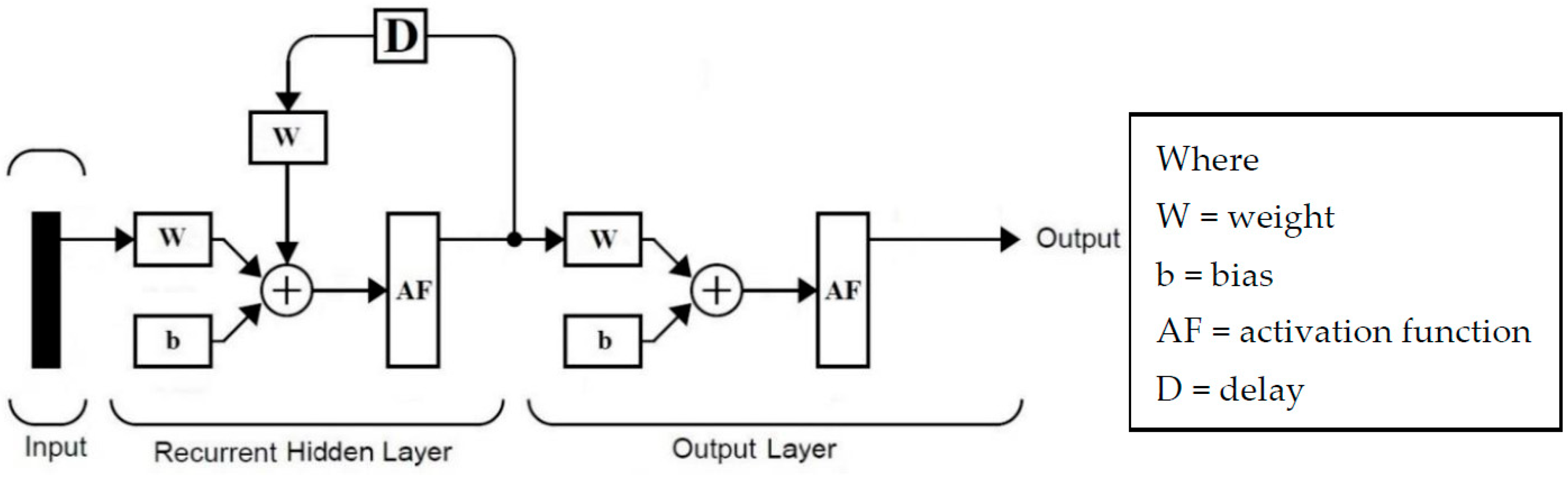
The output power estimation was performed for a NREL 5 MW WT using 2297 data samples. Four nonlinear parameters were selected as inputs due to their stochastic nature and included wind speed, rotor speed, pitch angle, and power coefficient of the WT. Results were collected through MATLAB simulations.

The PC used for this purpose was Intel^® Core™ i5-7200U CPU at 2.50 GHz (4 CPUs), ~2.7 GHz with 8 GB RAM, and Windows 10 Pro operating system. Each network was trained under five different conditions based on the number of hidden layers and activation functions assigned to each hidden layer, at four different learning rates; thus, generating twenty different results for each variant. The input layer in each case consisted of four nodes as four nonlinear parameters were used in the training, i.e., wind speed, angular speed of the rotor, blade pitch angle, and power coefficient of the WT. There were no weights, biases, or activation functions associated with this layer because the function of this layer was only to transfer input data to the hidden layers. The output layer in each case contains one node with a linear activation function.

The training conditions designed for the estimation were as follows:

• Case 1: The network consisted of two layers, i.e., one hidden layer with 100 nodes and a single-node output layer. The hidden layer was assigned a tan-sigmoid (tansig) activation function.
• Case 2: A three-layer network was designed with 100 nodes in the first hidden layer and 50 nodes in the second hidden layer. The activation functions assigned were tansig and logsig, respectively. The output layer contained a single purelin node.
• Case 3: The network consisted of a four-layer network. The first hidden layer contained 100 tansig nodes, the second hidden layer contained 50 logsig nodes, and the third hidden layer contained 25 tansig nodes. The output layer had a single purelin node.
• Case 4: This was similar to case 3 with one alteration, i.e., the second hidden layer was assigned with a tansig activation function, and the third hidden layer was assigned with a logsig function.
• Case 5: The designed network contained five layers with four hidden layers and an output layer. There were 100 nodes in the first hidden layer, 50 nodes in the second hidden layer, 25 nodes in the third hidden layer, and 12 nodes in the fourth hidden layer. The first and second hidden layers were assigned with a tansig activation function, and a logsig activation function was assigned to the third and fourth hidden layers. The above five cases are summarized in

  Table 3. Neural network configurations designed for each case.

  Layers	Nodes	Activation Functions
  		Case 1	Case2	Case 3	Case 4	Case 5
  Hidden Layer 1	100	tansig	tansig	tansig	tansig	tansig
  Hidden Layer 2	50	---	logsig	logsig	tansig	tansig
  Hidden Layer 3	25	---	---	tansig	logsig	logsig
  Hidden Layer 4	12	---	---	---	---	logsig
  Output Layer	1	purelin	purelin	purelin	purelin	purelin

  .

Each case was repeated at four different learning rates, i.e., 0.05, 0.03, 0.01, and 0.005. Thus, 20 results were recorded for each variant, yielding a total of 40 outcomes. Both networks were trained for 10,000 epochs under similar conditions and their performance was compared using MAPE and RMSE the primary testing factor and training time as the secondary factor. The target error was set to e⁻⁷ in each case, and the criterium for ending the training (learning) process was either the achievement of the target error or the completion of 10,000 epochs, whichever came first. Each network was trained using the SCG algorithm due to its smaller memory requirement. The Levenberg-Marquardt (LM) algorithm is faster than SCG, but it is only feasible for smaller data samples (i.e., about 100) and also requires more memory [50]. The Bayesian regularization (BR) algorithm is suitable for the small and noisy datasets and requires more training time.

Therefore, SCG was selected for this study. The MAPE and RMSE values were calculated while training the network, in each case to check the training performance of the respective network. After training the network with 70% data, a remaining 20% of the data was used to test the network performance, and the last 10% to validate and test of the calculated MAPE and RMSE values. The results recorded for each case are discussed below.

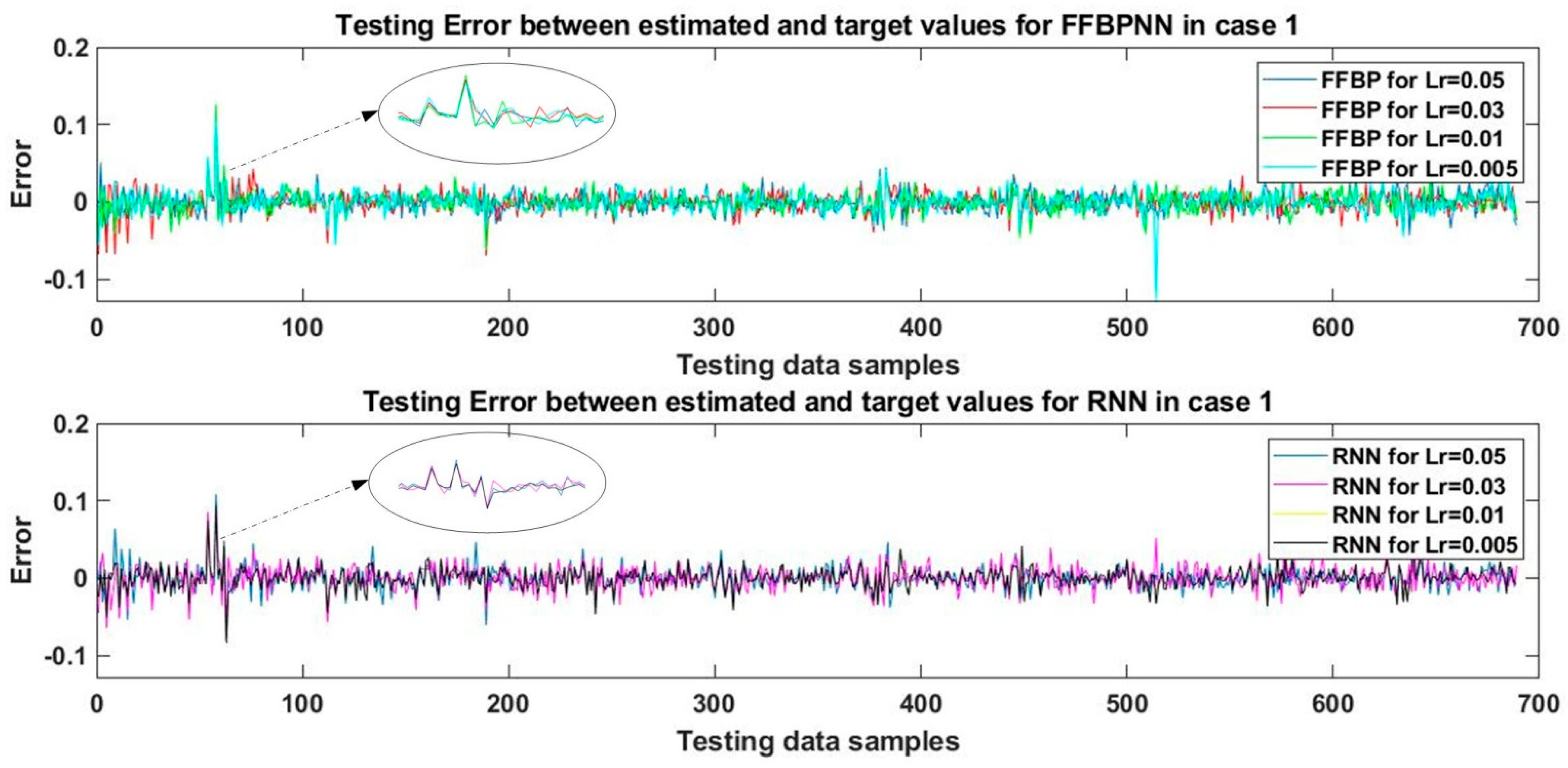
Case 1:

In the first case, a two-layered network was designed for FFBPNN and RNN with 100 tansig nodes in the hidden layer and one purelin node in the output layer. Both networks were trained at four learning rates, i.e., 0.05, 0.03, 0.01, and 0.005. The networks were trained with approximately 70% of the training data samples for 10,000 epochs, then tested with 20% of the testing data samples and validated using the remaining 10%.

The trained network was tested using the sim command in MATLAB to obtain the estimated values of WT output mechanical power. The estimated values were then compared to the actual values of output mechanical power in test data samples, and errors were plotted in Figure 4. The performance of the networks was verified by calculating the MAPE and RMSE for the estimated test data results-the results are shown in

Table 4. Training and testing results of FFBPNN and RNN for Case 1.

NN Variant	Learning Rate	Training Time	RMSE Testing	RMSE Validation	MAPE Testing	MAPE Validation
FFBP	0.05	46:17	0.0140	0.0129	0.12844	0.07556
	0.03	0:55	0.0145	0.0138	0.11141	0.07465
	0.01	0:53	0.0132	0.0116	0.07872	0.05921
	0.005	0:50	0.0136	0.0147	0.05595	0.08372
RNN	0.05	5:28	0.0156	0.0148	0.06694	0.06375
	0.03	1:49	0.0160	0.0147	0.08192	0.0574
	0.01	18:52	0.0135	0.0134	0.07125	0.09701
	0.005	24:12	0.0135	0.0134	0.07125	0.09701

. It can be seen that the test MAPE of 5.59% was the lowest in the case of FFBPNN for the learning rate of 0.005.

The RMSE of 1.32% was the lowest in the case of FFBPNN for the learning rate of 0.01. RNN showed the best performance with the MAPE score of 6.69% and the corresponding RMSE of 1.56%, for the learning rate of 0.05. With RMSE of 1.35%, RNN performed best for the learning rates of 0.01 and 0.005, but shorter training time is required for the learning rate of 0.01, which is why this learning rate was preferable. In terms of MAPE, the training time for the learning rate of 0.005 in the case of FFBPNN was also shorter, hence, this learning rate was selected for training.

It is evident that for a two-layered network trained with the SCG algorithm, the learning rate of 0.005 yielded the best performance for FFBPNN in terms of testing MAPE, while for RMSE, the learning rate of 0.01 returned the best performance for both FFBPNN and RNN, but FFBPNN performed better than RNN in terms of testing RMSE and training time. FFBPNN also outperformed RNN regarding training time. Hence, FFBPNN proved overall superior to RNN in this case.

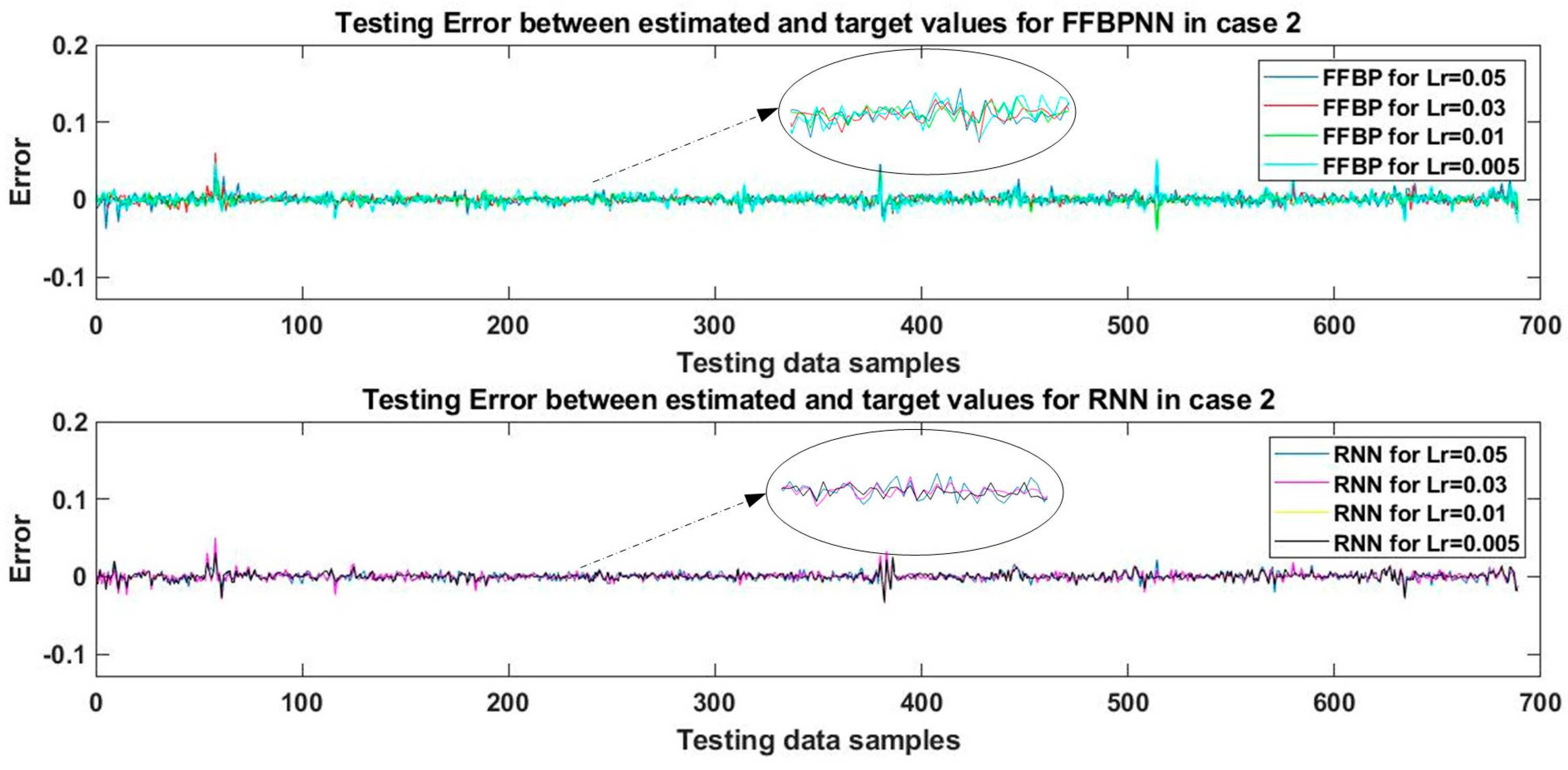
Case 2:

Three-layered FFBPNN and RNN models were designed for this case. Each network contained 100 tansig nodes and 50 logsig nodes in their first and second hidden layers, respectively. Both networks contained a single node in the output layer with a linear activation function. Both networks were trained with the SCG algorithm using training data samples for 10,000 epochs and the training process was repeated at four learning rates. The eight trained networks were then tested against the test data samples, validated, and the estimated values of WT mechanical output power were generated. The estimates were then compared to the target values of mechanical power, and the inconsistencies between estimated values and the target values are plotted in Figure 5. The performance estimate was verified by calculating the MAPE and RMSE between the estimated and target values of the test data, and the results are presented in

Table 5. Training and testing results of FFBPNN and RNN for case 2.

NN Variant	Learning Rate	Training Time	RMSE Testing	RMSE Validation	MAPE Testing	MAPE Validation
FFBP	0.05	1:34	0.0065	0.0062	0.02707	0.02267
	0.03	1:41	0.0056	0.0053	0.02198	0.02251
	0.01	18:50	0.0049	0.0051	0.02626	0.01986
	0.005	43:41	0.0071	0.0074	0.03041	0.01071
RNN	0.05	3:06	0.0059	0.0058	0.02105	0.02173
	0.03	2:56	0.0060	0.0058	0.0188	0.0243
	0.01	3:10	0.0052	0.0052	0.01737	0.01967
	0.005	25:41	0.0052	0.0052	0.01737	0.01967

.

It can be observed by comparing Table 4 and Table 5 that increasing a hidden layer in the network substantially improved the results, i.e., MAPE and RMSE values were significantly decreased. In the case of FFBPNN, the best result for testing data with the lowest RMSE of only 0.49% was recorded at learning rate of 0.01. In terms of MAPE, the best result for FFBPNN was achieved at the learning rate of 0.03, where MAPE was 2.19%. The RMSE of 0.49% for testing data was significantly lower than the lowest value of RMSE achieved in case 1, i.e., 1.32%recorded at the learning rate of 0.01 but the training time was increased in this case. MAPE also improved as compared to case 1 where it was 5.59% for the learning rate of 0.005. In the case of RNN, the best result was recorded for the learning rates of 0.01 and 0.005 where the value of RMSE was 0.52%.

For MAPE, RNN showed better result as compared to FFBPNN for the learning rates of 0.01 and 0.005, but the training time for the learning rate 0.01 is shorter, rendering this result better. It is very interesting to observe that for RNN, in case of the learning rates of 0.01 and 0.005, other test and validation parameters such as gradient, MAPE, and RMSE were similar, but the training time required at the learning rate of 0.005 was approximately eight times longer relative to the learning rate of 0.01.

This shows that the learning rate can significantly affect the training time of the network. Hence, the learning rate should be chosen wisely. In Figure 5, the yellow and black graphs representing the learning rates of 0.01 and 0.005 for RNN overlap completely, that is why the yellow graph is not visible. This verifies the data shown in Table 5. Consequently, in this case, FFBPNN showed better performance (for RMSE) than RNN, while RNN performed better in terms of MAPE.

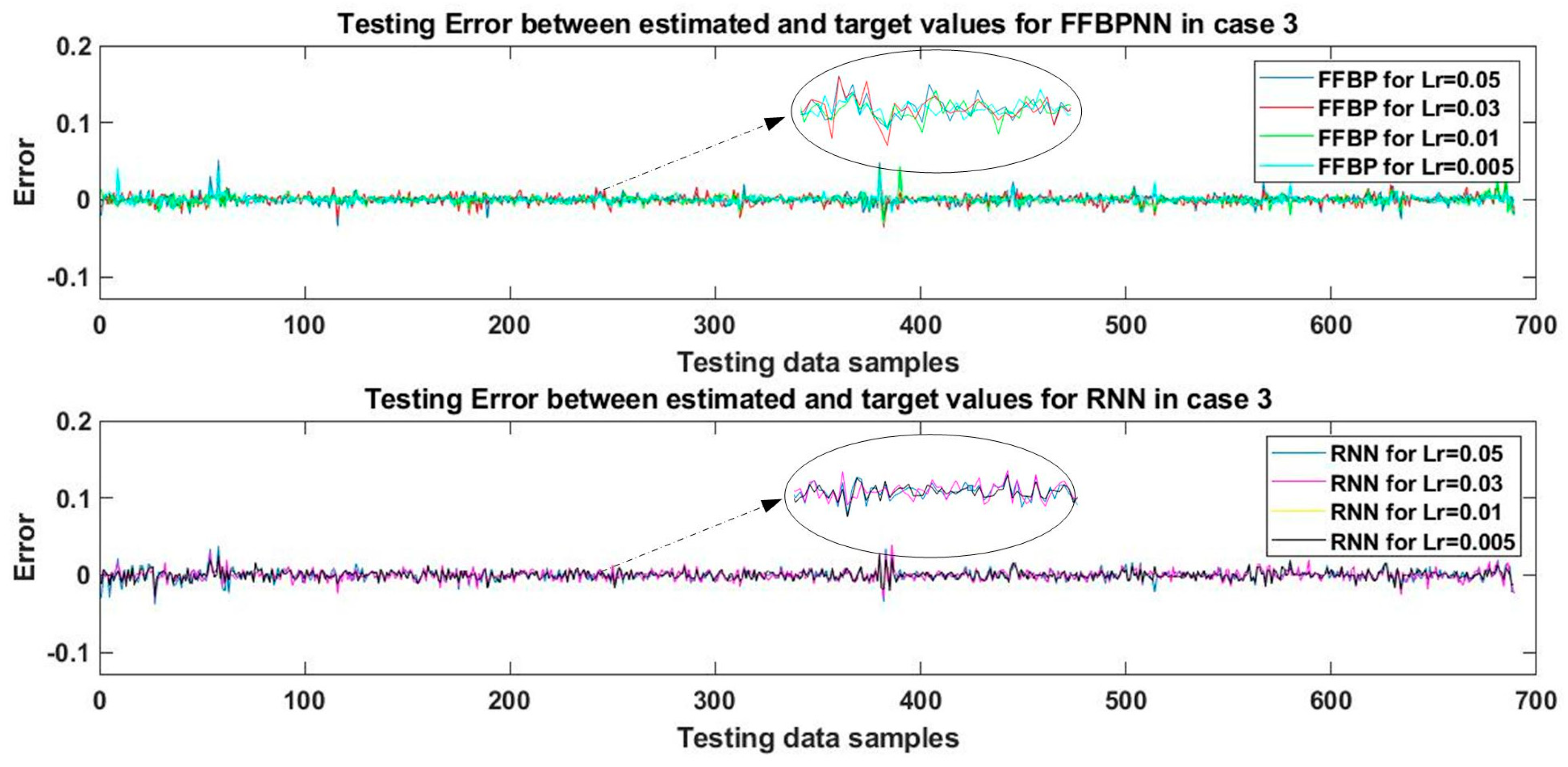
Case 3:

In this case, a new hidden layer with 25 nodes was added in both networks. Thus, each network consisted of four layers. The first, second, and third hidden layers contained 100, 50, and 25 nodes, respectively, and the activation functions assigned were tansig, logsig, and tansig, respectively. The output layer contained a single purelin node. The networks were trained with the SCG algorithm at four different learning rates and the training continues for 10,000 epochs.

After training, the networks were tested against the 465 test data samples and validated using the sim command in MATLAB to obtain the estimates. These estimations were then compared to the target values of the test data samples and the errors were plotted in a graph, as shown in Figure 6. The RMSE and MAPE of the test results were calculated and presented in

Table 6. Training and testing results of FFBPNN and RNN for case 3.

NN	Learning Rate	Training Time	RMSE Testing	RMSE Validation	MAPE Testing	MAPE Validation
FFBP	0.05	32:29	0.0069	0.0063	0.0307	0.0193
	0.03	5:24	0.0063	0.0062	0.0207	0.0191
	0.01	2:02	0.0057	0.005	0.01902	0.02215
	0.005	2:47	0.0055	0.0038	0.0194	0.01223
RNN	0.05	4:32	0.0075	0.0078	0.0285	0.0335
	0.03	3:27	0.0069	0.0063	0.0218	0.0203
	0.01	3:20	0.0059	0.0057	0.0243	0.0325
	0.005	20:00	0.0059	0.0057	0.0243	0.0325

.

In the case of FFBPNN, the best result was obtained for the learning rate of 0.005 with the RMSE of 0.55%. The best result for MAPE, i.e., 1.9%, was recorded for the learning rate of 0.01. For RNN, the best performance was achieved at the learning rates of 0.01 and 0.005, where RMSE was 0.59%, and MAPE was 2.18%, achieved for the learning rate of 0.01. Again, it can be observed that in the case of RNN, the network’s behavior was similar to case 2. In both instances, at the learning rates of 0.01 and 0.005, the values of gradient, testing, and validation results for RMSE and MAPE were the same.

For the learning rate of 0.005, approximately six times more training time was required with no improvement in performance. Those data can also be verified against Figure 6, where the yellow graph for the RNN learning rate 0.01 and the black graph for the RNN learning rate 0.005 overlap completely. Therefore, the yellow graph is not visible in Figure 6. The learning rate of 0.01 appears to have been the best choice for both FFBPNN and RNN in the case of MAPE. From these results, it can be concluded that FFBPNN performed better in this case in terms of both MAPE and RMSE.

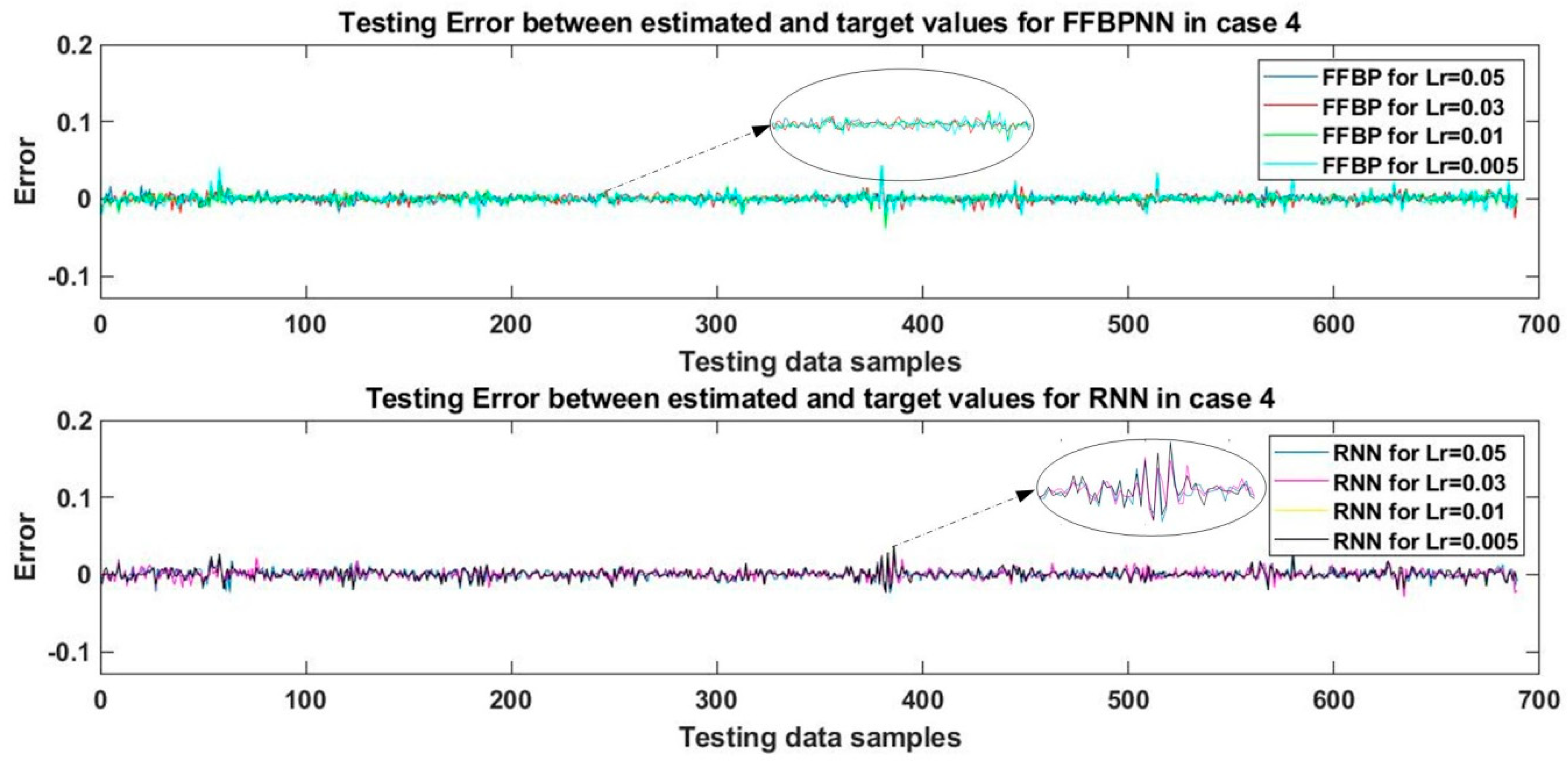
Case 4:

The networks designed in this case contained four layers each. The first and second hidden layers contained 100 and 50 tansig nodes, respectively. The third hidden layer contained 25 nodes with a log-sigmoid activation function, and the fourth layer was the output layer with a single purelin node. The networks were trained using the SCG algorithm for 10,000 epochs at the four learning rates mentioned above.

After training, the networks’ performance was tested and validated, and the estimated WT mechanical output power was calculated. The results were then compared to the actual values of WT mechanical output power from the test data samples, and the errors were plotted in the graph shown in Figure 7. The value of RMSE relative to the estimated and actual values of WT mechanical output power was calculated for every tested network and the results are presented in

Table 7. Training and testing results of FFBPNN and RNN for case 4.

NN Variant	Learning Rate	Training Time	RMSE Testing	RMSE Validation	MAPE Testing	MAPE Validation
FFBP	0.05	15:15	0.0050	0.0045	0.0216	0.0212
	0.03	2:05	0.0051	0.0051	0.0215	0.0226
	0.01	1:58	0.0050	0.0051	0.0133	0.0211
	0.005	2:05	0.0062	0.00058	0.0237	0.0241
RNN	0.05	30:12	0.0065	0.0064	0.0365	0.0361
	0.03	3:27	0.0060	0.0062	0.0269	0.0287
	0.01	3:20	0.0063	0.0057	0.0337	0.0286
	0.005	3:48	0.0063	0.0057	0.0337	0.0286

.

The results displayed in Table 6 and Table 7 are for networks with a similar number of hidden layers, the same number of nodes in each layer, and trained with the same algorithm for an equal number of epochs. There was only one difference between these two cases, i.e., the assigned activation functions. Specifically, the activation functions for the second and third hidden layers in the respective cases were swapped. By comparing the data in Table 6 and Table 7, it can be observed that the results improved in case 4 for both FFBPNN and RNN. This shows the importance of assigning activation functions to each layer of the network. In the case of FFBPNN, the best performance was achieved at the learning rates of 0.05 and 0.01 where the value of RMSE was 0.5%. Of the two, the training time for the learning rate of 0.01 is lower, hence was preferable. The best value of MAPE (1.33%) was also achieved for the learning rate of 0.01. In the case of RNN, the best performance with RMSE of 0.6% and MAPE of 2.69% was recorded for the learning rate of 0.03. Once again, a repetition of RNN results for the learning rates of 0.01 and 0.005 was observed. This behavior was also verified with the graph shown in Figure 7, where the yellow and black graphs representing the learning rates of 0.01 and 0.005, respectively, overlap in the case of RNN, hence rendering the yellow graph invisible. This behavior shows that for cases 2, 3, and 4, decreasing the learning rate does not affect the output of the RNN network. Overall, FFBPNN outperformed RNN in this case.

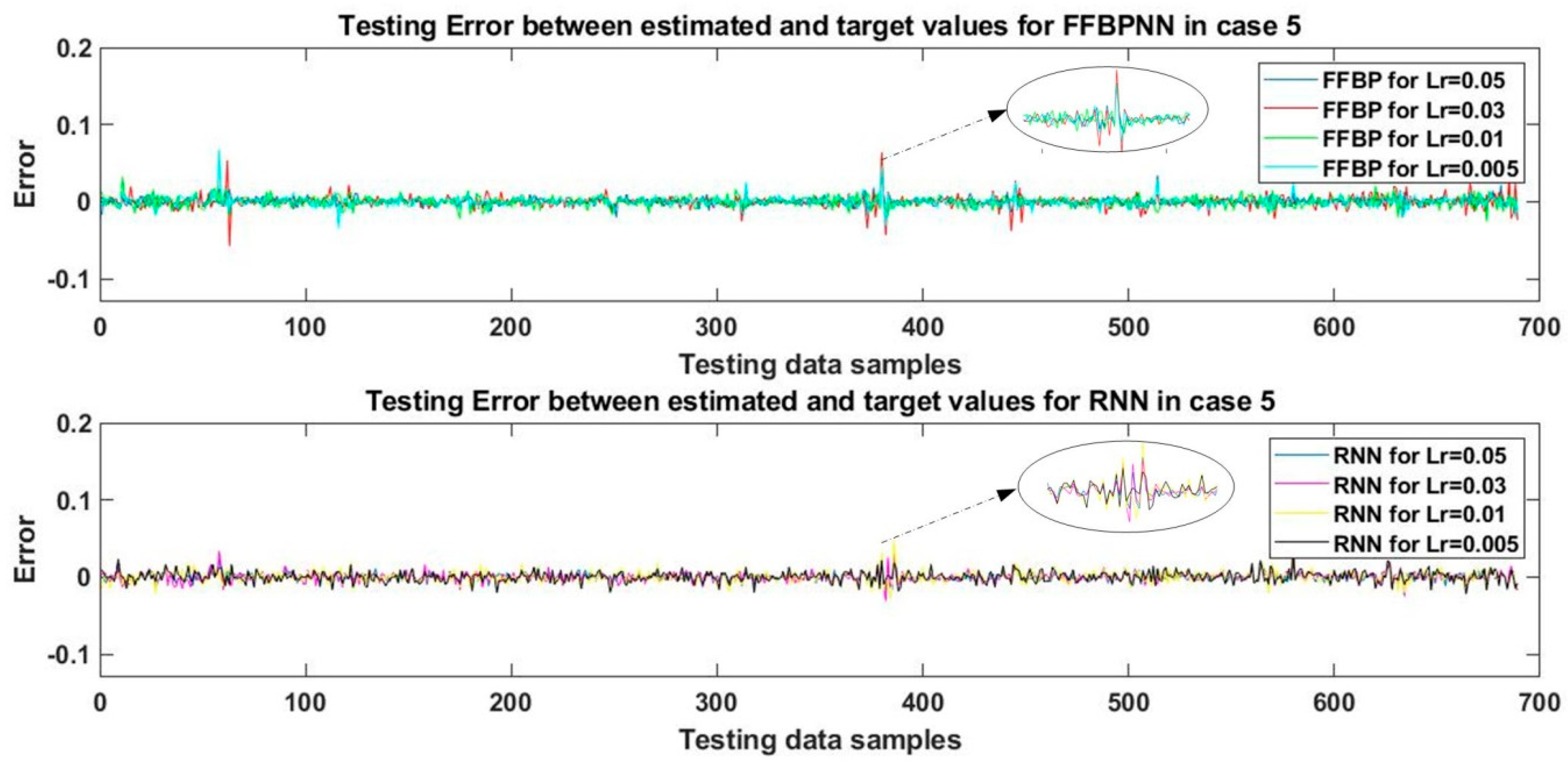
Case 5:

In the final case, five-layered networks were designed for FFBPNN and RNN. The first and second hidden layers contained 100 and 50 nodes, respectively, with a tan-sigmoid activation function, and the third and fourth hidden layers contained 25 and 12 nodes, respectively, with a log-sigmoid activation function. The fifth layer was the output layer with a single purelin node. The training process in both networks was repeated at four learning rates. The networks were trained using the SCG algorithm and the performance of every trained network was tested and validated to obtain the estimated value of WT output mechanical power. This estimated result was then compared to the actual values of mechanical power and the errors were plotted in the graph shown in Figure 8. The performance of the networks was evaluated by calculating RMSE and MAPE in each case. The training and testing results are shown in

Table 8. Training and testing results of FFBPNN and RNN for case 5.

NN Variant	Learning Rate	Training Time	RMSE Testing	RMSE Validation	MAPE Testing	MAPE Validation
FFBP	0.05	1:20:56	0.0056	0.0059	0.0213	0.0185
	0.03	4:23	0.0079	0.0084	0.0181	0.0157
	0.01	1:35:10	0.0069	0.0066	0.0331	0.0303
	0.005	2:06	0.0062	0.0056	0.0227	0.0175
RNN	0.05	4:07	0.0055	0.0051	0.0286	0.0257
	0.03	3:49	0.0062	0.0059	0.0331	0.05
	0.01	4:39	0.0074	0.0068	0.0435	0.0311
	0.005	41:23	0.0070	0.0067	0.0418	0.0266

.

In the case of FFBPNN, the best performance was achieved for the learning rate of 0.05 where the value of RMSE was 0.56%. The best result for MAPE was 1.81% recorded at the learning rate of 0.03. The second-best performance, in this case, was observed for the learning rate of 0.005 with the RMSE value of 0.62%. Although there was a 0.06% performance discrepancy, the corresponding difference in training time was quite substantial. The training time for the learning rate of 0.05 was forty times longer than that in the case of 0.005.

Thus, in this case, a 0.06% error can be absorbed if training time is a critical factor. to the ultimate choice will depend on the priorities applicable to the given practical situation. In the case of RNN, the best performance with the lowest value of RMSE (0.55%) was achieved for the learning rate of 0.05. This was the only case where RNN actually outperformed FFBPNN by 0.01%, with a training time for the learning rate of 0.05 approximately twenty times shorter compared to FFBPNN. In terms of MAPE, RNN yielded the best result for the learning rate of 0.05, with MAPE at the level of 2.86%, which was higher than the 1.81% observed in case of FFBPNN.

As follows from the above discussion, FFBPNN performed better in the first four cases, while RNN yielded better results only in the last case, with a 0.01% improvement in RMSE value. As for MAPE, FFBPNN also performed better in four out of the five cases.

Table 9. Training and testing results of FFBPNN and RNN for all cases.

NN Variant	Cases	Training Time	Gradient	RMSE Testing	RMSE Validation	MAPE Testing	MAPE Validation
FFBP with Lr = 0.05	Case 1	46:17	0.00211	0.0140	0.0129	0.12844	0.07556
	Case 2	1:34	0.00109	0.0065	0.0062	0.02707	0.02267
	Case 3	32:29	0.00111	0.0069	0.0063	0.0307	0.0193
	Case 4	15:15	0.00235	0.0050	0.0045	0.0216	0.0212
	Case 5	1:20:56	0.00194	0.0056	0.0059	0.0213	0.0185
FFBP with Lr = 0.03	Case 1	0:55	0.00230	0.0145	0.0138	0.11141	0.07465
	Case 2	1:41	0.00204	0.0056	0.0053	0.02198	0.02251
	Case 3	5:24	0.00274	0.0063	0.0062	0.0207	0.0191
	Case 4	2:05	0.00149	0.0051	0.0051	0.0215	0.0226
	Case 5	4:23	0.00167	0.0079	0.0084	0.0181	0.0157
FFBP with Lr = 0.01	Case 1	0:53	0.00145	0.0132	0.0116	0.07872	0.05921
	Case 2	18:50	0.00116	0.0049	0.0051	0.02626	0.01986
	Case 3	2:02	0.00148	0.0057	0.005	0.01902	0.02215
	Case 4	1:58	0.00177	0.0050	0.0051	0.0133	0.0211
	Case 5	1:35:10	0.00537	0.0069	0.0066	0.0331	0.0303
FFBP with Lr = 0.005	Case 1	0:50	0.00124	0.0136	0.0147	0.05595	0.08372
	Case 2	43:41	0.00100	0.0071	0.0074	0.03041	0.01071
	Case 3	2:47	0.00126	0.0055	0.0038	0.0194	0.01223
	Case 4	2:05	0.000922	0.0062	0.00058	0.0237	0.0241
	Case 5	2:06	0.000989	0.0062	0.0056	0.0227	0.0175
RNN with Lr = 0.05	Case 1	5:28	0.00789	0.0156	0.0148	0.06694	0.06375
	Case 2	3:06	0.000558	0.0059	0.0058	0.02105	0.02173
	Case 3	4:32	0.00297	0.0075	0.0078	0.0285	0.0335
	Case 4	30:12	0.00308	0.0065	0.0064	0.0365	0.0361
	Case 5	4:07	0.00384	0.0055	0.0051	0.0286	0.0257
RNN with Lr = 0.03	Case 1	1:49	0.0114	0.0160	0.0147	0.08192	0.0574
	Case 2	2:56	0.00092	0.0060	0.0058	0.0188	0.0243
	Case 3	3:27	0.00399	0.0069	0.0063	0.0218	0.0203
	Case 4	3:27	0.00231	0.0060	0.0062	0.0269	0.0286
	Case 5	3:49	0.00704	0.0062	0.0059	0.0331	0.050
RNN with Lr = 0.01	Case 1	18:52	0.004707	0.0135	0.0134	0.07125	0.09701
	Case 2	3:10	0.00269	0.0052	0.0052	0.01737	0.01967
	Case 3	3:20	0.000626	0.0059	0.0057	0.0243	0.0325
	Case 4	3:20	0.00174	0.0063	0.0057	0.0337	0.0286
	Case 5	4:39	0.00354	0.0074	0.0068	0.0435	0.0311
RNN with Lr = 0.005	Case 1	24:12	0.004707	0.0135	0.0134	0.07125	0.09701
	Case 2	25:41	0.00269	0.0052	0.0052	0.01737	0.01967
	Case 3	20:00	0.000626	0.0059	0.0057	0.0243	0.0325
	Case 4	3:48	0.00174	0.0063	0.0057	0.0337	0.0286
	Case 5	41:23	0.0126	0.0070	0.0067	0.0418	0.0266

summarizes all the results sorted by the learning rate. It must be noted that the performance of different NNs depends upon the complexity of the dataset, so these results can only be generalized for cases where there are four input parameters and a single output variable. Based on the above, it can be concluded that the performance of the NNs depended on various factors that include several hidden layers, assigned activation functions, and different values of learning rates. The number of nodes assigned to each layer also affected the performance, but this aspect was not considered in this study and will be elaborated in future research.

Five different cases were examined with a view to finding the best estimation achievable using two different NN variants, i.e., FFBPNN and RNN. The effect of changing the number of hidden layers was best observed in case 1 and case 2 where the network performance in the second case improved by over 50%. In the subsequent cases, the performance of the networks was not significantly affected by further increasing the number of hidden layers. This shows that if networks are modeled under similar conditions, better performance can be achieved using two hidden layers.

The importance of assigning a suitable activation function can be observed in cases 3 and 4, where the second and third hidden layers were assigned with log-sigmoid and tan-sigmoid activation functions for FFBPNN, and tan-sigmoid and log-sigmoid activation functions for RNN, respectively. The tan-sigmoid activation function limits its output range to −1–1, while the log-sigmoid activation function gives the output in the range from 0 to 1. Therefore, these activation functions are not assigned to the output layer if the required output value lies outside said ranges. For that reason, the output node in every case considered in this study was assigned with a linear activation function to allow for outputs outside the range of −1 and 1. By swapping the activation functions for the second and third hidden layers in case 3 and case 4, respectively, the results of FFBPNN improved at the learning rates of 0.05, 0.03, and 0.01, while the learning rate of 0.005 yielded worse result in case 4. For RNN, the learning rates of 0.05 and 0.03 showed improved performance in case 4, while the learning rates of 0.01 and 0.005 showed better performance in case 3. The value of the learning rate controls the rate of the network’s adaptation to the given problem. Generally, this value lies between 0 and 1. Four different values of learning rates were used in this study, namely 0.05, 0.03, 0.01, and 0.005. However, the changing learning rates had a random impact on performance. In the case of FFBPNN, the performance of the network was random for the first case. In the second case, the network performance improved with the learning rates (Lr) decreasing from 0.05 to 0.01, but further decrease deteriorated the network performance.

In case 3, the network performance improved with the learning rates decreasing from 0.05 to 0.005. Case 4 has showed the most promising results for the learning rates from 0.05 to 0.01 where the value of RMSE ranges from 0.5% to 0.51%.

However, further decrease of the learning rate had a negative impact on network performance. In the fifth case, the best performance was observed for the learning rate of 0.05, but decreasing the value of the learning rate to 0.03 drastically degraded the network performance. Further decrease of the learning rates somewhat improved the network performance but never reaching the level recorded for the learning rate of 0.05. In the case of RNN, the network performed randomly for the learning rates of 0.05 and 0.03. However, it must be noted that in the first four cases, the networks showed similar behavior when the learning rate was decreased from 0.01 to 0.005. In the fifth case, the testing results deteriorated for learning rates from 0.05 to 0.01. A further decrease in the learning rate showed some improvement in the quality of estimations results but not enough to outdo the result achieved at the learning rate of 0.05.

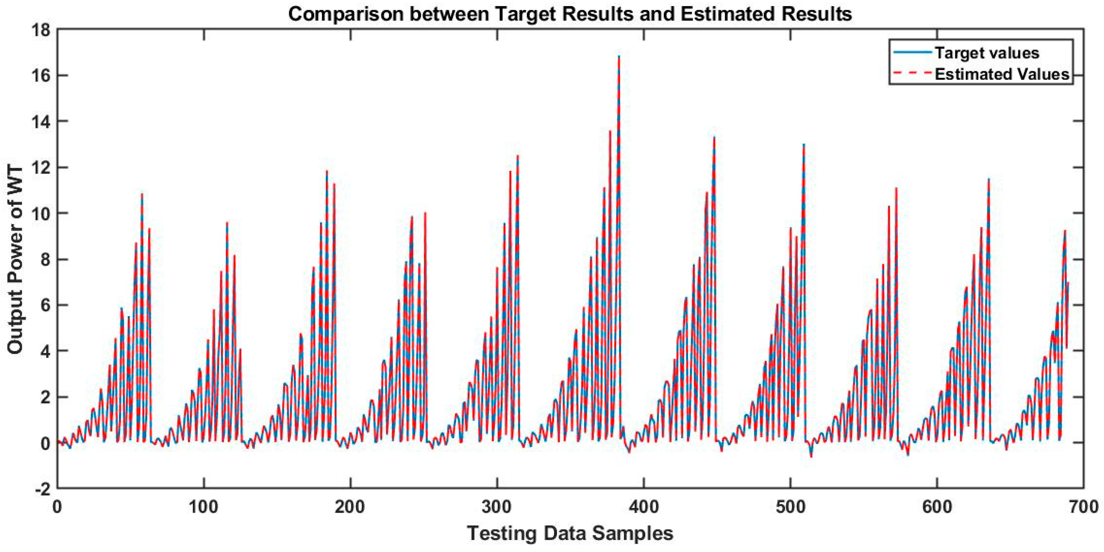
Consequently, it can be concluded that RNN will not improve performance if the learning rate is decreased beyond 0.01, provided that the network is designed for a similar problem. In terms of FFBPNN, the best overall result was observed for the learning rate of 0.01 using case 2 with two hidden layers comprising 100 tansig and 50 logsig nodes in first and second hidden layers, respectively, where the value of RMSE was 0.49%. As for MAPE, FFBPNN once again outperformed the alternative showing the best results in case 4 with three hidden layers. A graph comparing the target and estimated values is provided in Figure 9. It shows that the estimated results were very close to the actual target values.

The second-best result was achieved for the same value of learning rate using case 4 with three hidden layers comprising 100 and 50 tansig nodes in the first and second hidden layers, and 25 logsig nodes in the third hidden layer, where the value of RMSE was 0.5%. However, the training time for case 4 was approximately nine times shorter than in case 2. Therefore, deepening on the priority applicable to a given situation, one can choose between methods yielding the lowest values of RMSE, MAPE, or the shortest training time. Notably, however, training time can be also improved if GPUs are used instead of CPUs.

For comparison purposes, an advanced variant of RNN was also used, i.e., long short-term memory (LSTM), for the estimations in all five cases, and the average test errors are summarized in

Table 10. Testing results of FFBPNN, RNN, and LSTM for all cases.

NN Variant	FFBPNN		RNN		LSTM
Avg. Error	RMSE	MAPE	RMSE	MAPE	RMSE	MAPE
Case 1	0.01382	0.09363	0.01465	0.07284	0.3634515	118.2736
Case 2	0.00512	0.02643	0.00558	0.01865	0.3917926	805.1603
Case 3	0.00610	0.02246	0.00655	0.02472	0.3930577	126.0075
Case 4	0.00532	0.02002	0.00628	0.03270	0.3965067	124.8224
Case 5	0.00665	0.02380	0.00652	0.03675	0.3971354	129.4237

. The training times of LSTM for all five cases are recorded as 17:69, 20:28, 23:74, 29:69, and 32:34 s. The best LSTM result was recorded for case 1, where RMSE was 0.36345 and MAPE was 118.273, i.e., considerably worse than the results of either FFBPNN or RNN. As follows from the juxtaposition, FFBPNN overall outperformed both RNN and LSTM.

5. Conclusions

In this study, the mechanical output power of a WT was estimated using two variants of NNs, namely FFBPNN and RNN. The soft computing techniques were chosen due to their robustness and ability to develop non-linear relationships between stochastic input and output variables. The input parameters used for this study included wind speed, rotor speed, collective blade pitch angle, and WT power coefficient. Two variants of NNs are then designed for five different cases based on several hidden layers, activation functions assigned to each layer, and learning rates. For each case, both networks were trained using the SCG algorithm at four different learning rates using training data, after which the trained networks were used to estimate the output mechanical power of a WT based on the testing data. Subsequently, the results were successfully validated. The best results were achieved with the use of FFBPNN in case 2 where the value of RMSE was 0.49%, and in case 4 when MAPE was 1.33%. The second-best result was obtained for the same learning rate in case 4—yielding RMSE of 0.5%. RNN produced the best estimation in case 2 with MAPE of 1.73%, and in case 2 where RMSE was 0.52%. The present paper explored the effects of changing several hidden layers, assigning different activation functions, and changing learning rates on the performance of these variants of NNs. Notably, this methodology also reduces the need for sensors measuring atmospheric parameters such as air density, temperature, humidity, etc. The models can be easily implemented using interfacing cards such as dSPACE and NI cards. However, the main disadvantage of this methodology is its dependence on detailed WT parameter data that were used here as inputs in the estimations, as sometimes such parameters are not documented in sufficient detail over long periods of time.

In future research, the estimated mechanical output power of a WT can be used to determine the electrical power output of the WT. Further research on these models may explore the effect of changing several nodes in each hidden layer and further changing the activation functions. The models may be also used to further investigate other parameters of WTs such as TSR, C_P, or optimal rotor speed using MPPT. The future research may also include the estimation of noise level in wind turbines and the study of wake effect in off-shore and on-shore wind farms. Furthermore, the results may be compared using other advanced and more complex soft computing techniques, e.g., GRU and ANFIS, or other hybrid NN techniques.

References

1. Elavarasan, R.M. The Motivation for Renewable Energy and its Comparison with Other Energy Sources: A Review. Eur. J. Sustain. Dev. Res. 2019, 3, em0076. [Google Scholar] [CrossRef]
2. Frazier, A.W.; Marcy, C.; Cole, W. Wind and solar PV deployment after tax credits expire: A view from the standard scenarios and the annual energy outlook. Electr. J. 2019, 32, 106637. [Google Scholar] [CrossRef]
3. REN21. “Renewable Energy Policy Network for 21st Century,” Renewables 2019 Global Status Report. Available online: http://www.ren21.net/gsr-2019/ (accessed on 3 April 2019).
4. Solyali, D.; Altunç, M.; Tolun, S.; Aslan, Z. Wind resource assessment of Northern Cyprus. Renew. Sustain. Energy Rev. 2016, 55, 180–187. [Google Scholar] [CrossRef]
5. Peng, X.; Xiong, L.; Wen, J.; Cheng, S.; Deng, D.; Feng, S.; Wang, B. A summary of improved methods for short-term and ultra-short-term power forecasting accuracy of wind power clusters. Procedings CSEE 2016, 36, 6315–6326. [Google Scholar]
6. Jung, J.; Broadwater, R.P. Current status and advances for wind speed and power forecasting. Renew. Sustain. Energy Rev. 2014, 31, 762–777. [Google Scholar] [CrossRef]
7. Qian, Z.; Pei, Y.; Cao, L.; Wang, J.; Jing, B. Review of wind power forecasting methods. High Volt. Technol. 2016, 42, 1047–1060. [Google Scholar]
8. Foley, A.M.; Leahy, P.G.; Marvuglia, A.; McKeogh, E.J. Current methods and advances in forecasting of wind power generation. Renew. Energy 2012, 37, 1–8. [Google Scholar] [CrossRef] [Green Version]
9. Zhang, J.; Yan, J.; Infield, D.; Liu, Y.; Lien, F.-S. Short-term forecasting and uncertainty analysis of wind turbine power based on long short-term memory network and Gaussian mixture model. Appl. Energy 2019, 241, 229–244. [Google Scholar] [CrossRef] [Green Version]
10. Olaofe, Z.O.; Folly, K.A. Wind power estimation using recurrent neural network technique. In Proceedings of the IEEE Power and Energy Society Conference and Exposition in Africa: Intelligent Grid Integration of Renewable Energy Resources (PowerAfrica), Johannesburg, South Africa, 9–13 July 2012; pp. 1–7. [Google Scholar]
11. Munteanu, I.; Besançon, G. Prediction of wind park output power based on turbine effective wind speed—A model iden-tification approach. In Proceedings of the 2014 IEEE International Energy Conference (ENERGYCON), Cavtat, Republika Hrvatska, 13–16 May 2014; pp. 451–458. [Google Scholar]
12. Hayashi, M.; Nagasaka, K. Wind speed prediction and determination of wind power output with multi-area weather data by deterministic chaos. In Proceedings of the 2014 International Conference on Advanced Mechatronic Systems, Kumamoto, Japan, 10–12 August 2014; pp. 192–197. [Google Scholar]
13. He, M.; Vittal, V.; Zhang, J. A sparsified vector autoregressive model for short-term wind farm power forecasting. In Proceedings of the 2015 IEEE Power & Energy Society General Meeting, Denver, CO, USA, 26–30 July 2015; pp. 1–5. [Google Scholar]
14. Zolfaghari, S.; Riahy, G.H.; Abedi, M. A new method to adequate assessment of wind farms’ power output. Energy Convers. Manag. 2015, 103, 585–604. [Google Scholar] [CrossRef]
15. Hu, S.; Li, K.-J. Short-Term Wind Power Prediction Based on Principal Component Analysis and Elman Artificial Neural Networks. In Proceedings of the 2017 4th International Conference on Information Science and Control Engineering (ICISCE), Changsha, China, 21–23 July 2017; pp. 673–677. [Google Scholar]
16. Ba, M.M.; Ramenah, H.; Tanougast, C.; Madani, M. Power energy output prediction of small wind urban for decision making. In Proceedings of the 2017 4th International Conference on Control, Decision and Information Technologies (CoDIT), Barcelona, Spain, 5–7 April 2017; pp. 1102–1106. [Google Scholar]
17. Marčiukaitis, M.; Žutautaitė, I.; Martišauskas, L.; Jokšas, B.; Gecevičius, G.; Sfetsos, A. Non-linear regression model for wind turbine power curve. Renew. Energy 2017, 113, 732–741. [Google Scholar] [CrossRef]
18. Chang, G.; Lu, H.; Chang, Y.; Lee, Y. An improved neural network-based approach for short-term wind speed and power forecast. Renew. Energy 2017, 105, 301–311. [Google Scholar] [CrossRef]
19. Asghar, A.B.; Liu, X. Estimation of wind turbine power coefficient by adaptive neuro-fuzzy methodology. Neurocomputing 2017, 238, 227–233. [Google Scholar] [CrossRef]
20. Asghar, A.B.; Liu, X. Adaptive neuro-fuzzy algorithm to estimate effective wind speed and optimal rotor speed for var-iable-speed wind turbine. Neurocomputing 2018, 272, 495–504. [Google Scholar] [CrossRef]
21. Asghar, A.B.; Liu, X. Online Estimation of Wind Turbine Tip Speed Ratio by Adaptive Neuro-Fuzzy Algorithm. Int. J. Adv. Comput. Sci. Appl. 2018, 9, 28–33. [Google Scholar]
22. Shezan, S.; Julai, S.; Kibria, M.; Ullah, K.; Saidur, R.; Chong, W.; Akikur, R. Performance analysis of an off-grid wind-PV (photovoltaic)-diesel-battery hybrid energy system feasible for remote areas. J. Clean. Prod. 2016, 125, 121–132. [Google Scholar] [CrossRef]
23. Kulunk, E. Aerodynamics of Wind Turbines, Fundamental and Advanced Topics in Wind Power; Carriveau, R., Ed.; InTech: Rijeka, Croatia, 2011; ISBN 978-953-307-508-2. [Google Scholar]
24. Energy.Gov. Wind Energy Technologies Office. 2019. Available online: http://www.wind.energy.gov (accessed on 10 April 2019).
25. Polinder, H.; de Haan, S.W.H.; Dubois, M.; Slootweg, J.G. Basic Operation Principles and Electrical Conversion Systems of Wind Turbines. EPE J. 2005, 15, 43–50. [Google Scholar] [CrossRef]
26. Matayoshi, H.; Howlader, A.M.; Datta, M.; Senjyu, T. Control strategy of PMSG based wind energy conversion system under strong wind conditions. Energy Sustain. Dev. 2018, 45, 211–218. [Google Scholar] [CrossRef]
27. Asghar, A.B.; Liu, X. Estimation of wind speed probability distribution and wind energy potential using adaptive neuro-fuzzy methodology. Neurocomputing 2018, 287, 58–67. [Google Scholar] [CrossRef]
28. Jonkman, J.; Butterfield, S.; Musial, W.; Scott, G. Definition of a 5-MW Reference Wind Turbine for Offshore System Development; National Renewable Energy Laboratory: Golden, CO, USA, 2009.
29. Martin, H.R.; Kimball, R.W.; Viselli, A.M.; Goupee, A.J. Methodology for Wind/Wave Basin Testing of Floating Offshore Wind Turbines. Offshore Mech. Arct. Eng. 2014, 136, 020905. [Google Scholar] [CrossRef]
30. Koo, B.J.; Goupee, A.J.; Kimball, R.W.; Lambrakos, K.F. Model Tests for a Floating Wind Turbine on Three Different Floaters. Offshore Mech. Arct. Eng. 2014, 136, 020907. [Google Scholar] [CrossRef]
31. Vijayakumar, G.; Lavely, A.W.; Jayaraman, B.; Craven, B.; Brasseur, J. Blade Boundary Layer Response to Atmospheric Boundary Layer Turbulence on a NREL 5MW Wind Turbine Blade with Hybrid URANS-LES; American Institute of Aeronautics and Astronautics: Reston, VA, USA, 2014. [Google Scholar]
32. de Ridder, E.; Otto, W.; Zondervan, G.; Huijs, F.; Vaz, G. Development of a Scaled-Down Floating Wind Turbine for Offshore Basin Testing. In Proceedings of the ASME 2014 33rd International Conference on Ocean, Offshore and Arctic Engineering, San Francisco, CA, USA, 8 June 2014; Volume 9A. [Google Scholar]
33. Siddiqui, M.S.; Rasheed, A.; Tabib, M.; Kvamsdal, T. Numerical Analysis of NREL 5MW Wind Turbine: A Study Towards a Better Understanding of Wake Characteristic and Torque Generation Mechanism. J. Phys. Conf. Ser. 2016, 753, 32059. [Google Scholar] [CrossRef] [Green Version]
34. Nejad, A.R.; Guo, Y.; Gao, Z.; Moan, T. Development of a 5 MW reference gearbox for offshore. Wind Energy 2016, 19, 1089–1106. [Google Scholar] [CrossRef] [Green Version]
35. Hsu, M.; Akkerman, I.; Bazilevs, Y. Finite element simulation of wind turbine aerodynamics: Validation study using NREL Phase VI experiment ABSTRACT. Wind Energy 2014, 17, 461–481. [Google Scholar] [CrossRef]
36. Lago, L.I.; Ponta, F.L.; Otero, A.D. Analysis of alternative adaptive geometrical configurations for the NREL-5 MW wind turbine blade. Renew. Energy 2013, 59, 13–22. [Google Scholar] [CrossRef]
37. Jain, T.; Yamé, J.; Sauter, D. A Novel Approach to Real-Time Fault Accommodation in NREL’s 5-MW Wind Turbine Systems. IEEE Trans. Sustain. Energy 2013, 4, 1082–1090. [Google Scholar] [CrossRef]
38. Bazilevs, Y.; Hsu, M.-C.; Takizawa, K.; Tezduyar, T. Ale-vms and st-vms methods for computer modeling of wind-turbine rotor aerodynamics and fluid–structure interaction. Math. Model. Methods Appl. Sci. 2012, 22, 1230002. [Google Scholar] [CrossRef]
39. Sebastian, T.; Lackner, M. Characterization of the unsteady aerodynamics of offshore floating wind turbines. Wind Energy 2012, 16, 339–352. [Google Scholar] [CrossRef]
40. Ormberg, H.; Bachynski, E.E. Global Analysis of Floating Wind Turbines: Code Development, Model Sensitivity and Benchmark Study. In Proceedings of the Twenty-second (2012) International Offshore and Polar Engineering Conference, Rhodes, Greece, 17–22 June 2012; Volume 4, pp. 366–373. [Google Scholar]
41. Hsu, M.-C.; Bazilevs, Y. Fluid–structure interaction modeling of wind turbines: Simulating the full machine. Comput. Mech. 2012, 50, 821–833. [Google Scholar] [CrossRef]
42. Lefebvre, S.; Collu, M. Preliminary design of a floating support structure for a 5MW offshore wind turbine. Ocean Eng. 2012, 40, 15–26. [Google Scholar] [CrossRef]
43. Hsu, M.-C.; Akkerman, I.; Bazilevs, Y. Wind turbine aerodynamics using ALE–VMS: Validation and the role of weakly enforced boundary conditions. Comput. Mech. 2012, 50, 499–511. [Google Scholar] [CrossRef]
44. Homola, M.C.; Virk, M.S.; Nicklasson, P.J.; Sundsbø, P.A. Performance losses due to ice accretion for a 5 MW wind turbine. Wind Energy 2011, 15, 379–389. [Google Scholar] [CrossRef]
45. Zhao, Y.; Yang, J.; He, Y. Preliminary Design of a Multi-Column TLP Foundation for a 5-MW Offshore Wind Turbine. Energies 2012, 5, 3874–3891. [Google Scholar] [CrossRef]
46. Nutakor, C.; Kłodowski, A.; Sopanen, J.; Mikkola, A.; Pedrero, J.I. Planetary gear sets power loss modeling: Application to wind turbines. Tribol. Int. 2017, 105, 42–54. [Google Scholar] [CrossRef]
47. Liu, J.; Xu, Z. A simulation investigation of lubricating characteristics for a cylindrical roller bearing of a high-power gearbox. Tribol. Int. 2021, 167, 107373. [Google Scholar] [CrossRef]
48. Demuth, H.; Beale, M.; Hagan, M. Neural Network Toolbox; The MathWorks Inc.: Natick, MA, USA, 2007. [Google Scholar]
49. Elman, J.L. Finding structure in time. Cogn. Sci. 1990, 14, 179–211. [Google Scholar] [CrossRef]
50. Xia, C.; Yang, Z.; Lei, B.; Zhou, Q. SCG and LM Improved BP Neural Network Load Forecasting and Programming Network Parameter Settings and Data Preprocessing. In Proceedings of the International Conference on Computer Science and Service System, Nanjing, China, 11–13 August 2012; pp. 38–42. [Google Scholar]
Figure 1. The characteristic curve of wind turbine operation.
Energies 15 05210 g001
Figure 2. Vanilla FFBPNN architecture.
Energies 15 05210 g002
Figure 3. Three-layered RNN model.
Energies 15 05210 g003
Figure 4. Testing error between estimated and target values for Case 1.
Energies 15 05210 g004
Figure 5. The testing error between estimated and target values for case 2.
Energies 15 05210 g005
Figure 6. Testing error between estimated and target values for case 3.
Energies 15 05210 g006
Figure 7. Testing error between estimated and target values for case 4.
Energies 15 05210 g007
Figure 8. Testing error between estimated and target values for case 5.
Energies 15 05210 g008
Figure 9. Comparison between target values and estimated values for FFBPNN (case 2).
Energies 15 05210 g009