
Improvement of Airflow Simulation by Refining the Inflow Wind Direction and Applying Atmospheric Stability for Onshore and Offshore Wind Farms Affected by Topography


Abstract
:1. Introduction
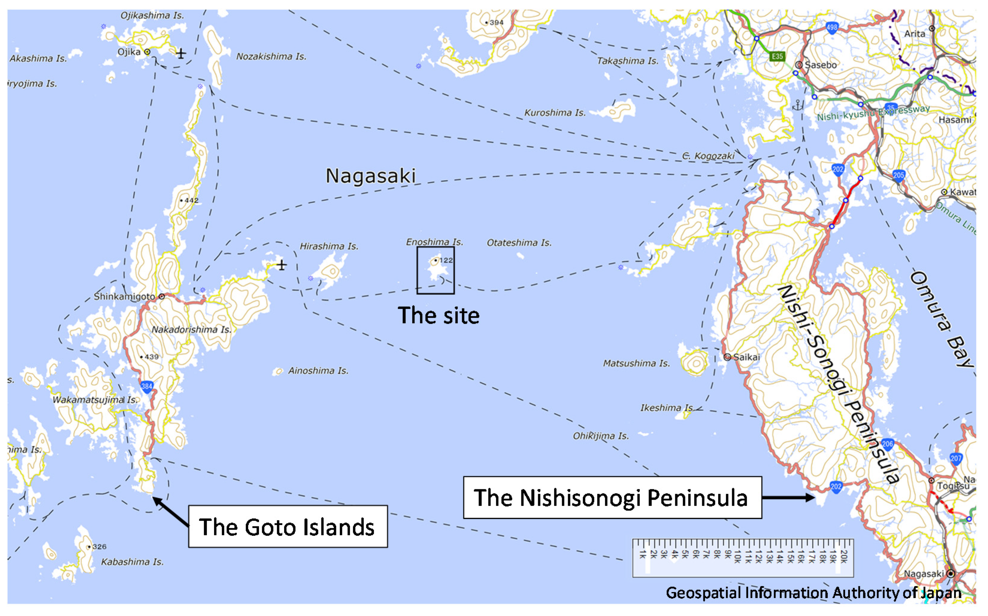
2. Overview of the Investigated Site
3. Analysis of the Measurement Data
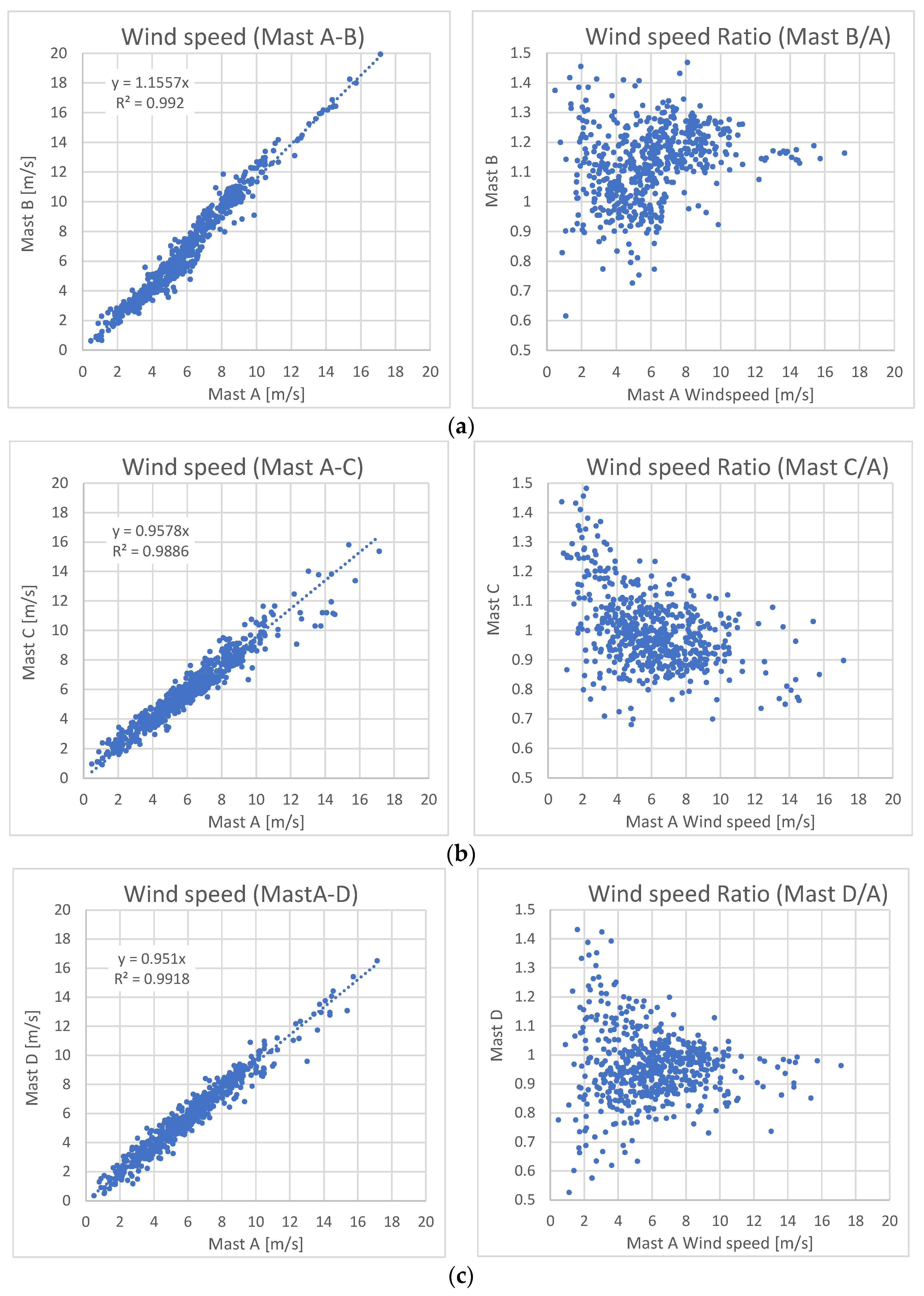
3.1. Correlation and Wind Speed Ratio for Each Mast
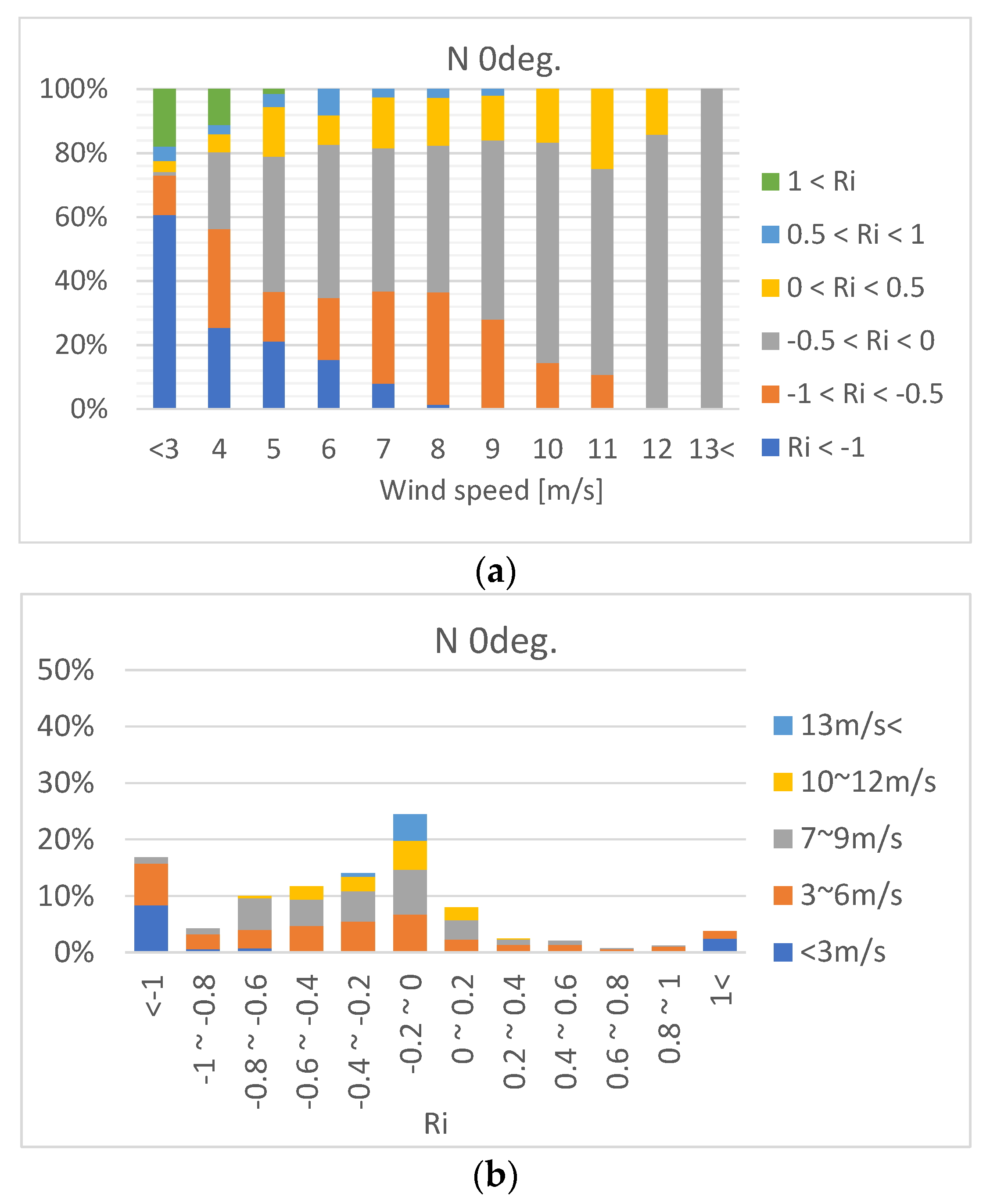
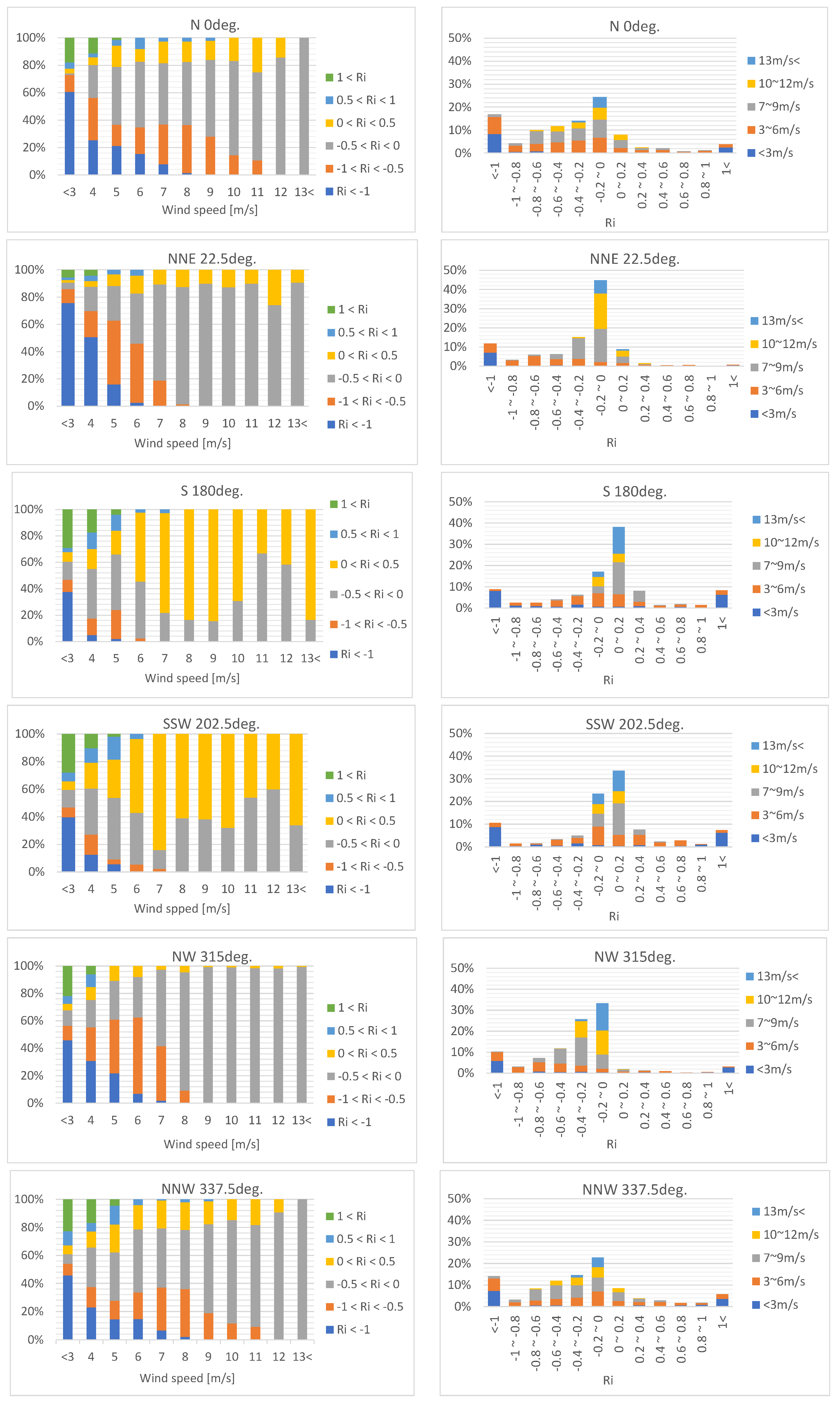
3.2. Distribution of Annual Atmospheric Stability
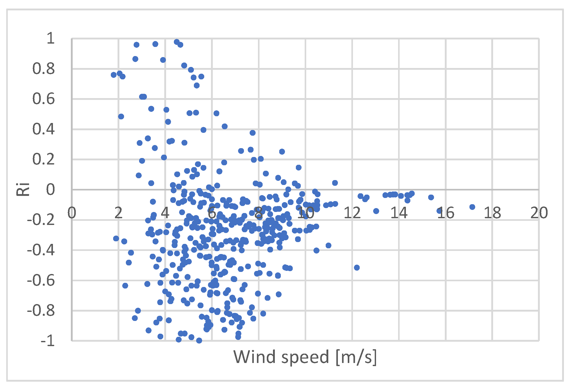
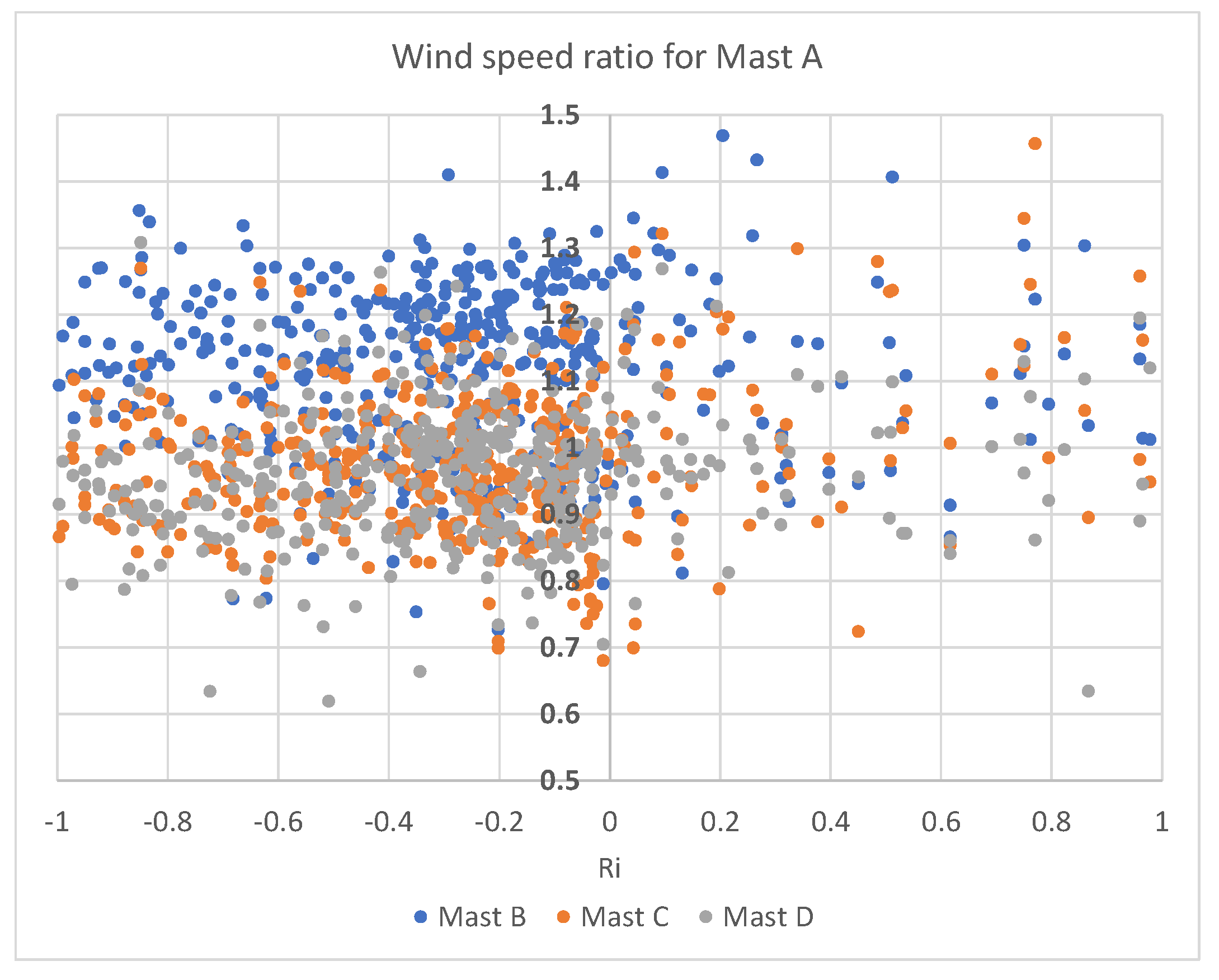
3.3. Investigation in Relation to the Variation of Atmospheric Stability
3.4. Decision of Atmospheric Stability for Numerical Simulation
4. Numerical Simulation
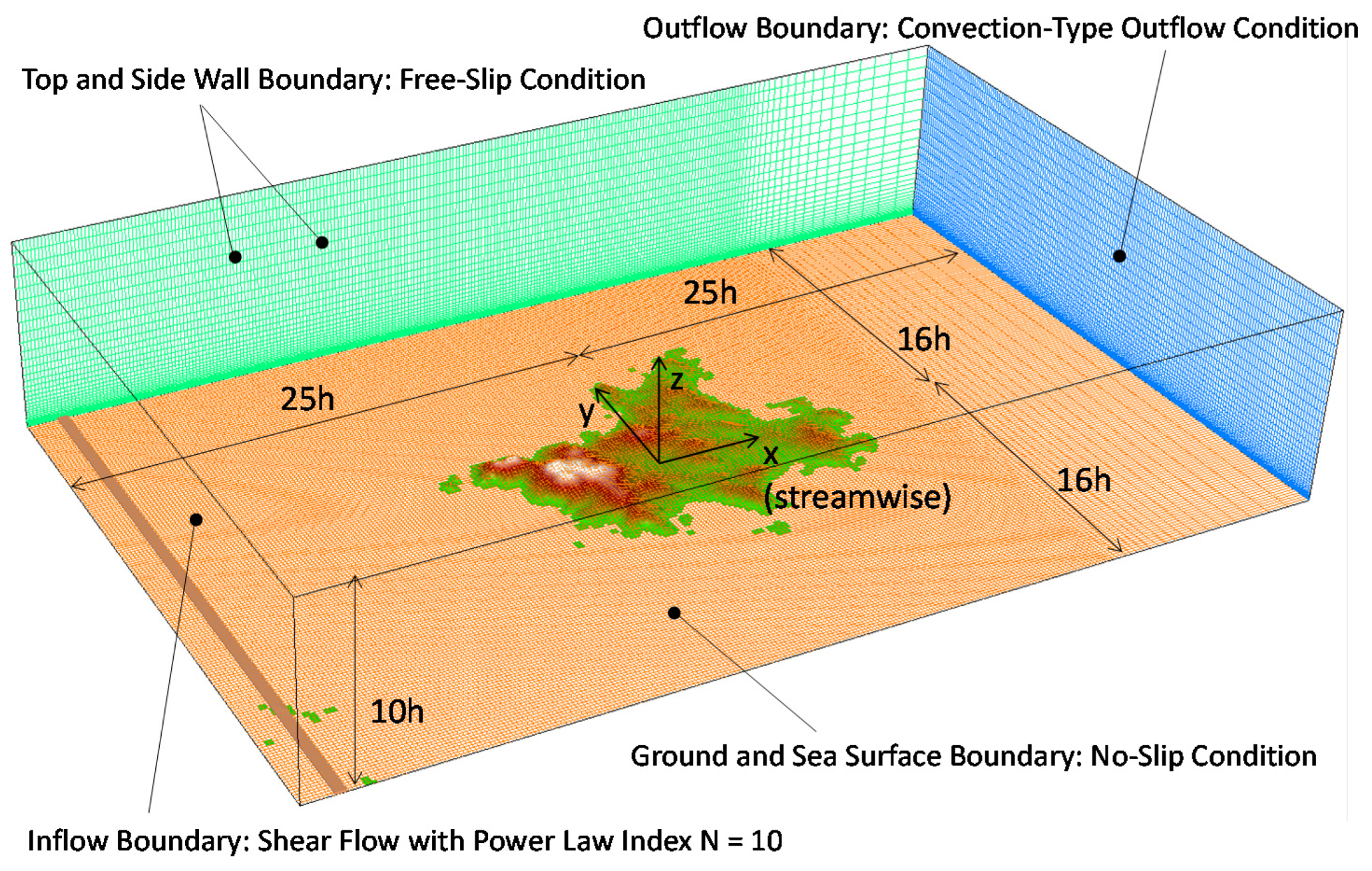
4.1. Summary of the Numerical Simulation Methods
4.2. Results and Discussions
4.2.1. Validation of Vertical Profile
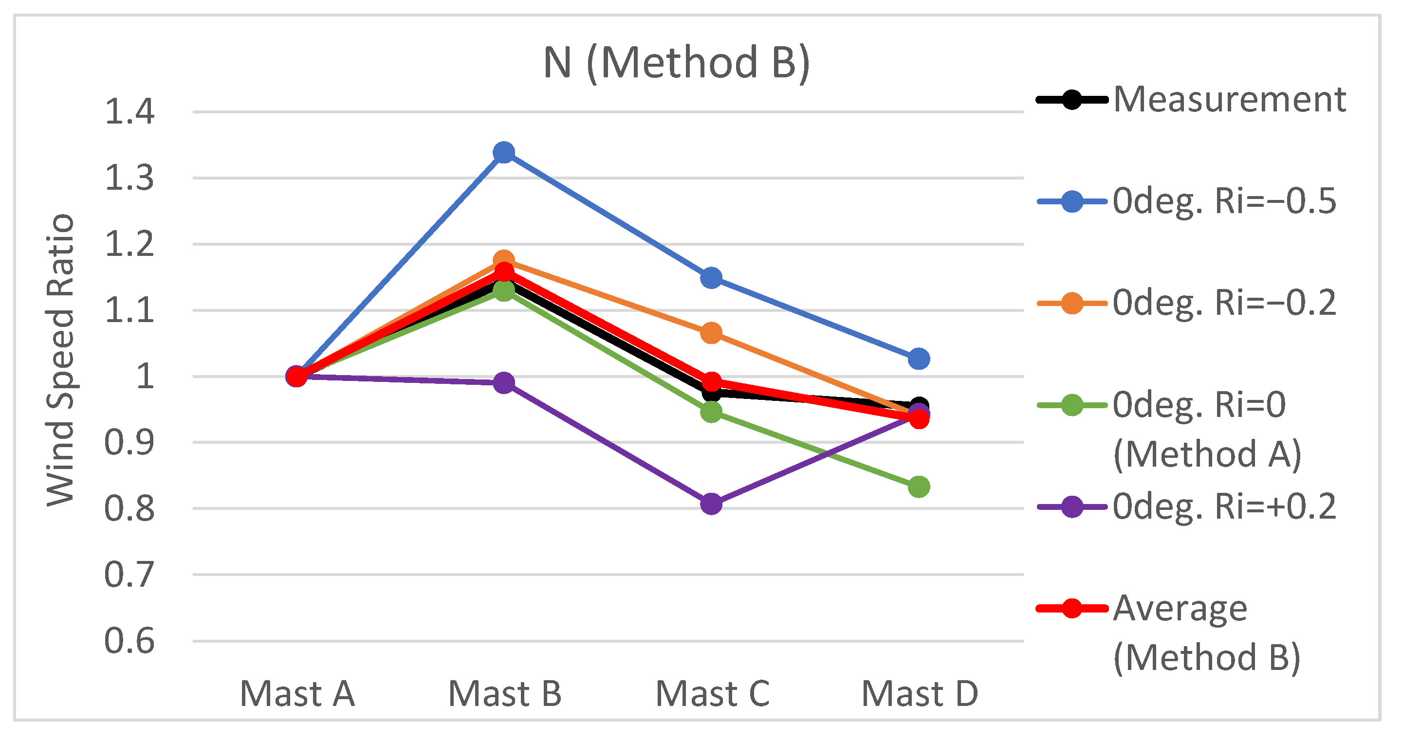
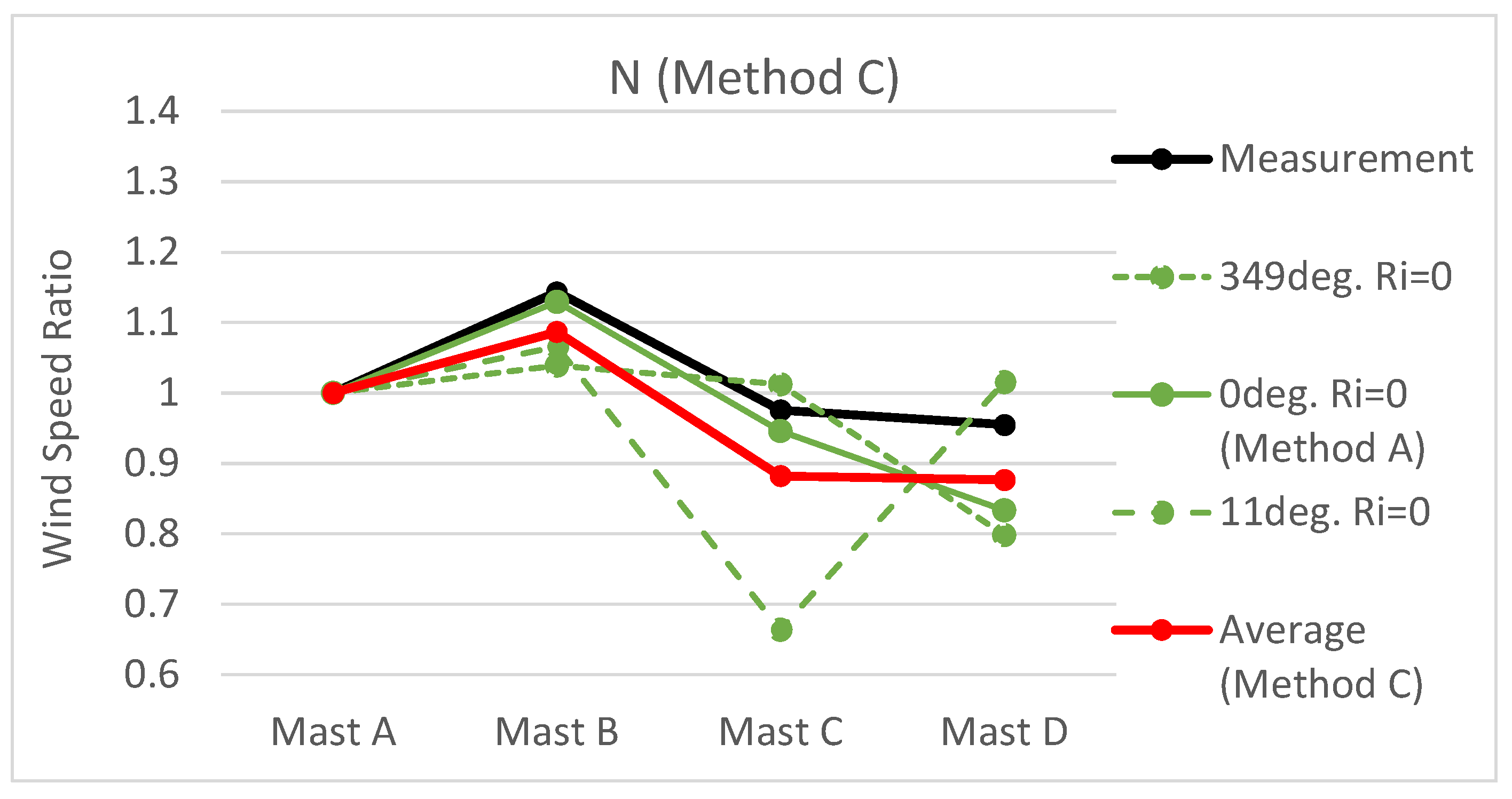
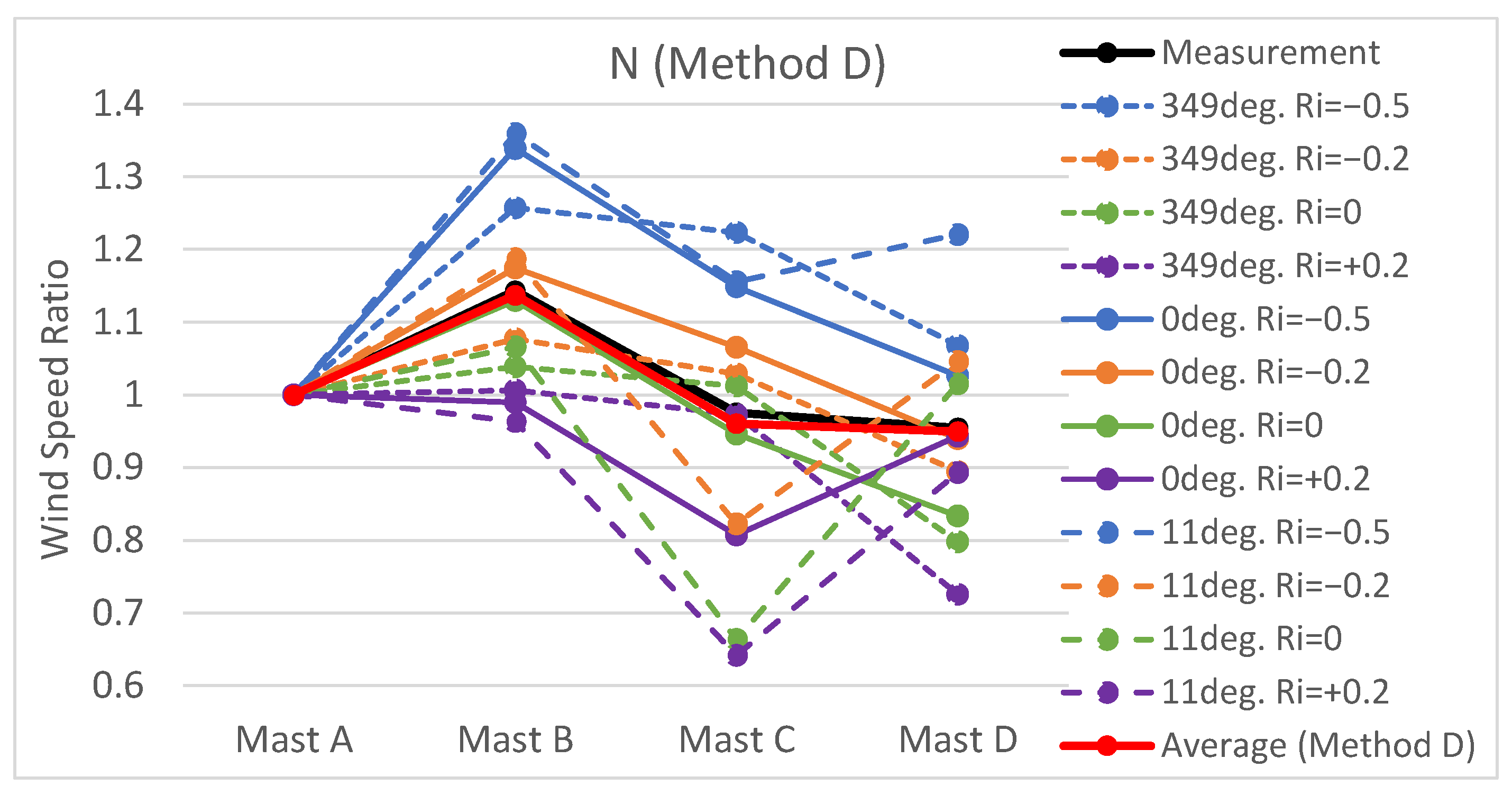
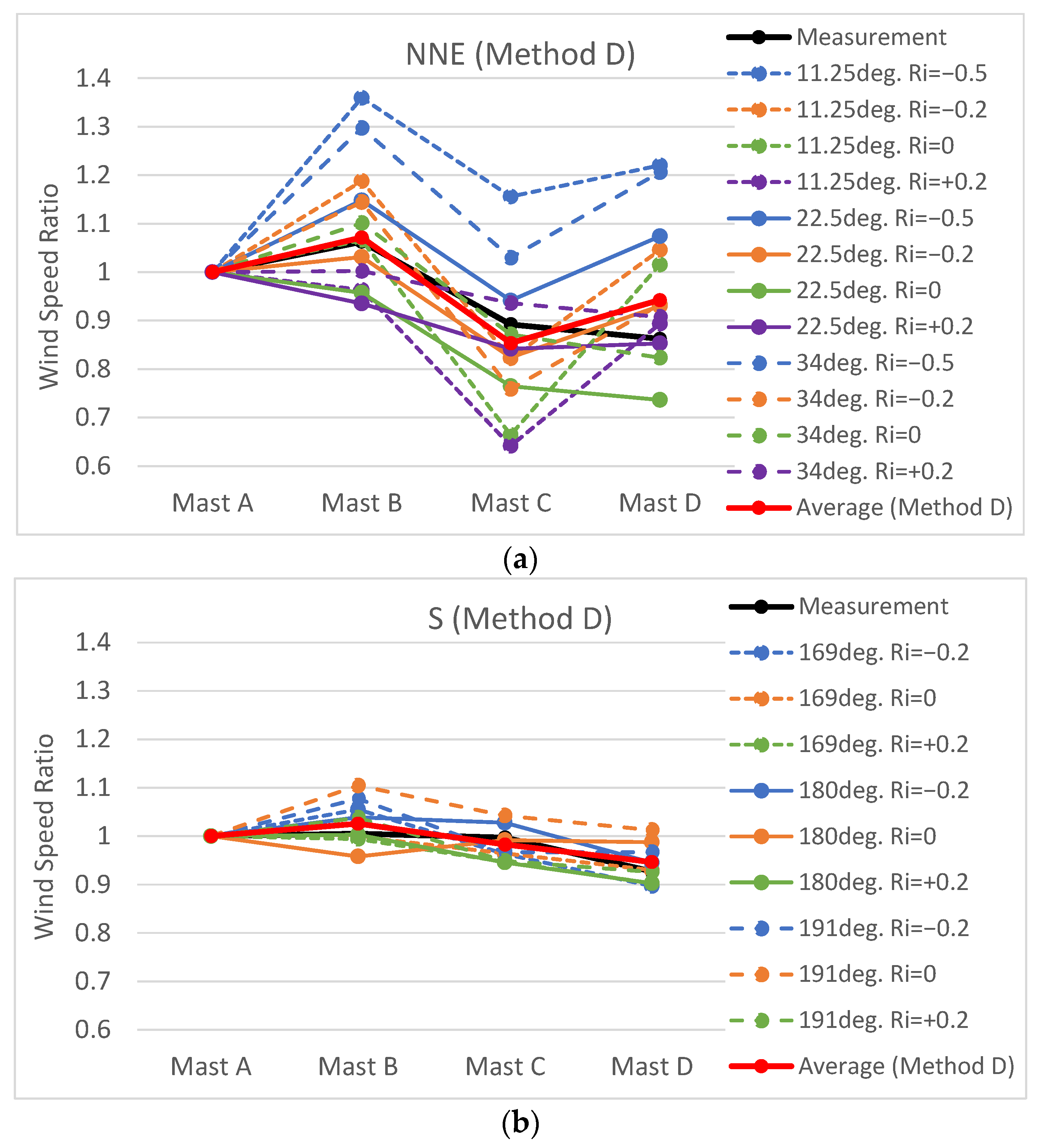
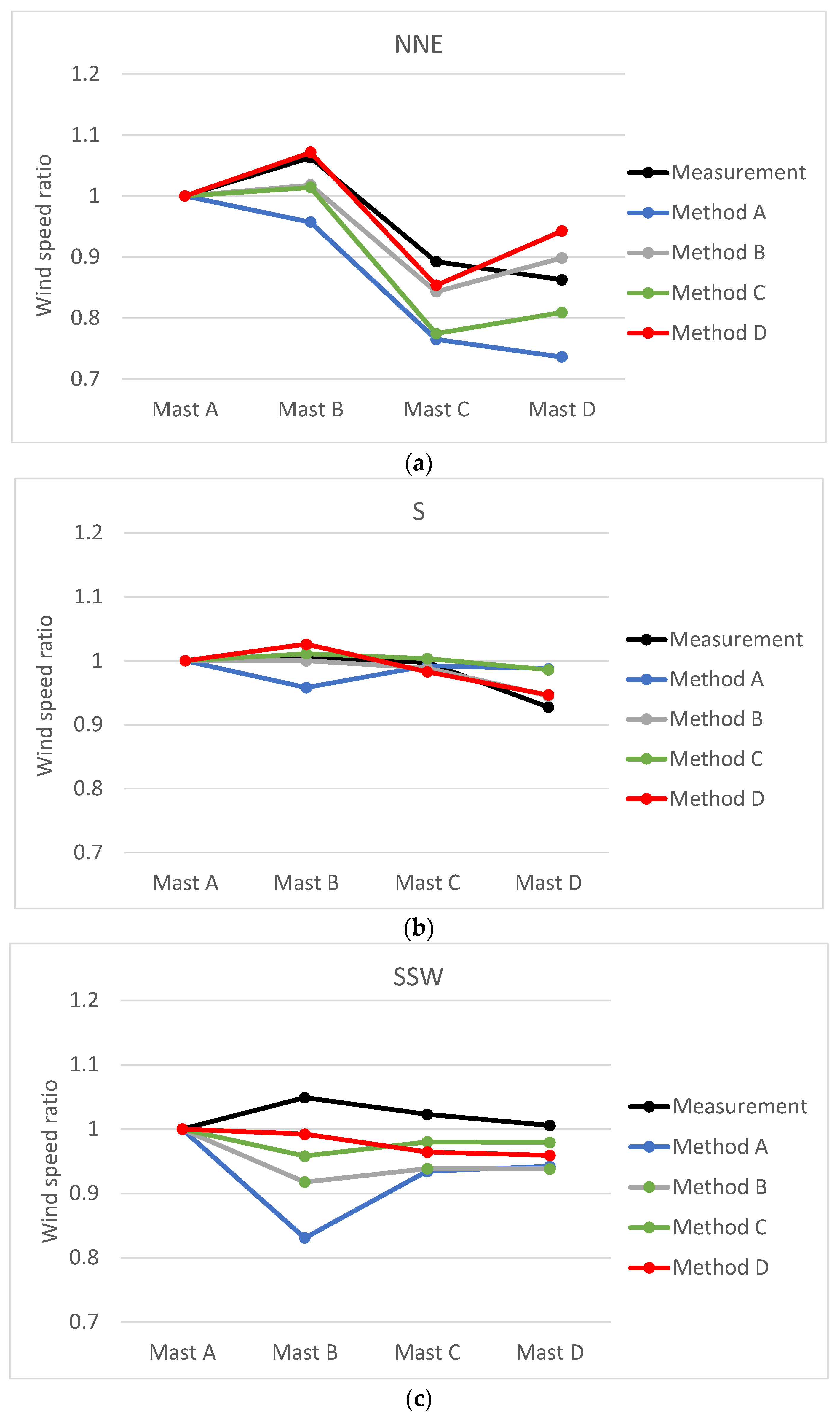
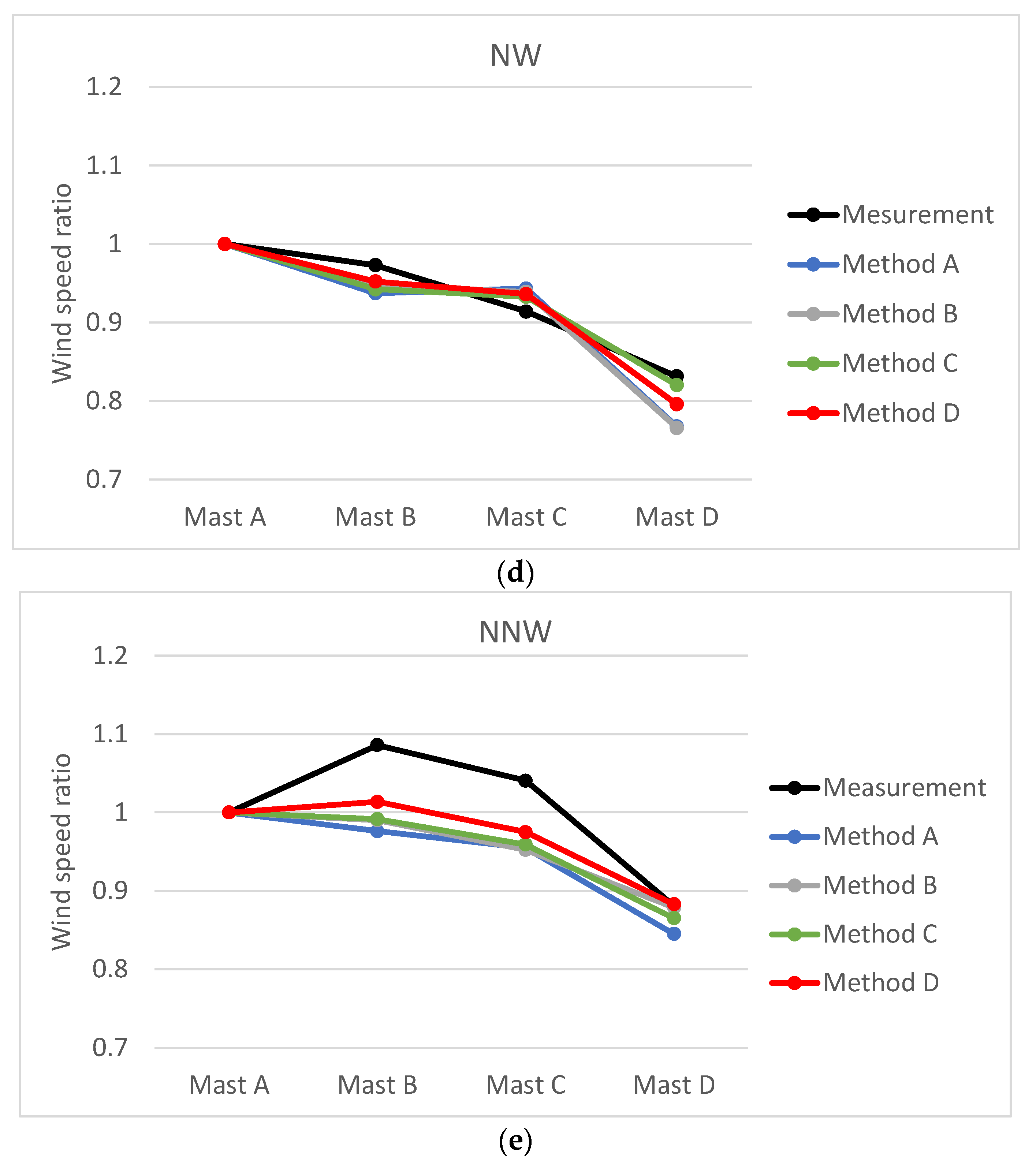
4.2.2. Validation of Wind Speed Ratio
4.2.3. Wind Speed Distribution in a Numerical Simulation
5. Conclusions
Author Contributions
Funding
Institutional Review Board Statement
Informed Consent Statement
Data Availability Statement
Acknowledgments
Conflicts of Interest
Nomenclature
| Ri | Richardson number |
| U | streamwise wind speed [m/s] |
| x | streamwise coordinate [m] |
| y | streamwise perpendicular coordinate [m] |
| z | vertical coordinate [m] |
| θbottom | sea surface temperature [K] |
| θin | in flow temperature [K] |
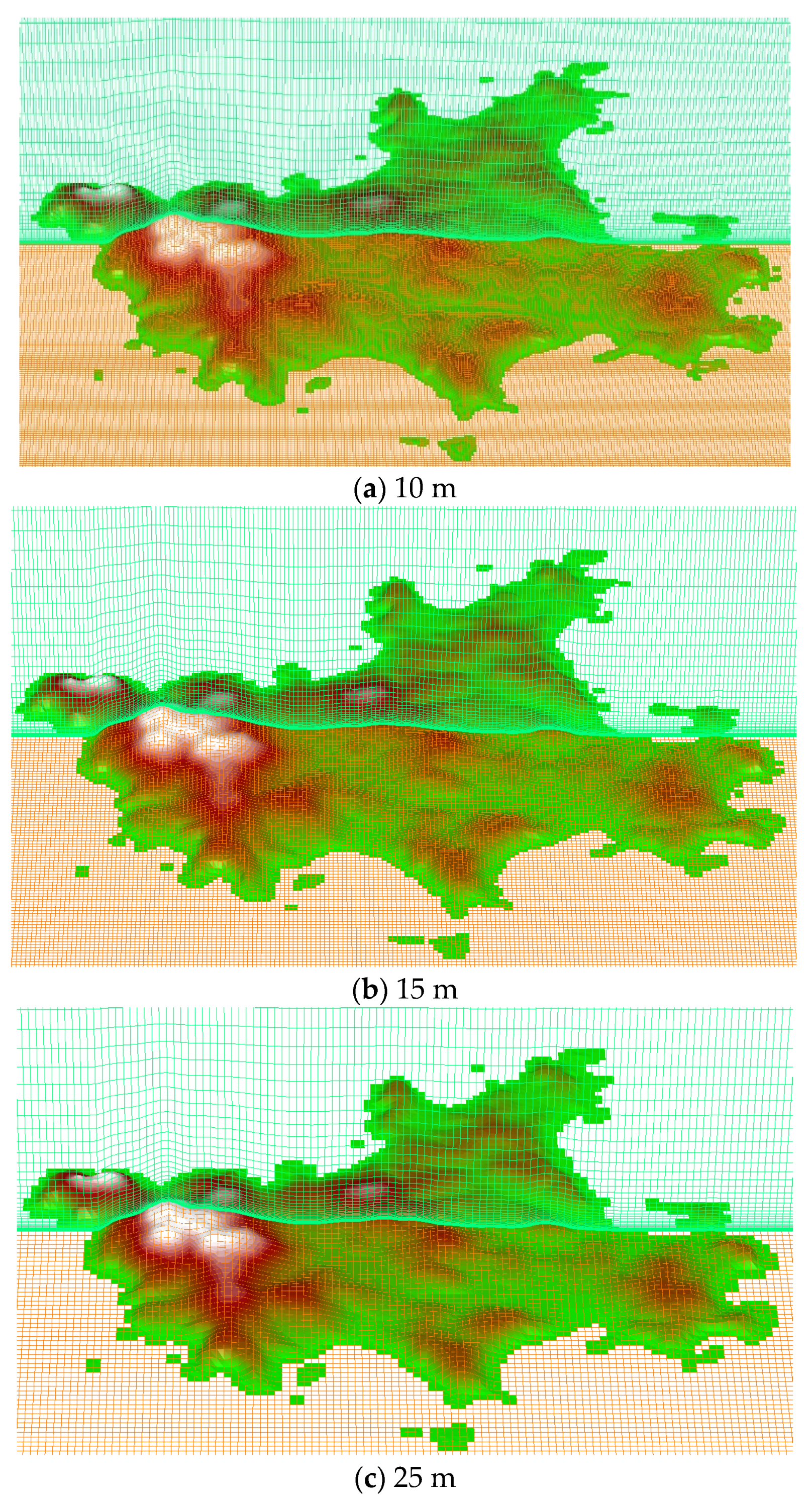
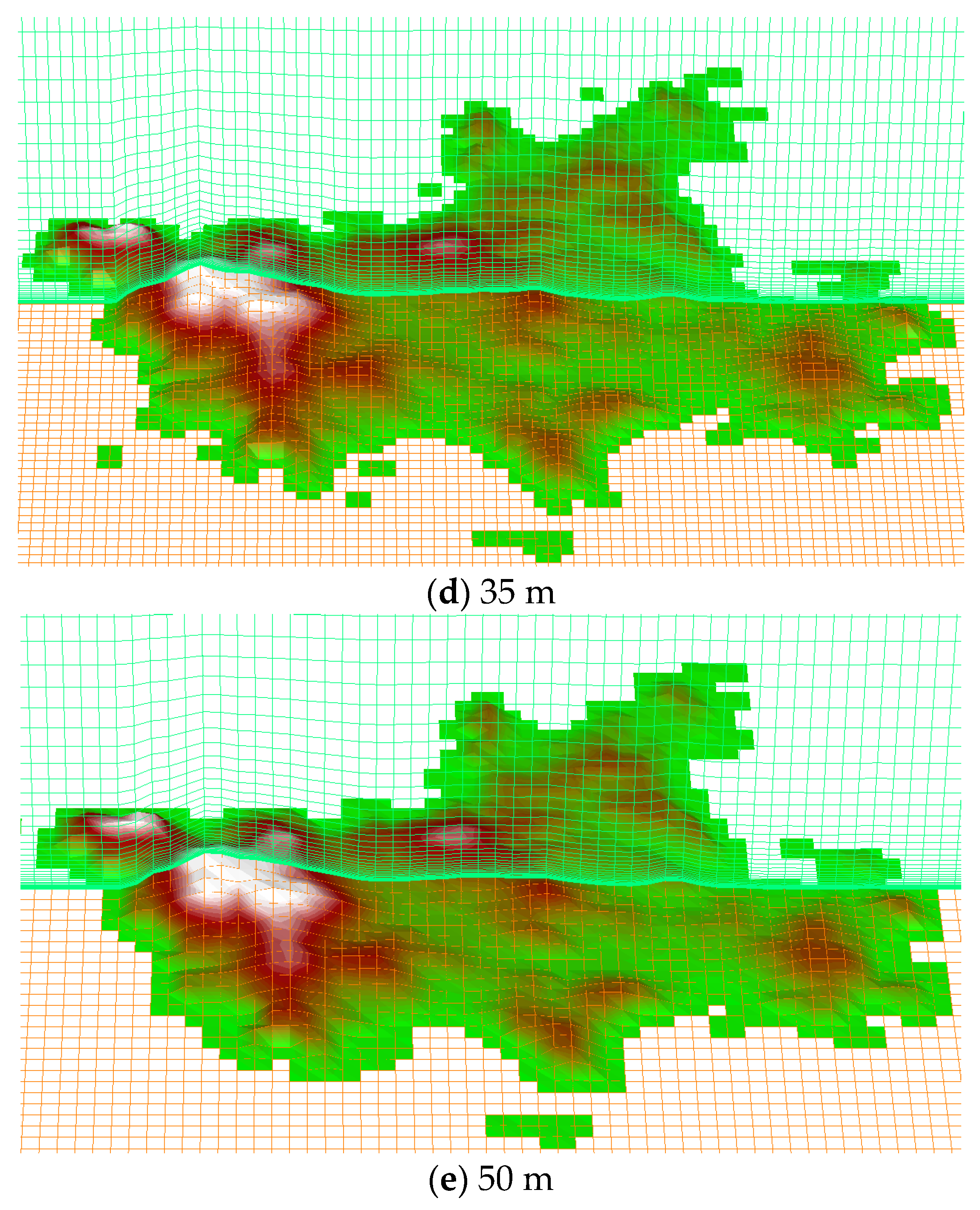
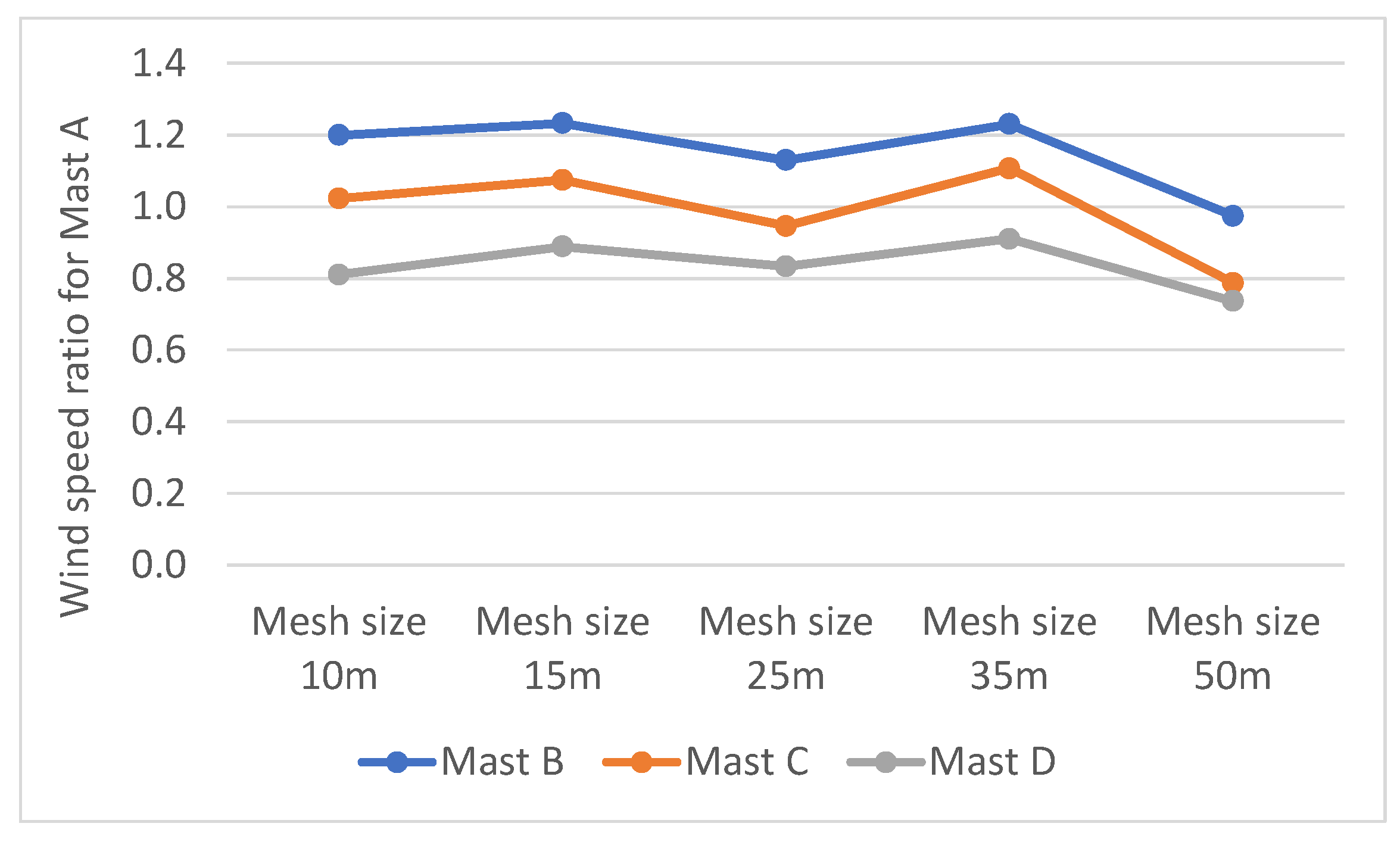
Appendix A. Effect of Grid Resolution on Wind Speed Ratio
References
- Japan Wind Power Association Report. Available online: https://jwpa.jp/en/information/6105/ (accessed on 30 November 2018).
- Stull, R.B. An Introduction to Boundary Layer Meteorology; Kluwer Academic Publishers: Dordrecht, The Netherlands, 1998. [Google Scholar]
- Uchida, T.; Takakuwa, S. Numerical Investigation of Stable Stratification Effects on Wind Resource Assessment in Complex Terrain. Energies 2020, 13, 6638. [Google Scholar] [CrossRef]
- Porté-Agel, F.; Bastankhah, M.; Shamsoddin, S. Wind-Turbine and Wind-Farm Flows: A Review. Bound. Layer Meteorol. 2020, 174, 1–59. [Google Scholar] [CrossRef] [PubMed] [Green Version]
- Dörenkämper, M.; Witha, B.; Steinfeld, G.; Heinemann, D.; Kühn, M. The impact of stable atmospheric boundary layers on wind-turbine wakes within offshore wind farms. J. Wind. Eng. Ind. Aerodyn. 2015, 144, 146–153. [Google Scholar] [CrossRef] [Green Version]
- Abkar, M.; Porté-Agel, F. The Effect of Free-Atmosphere Stratification on Boundary-Layer Flow and Power Output from Very Large Wind Farms. Energies 2013, 6, 2338–2361. [Google Scholar] [CrossRef] [Green Version]
- Lu, H.; Porté-Agel, F. Large-eddy simulation of a very large wind farm in a stable atmospheric boundary layer. Phys. Fluids 2011, 23, 065101. [Google Scholar] [CrossRef]
- Weather Research and Forecasting Model. Available online: https://www.mmm.ucar.edu/weather-research-and-forecasting-model (accessed on 2 December 2021).
- Uchida, T.; Li, G. Comparison of RANS and LES in the Prediction of Airflow Field over Steep Complex Terrain. Open J. Fluid Dyn. 2018, 8, 286–307. [Google Scholar] [CrossRef] [Green Version]
- FY2020 Promising Sea Areas and Sites Selected for Future Designation of Project Target Areas. Available online: https://www.meti.go.jp/english/press/2020/0703_003.html (accessed on 1 April 2021).
- JRE and wpd to Conduct Joint Enterprise in Saikai Enoshima Offshore Wind Power Project. Available online: https://www.jre.co.jp/news/pdf/news_20210907_E.pdf (accessed on 7 September 2021).
- ERA5. Available online: https://www.ecmwf.int/en/forecasts/datasets/reanalysis-datasets/era5 (accessed on 1 September 2020).
- Uchida, T.; Ohya, Y. Micro-siting technique for wind turbine generators by using large-eddy simulation. J. Wind. Eng. Ind. Aerodyn. 2008, 96, 2121–2138. [Google Scholar] [CrossRef]
- Uchida, T. Computational Fluid Dynamics Approach to Predict the Actual Wind Speed over Complex Terrain. Energies 2018, 11, 1694. [Google Scholar] [CrossRef] [Green Version]
- Uchida, T.; Sugitani, K. Numerical and Experimental Study of Topographic Speed-Up Effects in Complex Terrain. Energies 2020, 13, 3896. [Google Scholar] [CrossRef]
- Uchida, T.; Takakuwa, S. A Large-Eddy Simulation-Based Assessment of the Risk of Wind Turbine Failures Due to Terrain-Induced Turbulence over a Wind Farm in Complex Terrain. Energies 2019, 12, 1925. [Google Scholar] [CrossRef] [Green Version]
- Rodrigo, J.S.; Gancarski, P.; Arroyo, R.B.; Moriarty, P.; Chuchfield, M.; Naughton, J.W.; Hansen, K.S.; Machefaux, E.; Koblitz, T.; Maguire, E.; et al. IEA-Task 31 WAKEBENCH: Towards a protocol for wind farm flow model evaluation. Part 1: Flow over-terrain models. J. Phys. Conf. Ser. 2014, 524, 012105. [Google Scholar] [CrossRef] [Green Version]
- Moriarty, P.; Rodrigo, J.S.; Gancarski, P.; Chuchfield, M.; Naughton, J.W.; Hansen, K.S.; Machefaux, E.; Maguire, E.; Castellani, F.; Terzi, L.; et al. IEA-Task 31 WAKEBENCH: Towards a protocol for wind farm flow model evaluation. Part 2: Wind farm wake models. J. Phys. Conf. Ser. 2014, 524, 012185. [Google Scholar] [CrossRef] [Green Version]
- MEASNET. Evaluation of Site-Specific Wind Conditions, Version 2. April 2016. Available online: https://www.measnet.com/wp-content/uploads/2016/05/Measnet_SiteAssessment_V2.0.pdf (accessed on 1 April 2021).
- International Electrotechnical Commission. IEC 61400-12-1:2017 ed2. Wind Energy Generation Systems—Part 12-1: Power Performance Measurements of Electricity Producing Wind Turbines. Available online: https://webstore.iec.ch/publication/26603 (accessed on 1 April 2021).
- Uchida, T. Numerical Investigation of Terrain-Induced Turbulence in Complex Terrain by Large-Eddy Simulation (LES) Technique. Energies 2018, 11, 2638. [Google Scholar] [CrossRef] [Green Version]


| N | NNE | S | SSW | NW | NNW | |
|---|---|---|---|---|---|---|
| Ri = −0.5 | √ | √ | - | - | √ | √ |
| Ri = −0.2 | √ | √ | √ | √ | √ | √ |
| Ri = 0 | √ | √ | √ | √ | √ | √ |
| Ri = +0.2 | √ | √ | √ | √ | - | √ |
| Atmospheric Stability | Inflow Wind Direction | |
|---|---|---|
| Method A | Neutral | Center (0 deg.) |
| Method B | Simple average (Ri = −0.5, −0.2, 0, +0.2) | Center (0 deg.) |
| Method C | Neutral | Weighted average (0 deg., 11 deg., 349 deg.) |
| Method D | Simple average (Ri = −0.5, −0.2, 0, +0.2) | Weighted average (0 deg., 11 deg., 349 deg.) |
| Method A | Method B | Method C | Method D | |
|---|---|---|---|---|
| Error of Mast B | −1.2% | 1.3% | −4.9% | −0.5% |
| Error of Mast C | −3.0% | 1.7% | −9.6% | −1.5% |
| Error of Mast D | −12.7% | −2.0% | −8.2% | −0.5% |
| Averaged absolute error | 5.6% | 1.7% | 7.6% | 0.9% |
| Max of absolute error | 12.7% | 2.0% | 9.6% | 1.5% |
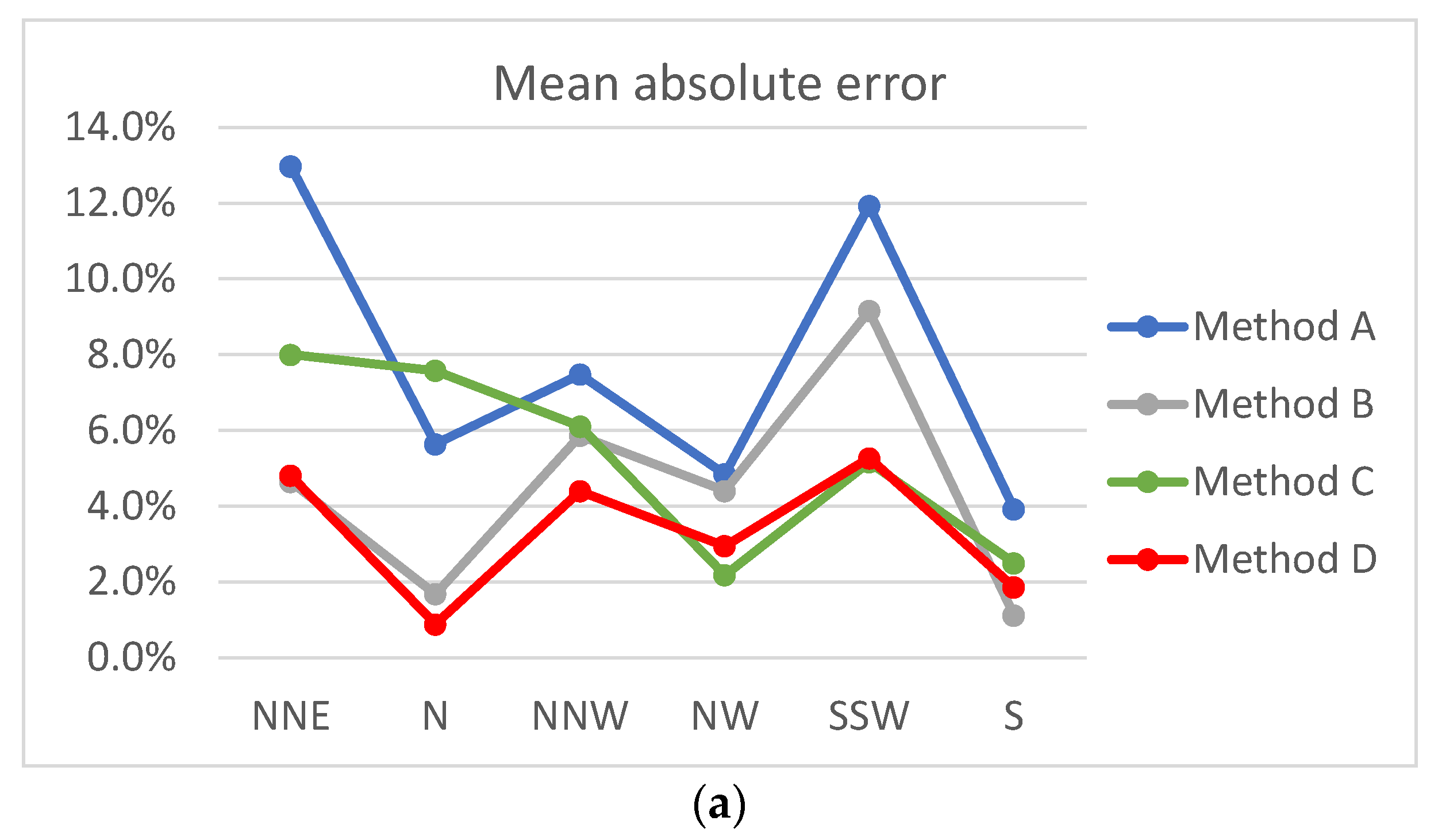
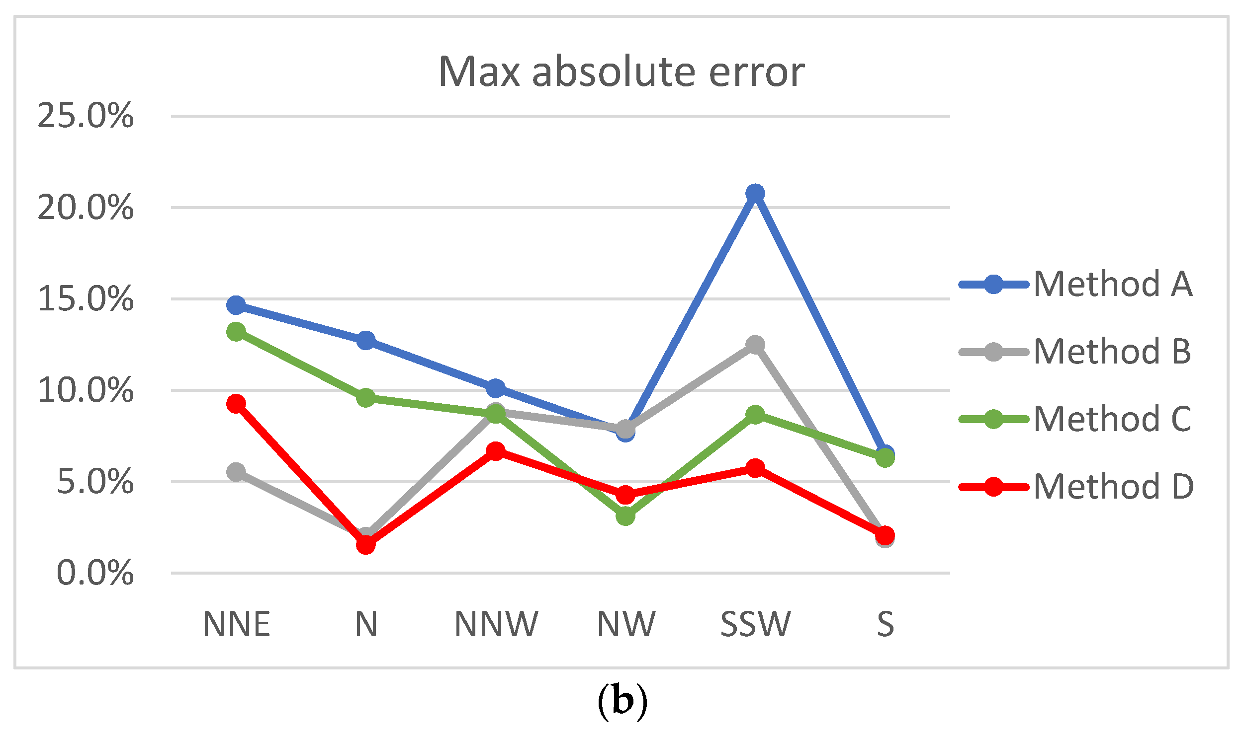
| Method | A | B | C | D |
|---|---|---|---|---|
| Mean absolute error | 7.8% | 4.5% | 5.3% | 3.4% |
| Mean of the maximum absolute error for each wind direction sector | 12.1% | 6.4% | 8.3% | 4.9% |
| Maximum absolute error | 20.8% | 12.5% | 13.2% | 9.3% |
Publisher’s Note: MDPI stays neutral with regard to jurisdictional claims in published maps and institutional affiliations. |
© 2022 by the authors. Licensee MDPI, Basel, Switzerland. This article is an open access article distributed under the terms and conditions of the Creative Commons Attribution (CC BY) license (https://creativecommons.org/licenses/by/4.0/).
Share and Cite
Takakuwa, S.; Uchida, T. Improvement of Airflow Simulation by Refining the Inflow Wind Direction and Applying Atmospheric Stability for Onshore and Offshore Wind Farms Affected by Topography. Energies 2022, 15, 5050. https://doi.org/10.3390/en15145050
Takakuwa S, Uchida T. Improvement of Airflow Simulation by Refining the Inflow Wind Direction and Applying Atmospheric Stability for Onshore and Offshore Wind Farms Affected by Topography. Energies. 2022; 15(14):5050. https://doi.org/10.3390/en15145050
Chicago/Turabian StyleTakakuwa, Susumu, and Takanori Uchida. 2022. "Improvement of Airflow Simulation by Refining the Inflow Wind Direction and Applying Atmospheric Stability for Onshore and Offshore Wind Farms Affected by Topography" Energies 15, no. 14: 5050. https://doi.org/10.3390/en15145050
APA StyleTakakuwa, S., & Uchida, T. (2022). Improvement of Airflow Simulation by Refining the Inflow Wind Direction and Applying Atmospheric Stability for Onshore and Offshore Wind Farms Affected by Topography. Energies, 15(14), 5050. https://doi.org/10.3390/en15145050