Adaptive Second-Order Sliding Mode Control of Buck Converters with Multi-Disturbances

Abstract

In this paper, a novel adaptive second-order sliding mode (2-SM) control approach, based on online zero-crossing detection, was proposed to solve the problems of the chattering and fixed control gain for buck converters with multi-disturbances. In modeling, the possible parameter perturbations and external disturbances of the converter system were contained. Instead of the traditional first-order sliding mode (1-SM), the twisting algorithm with 2-SM was adopted for the controller design, which could overcome the chattering problem and realize control continuity. Meanwhile, a novel adaptive mechanism was introduced to replace the conventional fixed control gain by time-varying control gain, the idea of which is to calculate the number of the zero-crossing points of the sliding surface online. As a result, the control magnitude of the improved controller could be reduced to a minimal admissible level, and the steady error of the output voltage could converge to the expected value. Furthermore, the robust stability of the converter system with multi-disturbances wads investigated. Comparative simulations and experiments validated the advantages of this paper as offering better robustness and control performance.

1. Introduction

As a kind of DC-DC power converter, the buck type has been widely used in various fields, due to its simple circuit topology, high efficiency and reliability [1,2]. Since buck converters generally consist of such components as the inductor, capacitor, diode and power switches (e.g., IGBT, MOSFET), they are characterized by time-varying nonlinearity. In practical applications, the traditional control approaches are mainly focused on PID [3] and state feedback control [4], and their control laws are generally constructed as the linear combination of the measured voltages and currents. Although these approaches are simple and easy to implement, they are sensitive to parameter perturbations and external disturbances, leading to poor robustness, and poor dynamic and static performances. For example, in [5], the magnetic characteristics of inductors were proved to vary greatly in the presence of large magnetic flux density. In [6], the variations of load resistor and input voltage were proved not to be neglected, especially in the case of large signal operation. Therefore, the control of buck converters with satisfactory performance is still a challenging issue to be addressed, especially in the case of parameter perturbations and external disturbances [7,8].

As an effective nonlinear and robust control approach, a large amount of literature has proved that sliding mode (SM) control is more suitable for the switching control of buck converters. On the one side, the SM controller can replace the traditional pulse width modulation (PWM) and realize direct ON/OFF switching control of the converters by triggering the gate of the controllable power switches. As a result, it is simple and no extra modulation circuits are needed [9,10]. On the other side, SM is inherently nonlinear, which differs from the approximate nonlinearity of the substitutes, like the fuzzy control [11,12], neural network [13,14] and other intelligent control approaches [15,16,17]. As a result, the control performances under SM control are better; besides, the amount and time involved in the calculation can also be saved. A review of recent SM applications in power converters can be referred to [18]. For example, in [19], a linear sliding mode (LSM) controller was proposed to guarantee the asymptotic convergence of the output voltage; in [20], a terminal sliding mode (TSM) control approach was proposed to improve steady accuracy and response speed by introducing finite-time convergence; in [21], a non-singular terminal sliding mode (NTSMC) control approach was proposed to realize wide-range voltage regulation of the buck converters, due to its global finite-time convergence. Although the above SM approaches are the three commonly used types in practice, they belong to the traditional first-order SM (1-SM) [22,23,24]. Attention should be paid to the chattering problem [25], which is harmful to the stability and control performances of the system. It is closely related to switching nonlinearity, denoted as the signum function, i.e., sgn(·). In other words, when the system slides along the predesigned surface, its trajectory switches back and forth under the function of the discontinuous control law, leading to the undesired chattering phenomenon [26,27].

In order to solve the chattering problem, two approaches can generally be used: continuous approximation and high-order sliding mode (HOSM). For the former, a saturation function [28] or a sigmoid-like function [29] or the combination of SM with intelligent control [30] can be generally introduced into a boundary layer around the sliding surface to smoothen the discontinuity of SM control law. However, this approach suffers from poor accuracy and the loss of robustness inside of the predesigned sliding surface. Meanwhile, despite the time-varying control magnitude, such intelligent control technology as the fuzzy logic [31] and neural network [32] depend on the experience of engineers, and the system stability cannot be guaranteed. For the latter, HOSM can be regarded as the extension of the traditional 1-SM in the sense of relative degree [33,34]. Its idea is to impose the switching control on the first-order derivative of the sliding variable. As a result, the chattering elimination and the expected control continuity can be achieved by the integral operation or the low-pass filtering of the switching control. At present, second-order SM (2-SM) is the most popular HOSM applied in practice. More specifically, the twisting algorithm [35], sub-optimal algorithm [36], and super-twisting algorithm [37] are the often-used 2-SM. However, when facing unknown and complex disturbances, these algorithms suffer from overestimation and unnecessary control magnitudes, leading to the degradation of performances and efficiency.

In order to solve the problem of the unnecessary and fixed control gain of 2-SM, the adaptive mechanism was introduced as an effective solution to achieve time-varying control gains [38]. At present, the often-used adaptive mechanisms can be classified into three kinds, based on the Lyapunov stability theory, intelligent control technology and the switching trajectory, respectively. For the first type, its idea is to achieve a time-varying control gain on the premise of system stability. For example, in [39], an observer-based 2-SM approach was proposed, following the guaranteed robust stability of the observer and the controller based on the Lyapunov stability theory; in [40,41,42], several adaptive 2-SM approaches were applied into uncertain or disturbing systems in practice, respectively. Compared with nominal systems, application of the adaptive mechanism is more significant. However, despite the fact that the control gain can dynamically decrease as the system converges to the equilibrium point, its relationship with the control performance is difficult to obtain. For the second type, its idea is to integrate such intelligent control technology as fuzzy logic and neural network with the 2-SM controller to achieve adaptive control magnitude, which changes as the states change [43,44]. However, it is heavily reliant on the prior evaluation of experts. The third type takes advantage of the inherent “switching” nature of real (non-ideal) sliding modes and its adaptive mechanism depends on counting the zero-crossing points of the sliding variable in a certain time interval [45]. Therefore, its merits lie in the capability of online calculation, instead of traditional offline settings. Since it can adjust and maintain the control magnitude at the minimum admissible level, it is significant for engineering practice. However, some issues concerning the online zero-crossing mechanism still need to be investigated, especially for robust stability when facing the complex disturbances of buck converters.

In this paper, a novel adaptive 2-SM control approach was proposed on the basis of online zero-crossing detection to improve the control performances of buck converters with disturbances. The problems of the chattering and the fixed control gain were two key issues addressed. To be specific, the main contributions of this paper can be concluded as follows:

• Without loss of generality, the possible parameter perturbations and external disturbances of the buck converters are all considered in modeling;
• The robust stability of the converter system is investigated;
• The adaptive mechanism of online zero-crossing detection is investigated;
• The control magnitude of the controller can vary to a minimal admissible level, and the steady error of the output voltage can converge to the expected value.

This paper is organized as follows. In Section 2, the possible parameter perturbations and external disturbances of buck converters are considered in modeling. In Section 3, the twisting algorithm [35] is chosen as an example of the traditional 2-SM to design a controller for the buck converter. In Section 4, an improved twisting algorithm is proposed by combining with the adaptive mechanism of online zero-crossing detection, following its robust stability analysis. Finally, the comparative simulations, experiments and concluding remarks are given in Section 5 and Section 6, respectively.

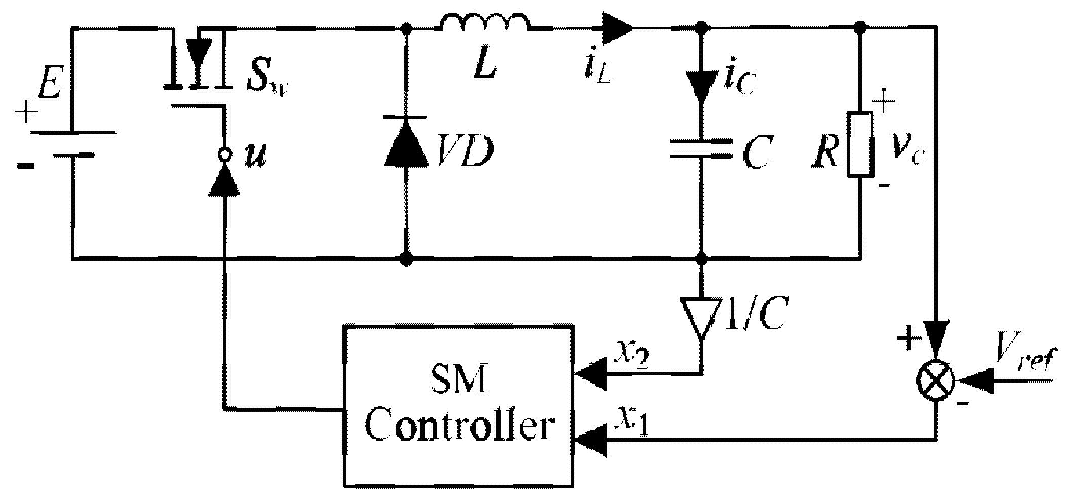
2. Model of Buck Converters with Multi-Disturbances

Figure 1 gives the structure diagram of SM controlled converters. The converter circuit consists of a DC input voltage source E, a diode VD, a filter inductor L and capacitor C, a load resistor R and a controlled power switch S_w; i_L and i_C are the currents flowing through the inductor and the capacitor, respectively; v_c is the transient value of the output voltage.

2.1. Modeling of Buck Converters with Multi-Disturbances

In practical applications, buck converters generally work in the following conditions:

• Continuous conduction mode (CCM), i.e., the inductor current i_L ≠ 0;
• DC input voltage 0 < E < E_max, where E_max is its maximum;
• MOSFET or IGBT act as the power switch S_w, the ON/OFF switching control of which is implemented by triggering its gate pole.

Here we define u = 1 and u = 0 as the ON and OFF statuses of the power switch S_w, respectively. Based on Kirchhoff’s circuit law, the dynamic equation of the converter system can be given as

$$\{\begin{array}{l}\frac{d{i}_L}{dt}=\frac{1}{L}\left(uE-v_c\right)\\ \frac{d{v}_c}{dt}=\frac{1}{C}\left(i_L-\frac{v_c}{R}\right)\end{array}$$

(1)

Furthermore, we define V_ref as the DC reference value of the output voltage v_c, x₁ and x₂ are the output voltage error and its derivative, i.e.,

$$\{\begin{array}{l}{x}_1=v_c-V_{ref}\\ x_2={\dot{x}}_1={\dot{v}}_c\end{array}$$

(2)

In this paper, the possible parameter perturbations and external disturbances of buck converters were considered, including the variations of input and reference output voltage (i.e., ∆E and ∆V_ref), parameter uncertainties of load resistor, inductor, and capacitor (i.e., ∆R, ∆L and ∆C), and time-varying external disturbances d₁(t) and d₂(t). Therefore, (1) and (2) could be changed to

$$\{\begin{array}{l}\frac{d{i}_L}{dt}=\frac{1}{L+\Delta L}\left[u(\Delta E+E)-v_c\right]+d_1(t)\\ \frac{d{v}_c}{dt}=\frac{1}{C+\Delta C}\left(i_L-\frac{v_c}{R+\Delta R}\right)+d_2(t)\end{array}$$

(3)

Or the alternative form

$$\{\begin{array}{l}{\dot{x}}_1=x_2\\ {\dot{x}}_2={\beta }_1{x}_1+{\beta }_2{x}_2+{\beta }_{3}u+{\beta }_4\left(t\right)\end{array}$$

(4)

where the lumped disturbing matrices β₁, β₂, β₃ and β₄ were denoted as

$$\begin{array}{l}{\beta }_1=\frac{-1}{\left(C+\Delta C\right)\left(L+\Delta L\right)},\begin{array}{cc}& \end{array}{\beta }_2=\frac{-1}{\left(C+\Delta C\right)\left(R+\Delta R\right)}\\ {\beta }_3=\frac{E+\Delta E}{\left(C+\Delta C\right)\left(L+\Delta L\right)},\begin{array}{cc}& \end{array}{\beta }_4\left(t\right)=\frac{d_1\left(t\right)}{C+\Delta C}+{\dot{d}}_2\left(t\right)-\frac{V_{ref}+\Delta V_{ref}}{\left(C+\Delta C\right)\left(L+\Delta L\right)}\end{array}$$

(5)

The mathematical expression of the buck converter in (5) covered all the model uncertainties and external disturbances. However, attention should be paid to the fact that there might be individual, several, or all disturbances, in practice. A unified disturbance classification could be referred to [2], which was determined by whether the input lumped disturbance β₃ existed or not. Therefore, a unified robust controller was necessary. Without loss of generality, this paper did not need the information of these parameter perturbations and external disturbances in (4) and (5), except for the following assumptions:

• The derivatives of the external disturbances d₁(t) and d₂(t) exist, and |d₁(t)| ≤ ψ_d1, |d₂(t)| ≤ ψ_d2, |${\dot{d}}_1(t)$| ≤ ψ_d3, |${\dot{d}}_2(t)$| ≤ ψ_d4, where ψ_d1, ψ_d2, ψ_d3 and ψ_d4 are constants;
• μ_β1min ≤ |β₁| < μ_β1max, μ_β2min ≤ |β₂| < μ_β2max, μ_β3min ≤ β₃ ≤ μ_β3max and μ_β4min ≤ |β₄(t)| ≤ μ_β4max, where μ_{β1 min}, μ_{β1 max}, μ_β2min, μ_β2max, μ_{β3 min}, μ_{β3 max}, μ_β4min, μ_{β4 max} are constants.

2.2. Implementation Steps of SM Controller

The control objective of this paper was to overcome the multi-disturbances of the buck converter system, and regulate the output voltage to the expected reference value V_ref. In the control diagram of the converter system in Figure 1, the design of an SM controller is generally composed of two parts, i.e., a sliding surface and a robust control law.

• Step 1: Design of sliding surface

Since the states x₁ and x₂ can be measured directly, their linear composition is often adopted for the design of the sliding surface [9,10], i.e.,

$$s=c_1{x}_1+x_2$$

(6)

where the design parameter c₁ > 0. The bigger c₁ is, the faster the response speed is, due to its dynamic convergence, described as ${\dot{x}}_1=-c_1{x}_1$ or $x_1=x_1(0)e^{-c_{1}t}$, where x₁(0) is the initial value of the state x₁.

• Step 2: Design of robust control law

Due to the inherent characteristics of SM switching control, the control u can be imposed by the controller on the power switch S_w by triggering its gate pole, i.e.,

$$u=-\frac{1}{2}\left[\mathrm{sgn}\left(s\right)-1\right]$$

(7)

Therefore, if u = 1, the power switch S_w is ON; while if u = 0, the power switch S_w is OFF. Since it is easy and simple to implement, many types of 1-SM controllers have been adopted, including the commonly used LSM [19], TSM [20] and NTSM [21].

However, attention should be paid to (7). Theoretically, the switching frequency of the power switch S_w is infinite, but it is hard to have the switching capacity in practice, leading to the undesired chattering problem [26,27]. It is for precisely this reason that this paper focused on 2-SM to remove this problem.

3. Traditional 2-SM Controller with Fixed Control Gain

In the following, we took the commonly used twisting algorithm as an example of 2-SM to design a controller for the buck converter, as well as for the later purpose of comparison with the improved adaptive type on the basis of online zero-crossing detection.

3.1. Controller Design of Twisting Algorithm

Based on the twisting algorithm [35], the design still included the above two steps, (6) and (7), i.e., a sliding surface and a continuous control law. For the former, the sliding surface was still chosen to be the same as (6), while the control law u was generally designed as

$$\dot{u}=-r_1\mathrm{sgn}(s)-r_2\mathrm{sgn}(\dot{s})$$

(8)

where r₁ > r₂ > 0 are the control gains and related to the system response and accuracy and u∈[0, 1] is the duty ratio.

By comparing with (7), since the signum function sgn(·) is located on the first-order derivative of the sliding variable s, the control continuity (the so-called chattering elimination) of u could be achieved due to the integral operation imposed by 2-SM [33,34,35], i.e., $s=\dot{s}=0$ exists.

Therefore, by combining (4) and (6), the derivative of the control u appears directly on the second-order derivative of the sliding variable s, i.e.,

$$\ddot{s}=h(x_1,x_2,u,t)+{\beta }_3\dot{u}$$

(9)

where,

$$h(x_1,x_2,u,t)={\beta }_1\left(c_1+{\beta }_2\right)x_1+\left[{\beta }_1+{\beta }_2\left(c_1+{\beta }_2\right)\right]x_2+{\beta }_3\left(c_1+{\beta }_2\right)u+{\dot{\beta }}_4\left(t\right)$$

(10)

3.2. Stability Analysis

Theorem 1.

For the buck converter with disturbances in (4), if the sliding surfaces and control law u are designed as (6) and (8), the stability condition of the system is

$$\{\begin{array}{l}{\mu }_{\beta 3\min }\left(r_1+r_2\right)-H>{\mu }_{\beta 3}{}_{\max }\left(r_1-r_2\right)+H\\ {\mu }_{\beta 3\min }\left(r_1-r_2\right)-H>0\end{array}$$

(11)

Proof of Theorem 1.

Based on the twisting algorithm [35], if the converter system is still robust and against parameter perturbations and external disturbances in (4) and (5), its trajectory can be illustrated in Figure 2.

Based on the stability theory of HOSM [38], if the converter system is stable with 2-SM, the second-order derivative of the sliding variable in (9) needs to be bounded. From (5), since the matrices β₁, β₂, β₃ and β₄ were bounded and the duty ratio u ∈ [0, 1], there was a constant H, satisfied with

$$\sup \left|h(x_1,x_2,u,t)\right|\le H$$

(12)

From (9), the system stability was equivalent to the existence of the following condition.

$$\ddot{s}\in [-H,H]+[{\mu }_{\beta 3\min },{\mu }_{\beta 3\max }]\dot{u}$$

(13)

In Figure 2, the phase plane $s-\dot{s}$ is divided into Region I, Region II, Region III and Region IV, which is in accordance with the four quadrants. The point set {S_ij | i = 1, 2, 3,… j = 1, 2, 3,…} is used to denote the intersections of the system trajectory with the axes. Meanwhile, if the converter system can keep stable, the radius of the spiral trajectory should decrease. In other words, there is |S_ij| > |S_(i+1)j|, |S_ij| > |S_i(j+1)|, where i = 1, 2, 3,… j = 1, 2, 3,…. Therefore, in the following, we take the phase S₁₂→S₂₂ as an example to analyze the system trajectory. From (13), the sign of $\ddot{s}$ can be discussed in the following two cases, i.e., the phase S₁₂→S₁₄ with $\ddot{s}\ge 0$ and the phase S₁₄ →S₂₂ with $\ddot{s}<0$.

• Case 1: In the phase S₁₂→S₁₄ with $\ddot{s}\ge 0$. As observed from Figure 2, since $\ddot{s}\ge 0$ in the left half-plane, the value of $\dot{s}$ changes continuously from negative to positive. Attention should be paid to the fact that the increase of rates of $\dot{s}$ in Region III and in Region IV are different. In Region III, there is $\dot{u}=r_1+r_2$ from (8); while in Region IV, there is $\dot{u}=r_1-r_2$. Therefore, by combining (12) and (13), the stability condition of the system in (11) can be deduced.
• Case 2: In the phase S₁₄→S₂₂ with $\ddot{s}<0$. Similarly, when the system moves in the right half-plane, the value of $\dot{s}$ changes continuously from positive to negative. In Region II, the control law is $\dot{u}=r_1-r_2$, while in Region I, there is $\dot{u}=-r_1-r_2$. By combining (12) and (13), the stability condition of the system should be satisfied with

$$\{\begin{array}{l}-{\mu }_{\beta 3\min }\left(r_1+r_2\right)+H<-{\mu }_{\beta 3}{}_{\max }\left(r_1-r_2\right)-H\\ -{\mu }_{\beta 3\min }\left(r_1-r_2\right)+H<0\end{array}$$

(14)

which is equal to (11).

Based on the analysis of the above two cases, whatever the trajectory of the system located in the left half-plane or the right half-plane, if the control gains r₁ and r₂ are satisfied with (11), the system can be guaranteed to be stable, regardless of the parameter perturbations and external disturbances in (5). It completes the proof. □

For the traditional twisting controller in (6) and (8), two problems exist. On the one hand, due to the asymptotic convergence of the LSM surface in (6), the dynamics of the system are determined by the equation ${\dot{x}}_1=-c_1{x}_1$, which leads to large steady error. On the other hand, since the control gains r₁ and r₂ are fixed, the constant control magnitude always holds during the whole convergence process, so that the unnecessary large control magnitude needs large control efforts and deteriorates the control accuracy of the buck converter.

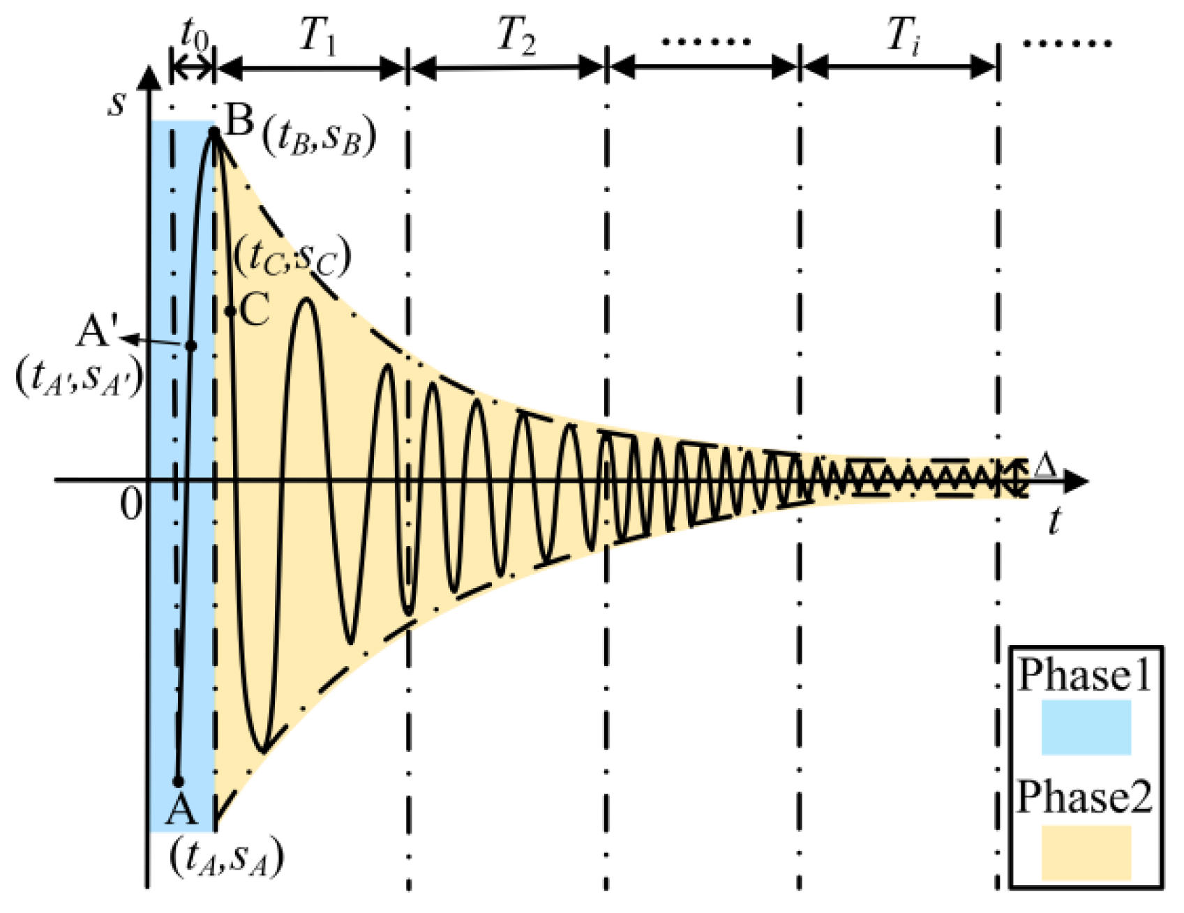
4. Improved Adaptive 2-SM Controller

In order to solve the problem of the fixed control gain for the traditional 2-SM control, a novel adaptive mechanism, based on online zero-crossing detection [43,44,45], was introduced. For the purpose of comparison, the twisting algorithm [35] was still taken as an example of 2-SM in the following. The improvement was carried out via sliding surface and control law, simultaneously.

4.1. Design of Sliding Surface

In order to improve the steady performance of the converter system, the original sliding surface in (6) was improved by introducing the integral term of the state x₁, i.e.,

$$s=c_1{x}_1+x_2+c_2{\displaystyle {\int }_0^t{x}_{1}dt}$$

(15)

where the design parameters c₁ > 0 and c₂ > 0; and the purpose of the added integral term was to eliminate the static error of the state x₁ and further improve the quality of the output voltage of the buck converters.

Furthermore, we defined a new vector w = [w₁, w₂]^T= [${\displaystyle {\int }_0^t{x}_1}dt$, x₁]^T. Therefore, by combining (4), (15) could be changed to

$$\{\begin{array}{l}{\dot{w}}_1=w_2\\ {\dot{w}}_2=-c_1{w}_2-c_2{w}_1+s\end{array}$$

(16)

Then, by substituting (16) to the first-order derivative of (15), $\dot{s}$ could be deduced as

$$\dot{s}=y_1+\mu u$$

(17)

where,

$$y_1=\left(c_1+{\beta }_2\right)s+\left(-c_1{c}_2-c_2{\beta }_4\right)w_1+\left(-c_1{}^2-c_1{\beta }_2+c_2+{\beta }_1\right)w_2+{\beta }_4\left(t\right)$$

(18)

Based on the proof of Theorem 1 and (9), we continued to calculate the derivative of (17). The derivative of the control u appeared directly on the second-order derivative of the sliding variable s like (9), i.e.,

$$\ddot{s}=y_{21}\left(w,s\right)+y_{22}\left(u\right)+y_{23}\left(t\right)+{\beta }_3\dot{u}$$

(19)

with

$$\begin{array}{ll}{y}_{21}\left(w,s\right)& =\left(-c_1{c}_2{\beta }_2-c_2{\beta }_1+c_2{\beta }_2{}^2-c_2{}^2\right)w_1+\left({\beta }_1{\beta }_2-c_1{c}_2-c_1{}^2{\beta }_2-c_1{\beta }_2{}^2\right)w_2\\ & +\left(c_2+{\beta }_1+c_1{\beta }_2+{\beta }_2{}^2\right)s\end{array}$$

(20)

$$y_{22}\left(u\right)=\left(c_1+{\beta }_2\right){\beta }_{3}u$$

(21)

$$y_{23}\left(t\right)=\left(c_1+{\beta }_2\right){\beta }_3+{\dot{\beta }}_3$$

(22)

In order to further elaborate the boundary of the parameters in (20)–(22), the variables ζ₁, ζ₂, ζ₃, ζ₄(t), Y₂₁(||w||, |s|), Y₂₂( u ), Y₂₃(t) were introduced, respectively, as

$$\{\begin{array}{l}{\zeta }_1=\max \left\{c_1,{\beta }_2\right\}\\ {\zeta }_2=\max \left\{\left|-c_1{c}_2{\beta }_2-c_2{\beta }_1+c_2{\beta }_2^2-c_1{}^2\right|,\left|{\beta }_1{\beta }_2-c_1^2{\beta }_2-c_1{\beta }_2^2-c_1{c}_2\right|\right\}\\ {\zeta }_3=\max \left\{\left|c_1{\beta }_2+{\beta }_1\right|,\left|c_2+{\beta }_2^2\right|\right\}\\ {\zeta }_4\left(t\right)=\max \left\{{\beta }_3\left(t\right),{\dot{\beta }}_3\left(t\right)\right\}\end{array}$$

(23)

$$\{\begin{array}{l}{Y}_{21}\left(\Vert w\Vert ,\left|s\right|\right)={\zeta }_2\left(\left|w_1\right|+\left|w_2\right|\right)+{\zeta }_3\left|s\right|\\ Y_{22}\left(u\right)={\zeta }_1{\beta }_{3}u\\ Y_{23}\left(t\right)={\zeta }_1{\zeta }_4\left(t\right)\end{array}$$

(24)

which were satisfied with the following inequations

$$\{\begin{array}{l}\left|y_{21}\left(w,s\right)\right|\le Y_{21}\left(\Vert w\Vert ,\left|s\right|\right)\\ \left|y_{22}\left(u\right)\right|\le Y_{22}\left(u\right)\\ \left|y_{23}\left(t\right)\right|\le Y_{23}\left(t\right)\end{array}$$

(25)

4.2. Design of Control Law

In this paper, the adaptive mechanism based on online zero-crossing detection was introduced to improve the control law of the traditional twisting algorithm [35] in (6). Its idea was based on the “switching” nature of the real (non-ideal) SM and its adaptive mechanism depended on counting the zero-crossing points of the sliding variable in a certain time interval [45], illustrated in Figure 3.

In Figure 3, the convergence process of the general control system is illustrated. Based on the adaptive mechanism of online zero-crossing detection, the trajectory was divided into two phases.

• Phase 1: Point A–Point B

In the first phase, Point A refers to the initial point of the system trajectory, while Point B refers to the first peak point satisfied with $\dot{s}=0$ for the sliding surface in (15). In Phase 1, it starts from Point A (t_A, s_A) and ends at Point B (t_B, s_B). In order to guarantee the finite convergence time t₀ = t_B − t_A, the condition $\dot{s}(t_B)=0$ should be satisfied. Therefore, the control law of the traditional twisting algorithm in (8) is changed to

$${\dot{u}}_1=-U\left(w,s,u_1,t\right)\mathrm{sgn}\left(s\right)$$

(26)

where u₁ is the control law in Phase 1, and

$$\begin{array}{ll}U\left(w,s,u_1,t\right)& =\frac{1}{{\mu }_{\beta 3\min }}\left[Y_{21}\left(\Vert w\Vert ,\left|s\right|\right)+Y_{22}\left(\left|u_1\right|\right)+Y_{23}\left(t\right)+k\right]\\ & =\frac{1}{{\mu }_{\beta 3\min }}[{\zeta }_2\left(\left|w_1\right|+\left|w_2\right|\right)+{\zeta }_3\left|s\right|+{\zeta }_1{\beta }_3\left|u_1\right|+{\zeta }_1{\zeta }_4\left(t\right)+k]\end{array}$$

(27)

where the design parameter is k > 0.

In Phase 1, attention should be paid to the existence of Point B, which was investigated in the following Theorem 2.

Theorem 2.

For the buck converter with disturbances in (4), if the sliding surface and the control law are designed as (15) and (26), the system can research to Point B in a finite time.

Proof of Theorem 2.

By substituting the control law (26) into the second-order derivative of the sliding variable in (19), there was

$$\begin{array}{ll}\ddot{s}& =y_{21}\left(w,s\right)+y_{22}\left(u_1\right)+y_{23}\left(t\right)+{\beta }_3\dot{u}\\ & =y_{21}+y_{22}+y_{23}-{\beta }_3\mathrm{sgn}\left(s\right)\frac{1}{{\mu }_{\min }}[{\zeta }_2\left(\left|w_1\right|+\left|w_2\right|\right)+{\zeta }_3\left|s\right|+{\zeta }_2\mu \left|u_1\right|+{\zeta }_1{\zeta }_4\left(t\right)+k]\\ & =y_{21}+y_{22}+y_{23}-\frac{{\beta }_3}{{\mu }_{\beta 3\min }}\left[Y_{21}+Y_{22}+Y_{23}+k\right]\mathrm{sgn}\left(s\right)\end{array}$$

(28)

For Point B, if it was satisfied with $\dot{s}(t_B)=0$, it was necessary to check the symbol of the function of $\mathrm{sgn}(s)\ddot{s}$, i.e.,

$$\begin{array}{ll}\mathrm{sgn}\left(s\right)\ddot{s}& =\mathrm{sgn}\left(s\right)\left[y_{21}+y_{22}+y_{23}-\frac{{\beta }_3}{{\mu }_{\beta 3\min }}\left(Y_{21}+Y_{22}+Y_{23}+k\right)\right]\\ & \le \mathrm{sgn}\left(s\right)\left[y_{21}+y_{22}+y_{23}\right]-\left|y_{21}\right|-\left|y_{22}\right|-\left|y_{23}\right|-k\\ & \le \left|y_{21}\right|+\left|y_{22}\right|+\left|y_{23}\right|-\left|y_{21}\right|-\left|y_{22}\right|-\left|y_{23}\right|-k\\ & \le -k<0\end{array}$$

(29)

Since $\mathrm{sgn}(s)\ddot{s}\le -k$≤ 0, it was equivalent to $s\ddot{s}\le -k\left|s\right|$, which meant the system could research to Point B in a finite time t_B. It completes the proof. □

• Phase 2: Convergence process after Point B

In this phase, the adaptive mechanism of the online zero-crossing detection would work [45]. Compared with the traditional control law in (8) with fixed control gain, its purpose was to regulate the steady error of the output voltage to the arbitrarily value Δ by time-varying control gain, i.e.,

$${\dot{u}}_2=-U_i\left[\mathrm{sgn}(s)+r_4\mathrm{sgn}(\dot{s})\right]$$

(30)

where r₄> 0 is a design parameter, U_i is an adaptive control gain determined by checking the number of the zero-crossing point in a sampling time interval T_i, i.e.,

$$U_{i+1}=\{\begin{array}{l}\max \left(U_i-{\Lambda }_{1}T,0\right)N_i\ge N^{*}\\ \min \left(U_i+{\Lambda }_{2}T,U_0\right)N_i<N^{*}\end{array}$$

(31)

where in the time interval T_i, N_i is the number of the zero-crossing points, N^* is its given value satisfied with N* ≥ 2; Λ₁ and Λ₂ are positive constants with Λ₁ < Λ₂; U₀ is the initial value of u₂ at Point B, and is as the same as the maximum value of U (w, s, u₁, t) in (27) in Phase 1, i.e.,

$$U_0=\left[Y_{21}\left({\Vert w\Vert }^{*},\left|s(t_B)\right|\right)+Y_{22}\left(u_{1\max }\right)+Y_{23}\left(t_B\right)+k\right]$$

(32)

where u_1max is the maximum value of the control u₁ in Phase 1, ||w||^* is the upper boundary of w and can be denoted from (26) as

$${\Vert w\Vert }^{*}=\underset{\left|u\right|\le u_{1\max }}{\sup }\Vert w\Vert$$

(33)

Theorem 3.

For the buck converter with disturbances in (4), if the sliding surface is designed as (15) and the adaptive control laws are designed as (30)–(33), the converter system can converge to the region described as

$$\{\begin{array}{l}\left|\dot{s}\right|\le \left[U_0+\left(1+r_4\right){\mu }_{\beta 3\max }{U}_i\right]T\\ \left|s\right|\le \left[U_0+\left(1+r_4\right){\mu }_{\beta 3\max }{U}_i\right]T^2\end{array}$$

(34)

Proof of Theorem 3.

In Phase 2, we substituted the adaptive control law u2 in (30)–(33) into the second-order derivative of the sliding variable in (18), and there was

$$\begin{array}{ll}\ddot{s}& =y_{21}+y_{22}+y_{23}+{\beta }_3\left\{-U_i\left[\mathrm{sgn}(s)+r_4\mathrm{sgn}(\dot{s})\right]\right\}\\ & \le \left|y_{21}\right|+\left|y_{22}\right|+\left|y_{23}\right|+\left(1+r_4\right){\beta }_3{U}_i\end{array}$$

(35)

From Figure 3, since Point B represented the first peak of the sliding variable s in Phase 1, it was also the maximum value in Phase 2. By combining (24), (25), (32) and (33), (35) could be further changed to

$$\begin{array}{ll}\ddot{s}& \le Y_{21}\left[\Vert w\Vert *,\left|s(t_B)\right|\right]+Y_{22}\left(u_{1\max }\right)+Y_{23}\left(t_B\right)+k+(1+r_4){\beta }_3{U}_i\\ & \le U_0+(1+r_4){\mu }_{\beta 3\max }{U}_i\end{array}$$

(36)

Furthermore, we zoomed up the interval T_i as an example to further investigate the adaptive mechanism of the online zero-crossing detection within a single sampling interval T, shown in Figure 4. For the arbitrary zero-crossing points at the moment t_i and t_j, there was s(t_i) = s(t_j) = 0, i∈[1, N_j], j∈[1, N_j], i < j. Since the given number of the zero-crossing point N^* ≥ 2, it meant there were at least two points of zero-crossing detection within a single sampling interval T. Based on Rolle’s theorem, there must exist a zero-crossing point $\dot{s}(t_{ij})=0$ with t_i < t_ij < t_j. Meanwhile, as the system converged to the equilibrium point, the smaller the oscillation amplitude of the sliding variable s was, the larger the number of the zero-crossing points. Therefore, the choice of the given number of the zero-crossing points N^* was crucial and could be determined by experiment with N^* = max{2 T f_i + 1}(j = 1,2,3,...), where f_i = N_i/T.

Based on Rolle’s theorem, there must exist a zero-crossing point $\dot{s}(t_{ij})=0$ with t_i < t_ij < t_j. Meanwhile, based on the Lagrange mean value theorem, there must exist a moment t_ij′, which is located between t and t_ij and from (35), this was satisfied with

$$\left|\ddot{s}\left({t^{\prime }}_{ij}\right)\right|=\left|\frac{\dot{s}\left(t\right)-\dot{s}\left(t_{ij}\right)}{t-t_{ij}}\right|\le \left[U_0+\left(1+r_4\right){\mu }_{\beta 3\max }{U}_i\right]$$

(37)

where t is an arbitrary moment except t_ij in the sampling interval T_i, and is satisfied with |t – t_ij | < T. It completed the proof. □

5. Simulations and Experiments

In order to validate the improved twisting algorithm with the adaptive mechanism of online zero-crossing detection, as well as to show its unified robustness in converter systems with multi-disturbances, we compared it with the traditional 1-SM and the twisting algorithm, simultaneously, where the commonly used LSM was chosen as an example of 1-SM. For the convenience of analysis and comparison, they are abbreviated as “1-SMC”, “2T-SMC” and “2AT-SMC”, respectively.

For the buck converter in Figure 1, its circuit parameters are listed in

Table 1. Circuit parameters of the buck converter.

Symbols	Parameters	Values
L	Inductance	1 mH
C	Capacitance	1000 μF
R	Load resistance	10 Ω
Vref	the Reference voltage	5 V
E	Input DC voltage	10 V

. In the following, we comprehensively compared the three control approaches in conditions with/without disturbances by simulations and experiments.

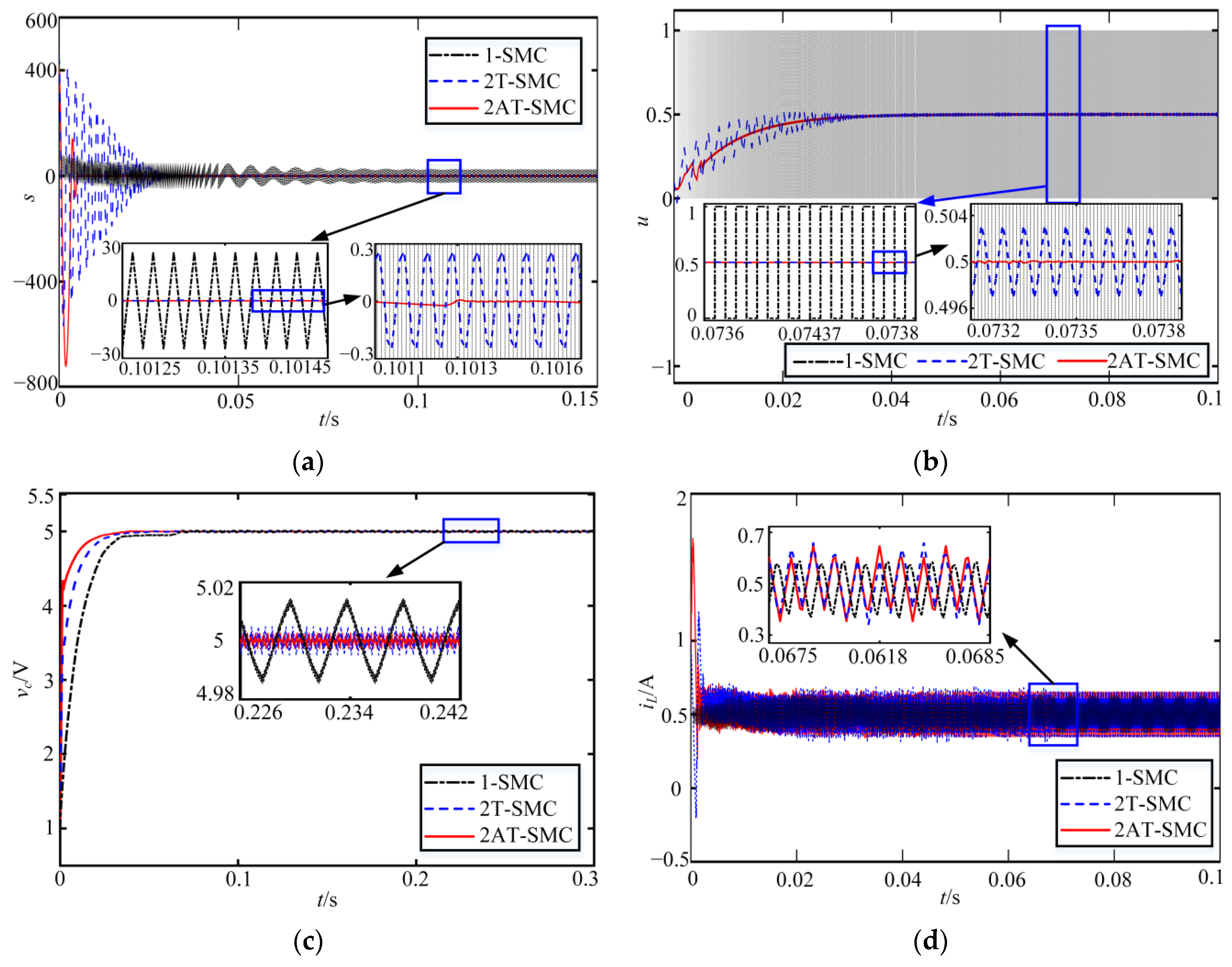
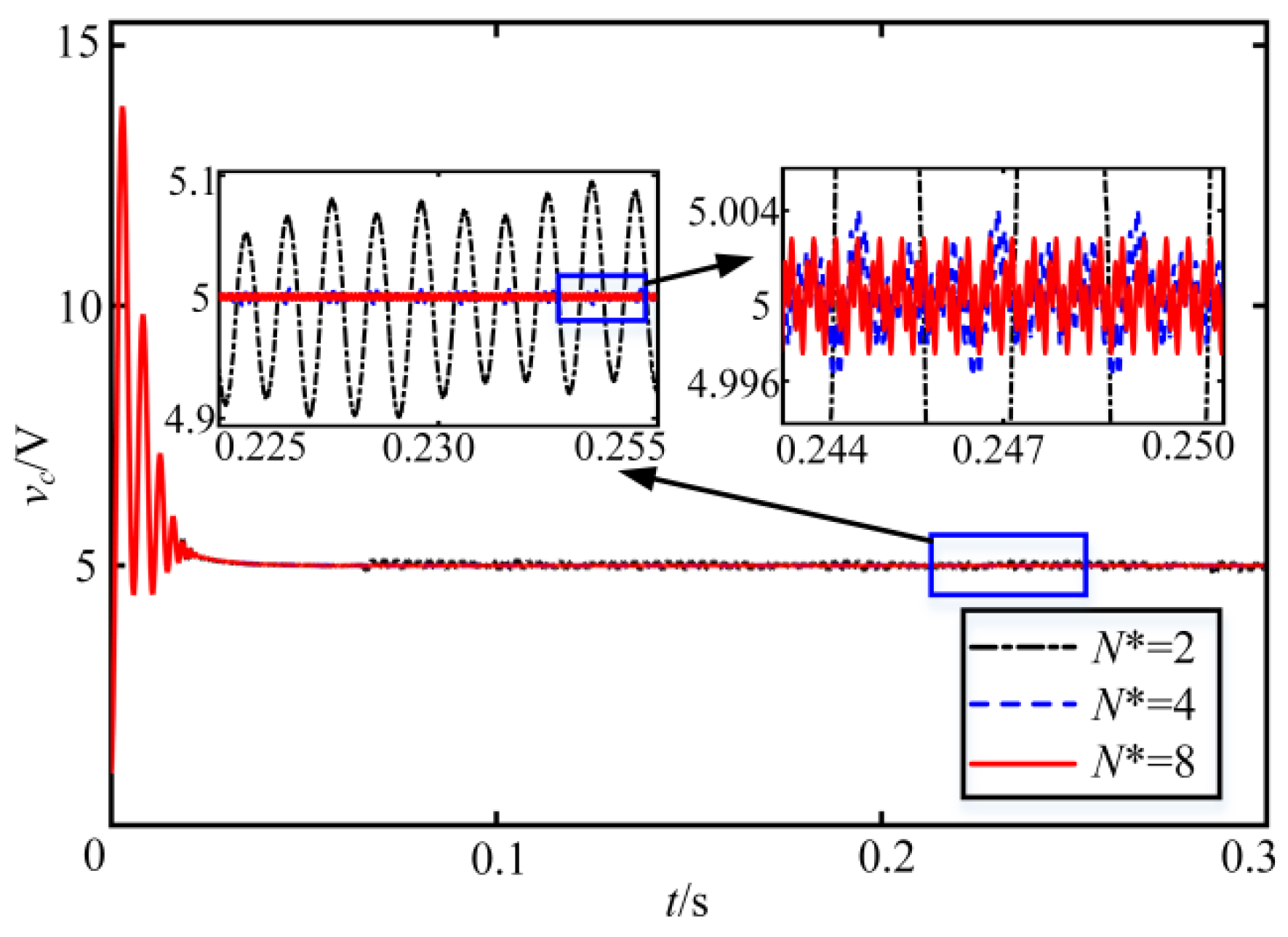
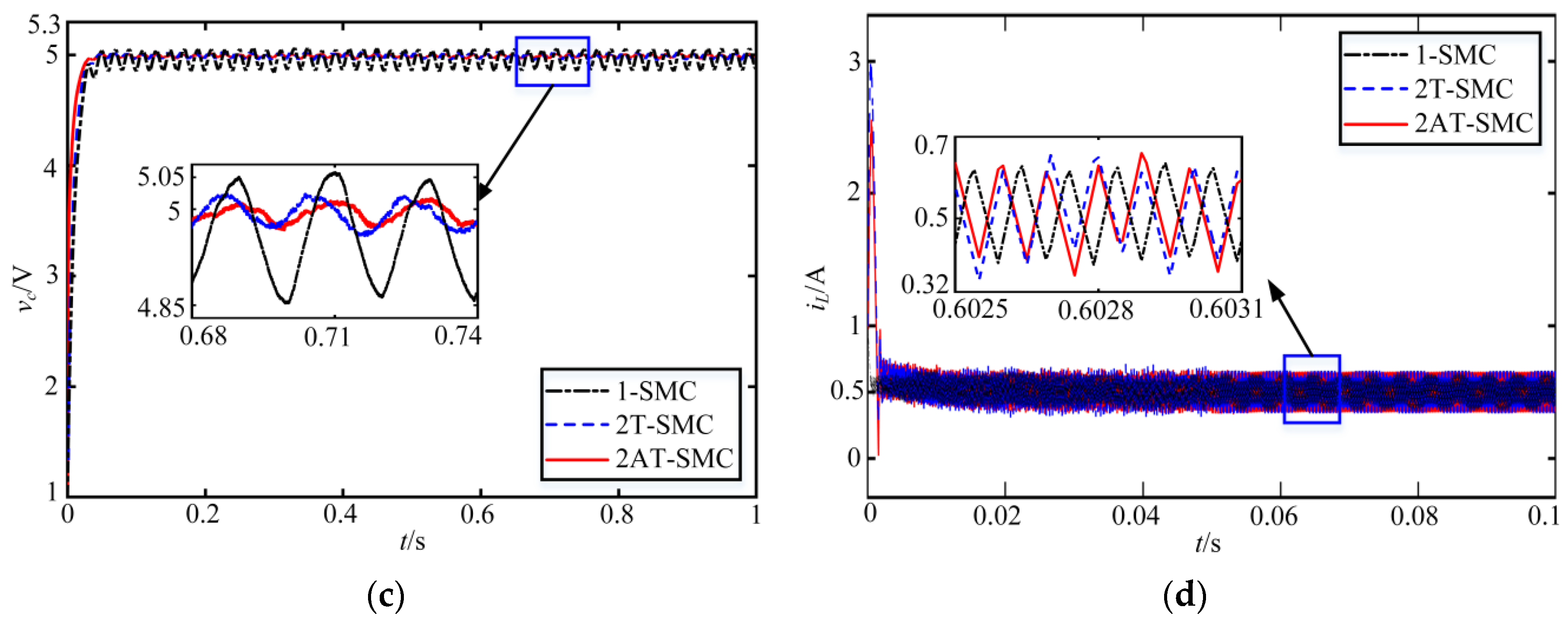
5.1. Simulation Results and Analysis

The design of SM controllers includes two parts, i.e., a sliding surface and a control law. For 1-SMC in (6) and (7), 2T-SMC in (6) and (8), 2AT-SMC in (15), (26) and (30), the three comparative controllers were designed respectively as

• SMC

$$\{\begin{array}{l}s=110x_1+x_2\\ u=-\frac{1}{2}\left[\mathrm{sgn}\left(s\right)-1\right]\end{array}$$

(38)

• 2T-SMC

$$\{\begin{array}{l}s=110x_1+x_2\\ \dot{u}=-320\mathrm{sgn}(s)-300\mathrm{sgn}(\dot{s})\end{array}$$

(39)

• 2AT-SMC

$$\{\begin{array}{l}s=110x_1+x_2+0.1{\displaystyle {\int }_0^t{x}_{1}dt}\\ {\dot{u}}_1=-U\left(w,s,u_1,t\right)\mathrm{sgn}\left(s\right)\\ {\dot{u}}_2=-U_i\left[\mathrm{sgn}(s)+220\mathrm{sgn}(\dot{s})\right]\\ U_{i+1}=\{\begin{array}{l}\max \left(U_i-{\Lambda }_{1}T,0\right)\hspace{1em}{N}_i\ge N^{*}\\ \min \left(U_i+{\Lambda }_{2}T,U_0\right)\hspace{1em}{N}_i<N^{*}\end{array}\end{array}$$

(40)

where the sampling time T = 40 μs, the given number of the zero-crossing points N* = 8, Λ₁ = 12, Λ₂ = 24, defined in (27) and (31), respectively.

In order to compare the control performances of the above three control approaches, simulations were carried out in the following two cases, i.e., rated working condition and that with multi-disturbances.

• Case 1: Rated working condition.

In the case of rated working condition, the simulation comparisons of the three controllers in (38)–(40) are given in Figure 5 and Figure 6 and

Table 2. Performance comparisons of the buck converter system in rated working case.

SM Controller	Output Voltage vc		Inductor Current iL
	Steady Error (mV)	Convergence Time (s)	Steady Error (A)	Convergence Time (s)
1-SMC	15.13	0.055	0.098	0.057
2T-SMC	6.09	0.042	0.113	0.043
2AT-SMC	3.01	0.031	0.101	0.032

, respectively.

When the system worked in rated working condition, Figure 5a shows the convergence process of the sliding variable s. It can be seen that, the three controllers could all force the system to converge to the equilibrium point, but 1-SMC suffered from large oscillation amplitudes, especially at the beginning. Furthermore, we zoomed up on the local comparison diagram of 2T-SMC and 2AT-SMC. Obviously, the steady performance of 2AT-SMC was better, due to the introduction of the adaptive mechanism, where the control law u, the output voltage v_c and inductor current i_L were the concerned performance indices for the buck converters. For the control law u in Figure 5b, we could see that the chattering phenomenon was serious for 1-SM, due to the switching nonlinearity of (7) [22,23,24]. Since the reference value of the output voltage v_c was 5 V, the input DC voltage was 10 V, and the duty cycle of the converter was 0.5. By zooming up the local comparison of 2T-SMC and 2AT-SMC, the control signals, u, were in the neighborhood of 0.5, due to the integral operation of 2-SM in (8), (26) and (30) [33,34,38]; meanwhile, for the latter, its performance was smooth and better, which was related to the varying control gain imposed by the adaptive mechanism of the online zero-crossing detection. For the output voltage v_c and inductor current i_L in Figure 5c,d, the corresponding performances are given in Table 2. Obviously, the control performance of 2AT-SMC was the best, due to the improvement of the adaptive mechanism. The steady error of the output voltage v_c was 3.01 mV, the convergence time was 0.031 s; while the corresponding values of the inductor current i_L were 0.101 A and 0.032 s, which validated this paper.

In order to further test the effectiveness of the adaptive mechanism in (31), the given number of the zero-crossing points N* was chosen as 2, 4, 8, and the comparative simulations are shown in Figure 6. Here we took the output voltage v_c as an example, and we could see the steady errors of the three cases listed as 48.01 mV, 6.23 mV and 3.01 mV, respectively. It meant that, the smaller N* was, the bigger the steady error was, which was in accordance with the proof in Theorem 3. It also validated the effectiveness of the proposed adaptive mechanism, based on the online zero-crossing detection [43,44,45].

• Case 2: The working condition with multi-disturbances.

In practice, there generally exist multi-disturbances, and seldom is there only one type. This was also the reason that we considered the possible parameter perturbations and external disturbances of the buck converters in (5). In the following, we simulated these multi-disturbances by sine function in

Table 3. Defined the possible disturbances in the buck converter system.

Disturbance Source	Disturbance Modle
∆L	0.1sin(100πt) (mH)
∆C	100sin(100πt) (μF)
∆R	sin(100πt) (Ω)
∆E	sin(100πt) (V)
∆Vref	0.5sin(100πt) (V)
d1(t)	0.04sin(4 × 107πt) (V)
d2(t)	0.04sin(4 × 107πt) (V)

. Under the control of the three kinds of SM in (38)–(40), the comparative simulations of the system with multi-disturbances are given in Figure 7 and

Table 4. Comparison of voltage and current in multi-disturbed working case.

SMC Algorithm	Output Voltage vc		Inductor Current iL
	Steady Error (mV)	Convergence Time (s)	Steady Error (A)	Convergence Time (s)
1-SMC	155.13	0.069	0.121	0.071
2T-SMC	51.26	0.050	0.233	0.057
2AT-SMC	25.41	0.039	0.135	0.040

, respectively.

When the buck converter system worked in disturbing condition, the simulations are given in Figure 7 and similar conclusions could be obtained in Figure 5 in rated working condition, i.e., the control performance of 2AT-SMC was the best, then 2T-SMC and the last was 1-SMC. Regardless of the possible parameter perturbations and external disturbances in Table 3, the sliding variable s under the three SM approaches could converge to the equilibrium point, simultaneously, seen in Figure 5a, due to the inherent robustness of SM. For the control law in Figure 5b, the comparative simulations also validated the capability of 2-SM over 1-SM in chattering elimination, and the duty cycle of 2T-SMC and 2AT-SMC still maintained around 0.5, but the latter was better due to the varying control gain produced by the adaptive mechanism. The output voltage v_c and the inductor current i_L are illustrated in Figure 5c,d, and the corresponding steady error and convergence time are given in Table 4. By combining Table 2 and Table 4, the control performances of both were the best under the control of 2AT-SMC. Taking the output voltage v_c as an example, the steady errors of the buck converter in rated working condition increased from 3.01 mV to 25.41 mV in the disturbing case, while for the convergence time, it increased from 0.031 s to 0.039 s, which was due to the existence of parameter perturbations and external disturbances. Therefore, the simulations validated the proposed 2AT-SMC.

5.2. Experiment

In the following, we further tested the control performance and adaptation mechanism of the proposed 2AT-SMC by experiment. In Figure 8a, the experiment platform, based on DSpace 1006 was given, where the sampling time was 0.5 ms and the PWM frequency 1000 Hz; and Figure 8b is the hard ware of the buck converter.

In the experiment, we considered the possible parameter perturbations and external disturbances of the buck converters in Table 1. Specifically, the parameter vibrations of the inductor L and capacitor C were in accordance with the practical elements, i.e., 0 < ∆L < 0.1 mH and 0 < ∆C < 10⁻⁴ F [46,47]; and for the other disturbances in Table 1, we assumed:

• The input voltage E increased from 10 V to 11 V at t = 1 s, and then reduced to 10 V at t = 2 s, i.e., ∆E = 1 V;
• The reference voltage V_ref increased from 5 V to 5.5 V at t = 3 s, and then reduced to 5 V at t = 4 s, i.e., ∆V_ref = 0.5 V;
• The load resistor R increased from 10 Ω to 11 Ω at t = 5 s, and then reduced to 10Ω at t = 6 s, i.e., ∆R = 1 Ω.
• The above three disturbances existed simultaneously at t = 7 s, and then disappeared at t = 8 s.

Based on the above four cases, we used the time-varying disturbances to simulate the individual, several or all disturbances in practice [2]. The experiment results under the control of 1-SMC, 2T-SMC and 2AT-SMC are compared in Figure 9,

Table 5. Experimental comparisons of steady error.

Disturbance Source	SM Algorithms
	1-SMC		2T-SMC		2AT-SMC
	vc (mV)	iL (A)	vc (mV)	iL (A)	vc (mV)	iL (A)
-	314.05	0.407	152.42	0.396	114.23	0.367
∆E(1 s–2 s)	367.41	0.422	171.40	0.412	124.11	0.384
∆Vref (3 s–4 s)	322.32	0.437	153.32	0.427	116.33	0.401
∆R(5 s–6 s)	415.34	0.385	196.13	0.366	152.24	0.337
[∆E + ∆Vref + ∆R](7 s–8 s)	454.38	0.374	234.03	0.358	183.03	0.327

and

Table 6. Experimental comparisons of response time.

Disturbance Source	SM Algorithms
	1-SMC		2T-SMC		2AT-SMC
	t(vc) (s)	t(iL) (s)	t(vc) (s)	t(iL) (s)	t(vc) (s)	t(iL) (s)
∆E(1 s–2 s)	0.115	0.117	0.094	0.102	0.082	0.089
∆Vref (3 s–4 s)	0.099	0.104	0.085	0.093	0.078	0.085
∆R(5 s–6 s)	0.118	0.121	0.102	0.109	0.087	0.099
[∆E + ∆Vref + ∆R](7 s–8 s)	0.132	0.135	0.112	0.118	0.089	0.105

.

In Table 5 and Table 6,the performance comparisons of the steady error and response time of the output voltage v_c and inductor current i_L, respectively, are shown and they are in accordance with the time-varying information in Figure 9. The same conclusion can be obtained in Figure 6 and Figure 7, Table 2 and Table 4 in the simulation, i.e., the control performances under the control of 2AT-SMC was the best among the three SM algorithms. Meanwhile, the three SM algorithms were all robust against the parameter perturbations and external disturbances of the buck converters. Attention should be paid to the fact that the unified robustness of 1-SMC was due to the two-value of the control u in (7) and (38), where the detailed explanation can be seen in [2]; while for 2T-SMC and 2AT-SMC, their unified robustness was due to the twisting algorithm itself [35], which only needed the boundary information of these multi-disturbances. It was also the reason for the fact that the twisting algorithm is widely used in practical systems, as well as the reason that we chose it as the example of 2-SM.

Therefore, the comparative simulations and experiments in rated working condition and in disturbing condition could all validate the proposed 2AT-SMC with better robustness and control performances due to the adaptive mechanism of online zero-crossing detection. Meanwhile, it was significant for the robust control of power converters with disturbances.

6. Conclusions

In this paper, a novel adaptive 2-SM was proposed for the robust control of buck converters with multi-disturbances. Compared with the traditional 1-SM and 2-SM, control continuity and variable control gain could be achieved due to the adaptive mechanism of online zero-crossing detection, so that the inherent problems of chattering and fixed control gain could be effectively solved. Meanwhile, the variations of input and reference output voltage, parameter uncertainties of load resistor, inductor, and capacitor, and time-varying external disturbances were all considered in the modeling of buck converters. The application of the twisting algorithm with 2-SM could provide a unified robustness for buck converters, whether individual, several or all disturbances existed in practice. Innovatively, the robust stability of the system was investigated in phase plane; while the adaptive mechanism of online zero-crossing detection was investigated in accordance with the system convergence. Comparative simulations and experiments with multiple working conditions validated the advantages of this paper as offering better robustness and control performances.

References

1. Wang, Y.; Niu, Z.; Yang, M.; Sun, L.; Zhang, W. Stability of Sliding Mode Controlled Buck Converters with Unmodelled Dynamics of Circuit Elements and Hall Sensor. IET Power Electron. 2021, 14, 602–613. [Google Scholar] [CrossRef]
2. Wang, Y.; Ge, Y.; Zhang, P.; Duan, G. Unified Approach for Robust Stability Analysis of Buck Converters with Discrete-Time Sliding Mode Control. Math. Probl. Eng. 2021, 2021, 5527047. [Google Scholar] [CrossRef]
3. Chen, C.H.; Cheng, P.G.; Xie, M.J. Current Sharing of Paralleled DC-DC Converters Using GA-based PID Controllers. Expert Syst. Appl. 2010, 14, 733–740. [Google Scholar] [CrossRef]
4. Olm, J.M.; Biel, D. Linear Robust Output Regulation in a Class of Switched Power Converters. Math. Probl. Eng. 2010, 2010, 724531. [Google Scholar] [CrossRef]
5. Chen, G.; Chen, L.; Deng, Y. Single Coupled-inductor Dual Output Soft-switching DC–DC Converters with Improvedcross-regulation and Reduced Components. IET Power Electron. 2017, 10, 1665–1678. [Google Scholar] [CrossRef] [Green Version]
6. Cha, H.R.; Kim, Y.; Park, K.H.; Choi, Y.J. Modeling and Control of Double-Sided LCC Compensation Topology with Semi-Bridgeless Active Rectifier for Inductive Power Transfer System. Energies 2019, 12, 3921. [Google Scholar] [CrossRef] [Green Version]
7. Tan, S.; Lai, C.D.; Cheung, K.H.; Tse, C.K. General Design Issues of Sliding-mode Controllers in DC–DC Converters. IEEE Trans. Power Electron. 2005, 20, 425–437. [Google Scholar] [CrossRef] [Green Version]
8. Ahmad, S.; Ali, A. Active Disturbance Rejection Control of DC-DC Boost Converter: A Review with Modifications for Improved Performance. IET Power Electron. 2019, 12, 2095–2107. [Google Scholar] [CrossRef]
9. Zhao, Y.; Qiao, W.; Ha, D. A Sliding-Mode Duty-Ratio Controller for DC/DC Buck Converters With Constant Power Loads. IEEE Trans. Ind. Appl. 2014, 50, 1448–1458. [Google Scholar] [CrossRef] [Green Version]
10. Gautam, A.R.; Gourav, K.; Guerrero, J.M.; Fulwani, D.M. Ripple Mitigation with Improved Line-Load Transients Response in a Two-Stage DC-DC-AC Converter: Adaptive SMC Approach. IEEE Trans. Ind. Electron. 2018, 65, 3125–3135. [Google Scholar] [CrossRef]
11. Mattavelli, P.; Rossetto, L.; Spiazzi, G.; Tenti, P. General-purpose fuzzy controller for DC-DC converters. IEEE Trans. Power Electron. 1997, 12, 79–86. [Google Scholar] [CrossRef] [Green Version]
12. Babes, B.; Mekhilef, S.; Boutaghane, A.; Rahmani, L. Fuzzy Approximation-Based Fractional-Order Nonsingular Terminal Sliding Mode Controller for DC-DC Buck Converters. IEEE Trans. Power Electron. 2022, 37, 2749–2760. [Google Scholar] [CrossRef]
13. Rubaai, A.; Ofoli, A.R.; Burge, L.; Garuba, M. Hardware Implementation of an Adaptive Network-based Fuzzy Controller for DC-DC Converters. IEEE Trans. Ind. Appl. 2005, 41, 1557–1565. [Google Scholar] [CrossRef]
14. Rojas-Dueñas, G.; Riba, J.R.; Moreno-Eguilaz, M. Black-Box Modeling of DC-DC Converters Based on Wavelet Convolutional Neural Networks. IEEE Trans. Inst. Meas. 2021, 70, 2005609. [Google Scholar] [CrossRef]
15. Bastos, R.F.; Aguiar, C.R.; Gonçalves, A.F.Q.; Machado, R.Q. An Intelligent Control System Used to Improve Energy Production from Alternative Sources With DC-DC Integration. IEEE Trans. Smart Grid. 2014, 5, 2486–2495. [Google Scholar] [CrossRef]
16. Khooban, M.H.; Gheisarnejad, M.; Farsizadeh, H.; Masoudian, A.; Boudjadar, J. A New Intelligent Hybrid Control Approach for DC-DC Converters in Zero-Emission Ferry Ships. IEEE Trans. Power Electron. 2020, 35, 5832–5841. [Google Scholar] [CrossRef]
17. Chanjira, P.; Tunyasrirut, S. Intelligent Control Using Metaheuristic Optimization for Buck-Boost Converter. J. Eng. 2020, 2020, 5462871. [Google Scholar] [CrossRef]
18. Fang, J.S.; Tsai, S.H.; Yan, J.J.; Chen, P.L.; Guo, S.M. Realization of DC-DC Buck Converter Based on Hybrid H2 Model Following Control. IEEE Trans. Ind. Electron. 2022, 69, 1782–1790. [Google Scholar] [CrossRef]
19. Wang, Y.; Huang, P.; Ji, S.; Dai, M. Improved Linear Sliding Mode Controller of Buck Converters through Adding Terminal Sliding Mode. In Proceedings of the 11th Asian Control Conference (ASCC), Gold Coast, Australia, 17–20 December 2017; pp. 682–686. [Google Scholar]
20. Amin, M.S.; Babaei, E. Robust Nonlinear Controller Based on Control Lyapunov Function and Terminal Sliding Mode for Buck Converter. Int. J. Numer. Model. Electron. Netw. Device Fields 2016, 29, 1055–1069. [Google Scholar]
21. Hasan, K. Non-singular Terminal Sliding-mode Control of DC-DC Buck Converters. Control Eng. Pract. 2013, 21, 321–332. [Google Scholar]
22. Elnady, A. Newly Developed First-order Sliding Mode of Power and Voltage Control for the Diode-clamped Multilevel Inverter. Int. J. Power Energy Syst. 2017, 37, 150–163. [Google Scholar] [CrossRef]
23. Xiong, X.G.; Chen, H.; Liu, Z.; Yamamoto, M.; Lou, Y. Implicit Discrete-Time Adaptive First-Order Sliding Mode Control with Predefined Convergence Time. IEEE Trans. Circuits Syst. II-Express Briefs 2021, 68, 3562–3566. [Google Scholar] [CrossRef]
24. Sivaramakrishnan, S.; Tangirala, A.K.; Chidambaram, M. Sliding Mode Controller for Unstable Systems. Chem. Biochem. Eng. Q. 2008, 22, 41–47. [Google Scholar]
25. Boiko, I.; Fridman, L. Analysis of Chattering in Continuous Sliding-mode Controllers. IEEE Trans. Autom. Control 2005, 50, 1442–1446. [Google Scholar] [CrossRef] [Green Version]
26. Li, M.; Liu, C. Sliding Mode Control of a New Chaotic System. Chin. Phys. B 2010, 10, 148–150. [Google Scholar]
27. Ma, H.; Wu, J.; Xiong, Z. Active Chatter Control in Turning Processes with Input Constraint. Int. J. Adv. Manuf. Technol. 2020, 108, 3737–3751. [Google Scholar] [CrossRef]
28. Hua, S.; Wang, X.; Zhu, Y. Sliding-mode Control for a Rolling-missile with Input Constraints. J. Syst. Eng. Electron. 2020, 31, 1041–1050. [Google Scholar]
29. Zong, Q.; Zhao, Z.; Zhang, J. Higher Order Sliding Mode Control with Self-tuning Law Based on Integral Sliding Mode. IET Control Theory Appl. 2010, 4, 1282–1289. [Google Scholar] [CrossRef]
30. Mahjoub, S.; Ayadi, M.; Derbel, N. Comparative Study of Smart Energy Management Control Strategies for Hybrid Renewable System Based Dual Input-single Output DC-DC Converter. J. Electr. Syst. 2020, 16, 218–234. [Google Scholar]
31. Farhoud, A.; Erfanian, A. Fully Automatic Control of Paraplegic FES Pedaling Using Higher-Order Sliding Mode and Fuzzy Logic Control. IEEE Trans. Neural Syst. Rehabil. Eng. 2014, 22, 533–542. [Google Scholar] [CrossRef]
32. Djilali, L.; Badillo-Olvera, A.; Yuliana Rios, Y.; López-Beltrán, H.; Saihi, L. Neural High Order Sliding Mode Control for Doubly Fed Induction Generator based Wind Turbines. IEEE Latin Am. Trans. 2022, 20, 223–232. [Google Scholar] [CrossRef]
33. Levant, A. Principles of 2-sliding Mode Design. Automatica 2007, 43, 576–586. [Google Scholar] [CrossRef] [Green Version]
34. Ding, S.; Wang, J.; Zheng, W. Second-Order Sliding Mode Control for Nonlinear Uncertain Systems Bounded by Positive Functions. IEEE Trans. Ind. Electron 2015, 62, 5899–5909. [Google Scholar] [CrossRef]
35. Rakht Ala, S.M.; Yasoubi, M.; HosseinNia, H. Design of Second Order Sliding Mode and Sliding Mode Algorithms: A Practical Insight to DC-DC Buck Converter. IEEE-CAA J. Automatica Sin. 2017, 4, 483–497. [Google Scholar] [CrossRef] [Green Version]
36. Lazar, M.; Heemels, W.P.M.H.; Roset, B.J.P.; van den Bosch, P.P.J. Input-to-state Stabilizing Sub-optimal NMPC with an Application to DC–DC Converters. Int. J. Robust Nonlinear Control 2008, 18, 890–904. [Google Scholar] [CrossRef]
37. Rakhtala, S.M.; Casavola, A. Real-Time Voltage Control Based on a Cascaded Super Twisting Algorithm Structure for DC–DC Converters. IEEE Trans. Ind. Electron 2022, 69, 633–641. [Google Scholar] [CrossRef]
38. Singh, S.; Srivastava, P.; Janardhanan, S. Adaptive Higher Order Sliding Mode Control for Nonlinear Uncertain Systems. In Proceedings of the 5th IFAC Conference on Advances in Control and Optimization of Dynamical Systems (ACODS), Hyderabad, India, 18–22 February 2018; pp. 341–346. [Google Scholar]
39. Liang, D.; Li, J.; Qu, R.; Kong, W. Adaptive Second-order Sliding-Mode Observer for PMSM Sensorless Control Considering VSI Nonlinearity. IEEE Trans. Power Electron. 2018, 33, 8994–9004. [Google Scholar] [CrossRef]
40. Thanh, H.L.N.; Hong, S.K. Quadcopter Robust Adaptive Second-Order Sliding Mode Control Based on PID Sliding Surface. IEEE Access 2018, 6, 66850–66860. [Google Scholar] [CrossRef]
41. Qiao, L.; Zhang, W. Adaptive Second-Order Fast Nonsingular Terminal Sliding Mode Tracking Control for Fully Actuated Autonomous Underwater Vehicles. IEEE J. Ocean Eng. 2019, 44, 363–385. [Google Scholar] [CrossRef]
42. Shen, X.; Liu, J.; Alcaide, A.M.; Yin, Y.; Leon, J.I.; Sergio, V.; Franquelo, L.G. Adaptive Second-Order Sliding Mode Control for Grid-Connected NPC Converters with Enhanced Disturbance Rejection. IEEE Trans. Power Electron. 2022, 37, 206–220. [Google Scholar] [CrossRef]
43. Mei, K.; Ding, S.; Zheng, W. Fuzzy Adaptive SOSM Based Control of a Type of Nonlinear System. IEEE Trans. Circuits Syst. II-Express Briefs 2022, 69, 1342–1346. [Google Scholar] [CrossRef]
44. Li, S.; Fei, A.J. Adaptive Second-Order Sliding Mode Fuzzy Control Based on Linear Feedback Strategy for Three-Phase Active Power Filter. IEEE Access 2018, 6, 72992–73000. [Google Scholar] [CrossRef]
45. Carolina, A.E.; Alessandro, P.; Paul, P.; Elio, U. Receding Horizon Adaptive Second-Order Sliding Mode Control for Doubly-Fed Induction Generator Based Wind Turbine. IEEE Trans. Control Syst. Technol. 2017, 25, 73–84. [Google Scholar]
46. Wong, O.; Wong, H.; Tam, W.; Kok, C. Parasitic Capacitance Effect on the Performance of Two-phase Switched-capacitor DC–DC Converters. IET Power Electron. 2015, 8, 1195–1208. [Google Scholar] [CrossRef]
47. Rudziński, A. Modelling of Battery-powered Boost DC-DC Power LED Driver with Parasitics by Multivariate Power Series Expansion. Int. J. Circuit Theory Appl. 2015, 43, 1197–1208. [Google Scholar] [CrossRef]
Figure 1. Structure diagram of SM controlled buck converters.
Energies 15 05139 g001
Figure 2. Convergence trajectory of the converter system under the twisting controller.
Energies 15 05139 g002
Figure 3. Adaptive mechanism of the online zero-crossing detection.
Energies 15 05139 g003
Figure 4. Online zero-crossing detection in a sampling interval.
Energies 15 05139 g004
Figure 5. Comparative simulations in rated working condition: (a) Sliding variable s; (b) Control law u; (c) Output voltage vc; (d) Inductor current iL.
Energies 15 05139 g005
Figure 6. Comparative simulations with different N*.
Energies 15 05139 g006
Figure 7. Comparative simulations in disturbing condition: (a) Sliding variable s; (b) Control law u; (c) Output voltage vc; (d) Inductor current iL.
Energies 15 05139 g007aEnergies 15 05139 g007b
Figure 8. DSpace experiment platform of the buck converter system: (a) Buck converter control system; (b) Hardware of buck converter.
Energies 15 05139 g008
Figure 9. Comparative experimental results: (a) Output voltage vc; (b) Inductor current iL; (c) Control law u.
Energies 15 05139 g009aEnergies 15 05139 g009b