A Margin Design Method Based on the SPAN in Electricity Futures Market Considering the Risk of Power Factor

Abstract

On-grid integration of renewable energy, also called “green power”, is attracting more and more attention nowadays. Green power futures can be effective in increasing returns to suppliers and increasing market liquidity. However, compared to traditional futures, green power feed-in tariffs may be subject to integrity problems due to lower power factors; therefore, existing margin calculation methods for the futures market are no longer applicable. A SPAN-based margin calculation method that considers the power factor risk is proposed in this paper. The method provides the classification policies of the green power futures, based on the historical power factors of green power suppliers, and allows the margin amount to be adjusted as per the classification. To verify the effectiveness of the proposed method, empirical validation is presented by applying actual transaction data. Results prove that the proposed method can reduce the margin amount while covering the risk effectively.

1. Introduction

Renewable energy-based “green power” has drawn increasing attention in recent times, as governments and investors have become increasingly concerned about fewer reserves and the price volatility of fossil fuels [1]. Encouraging the production of “green power” and increasing the predictability of its price will effectively mitigate the threat of fossil fuel shortage to economic development and improve the stability of energy supplements [2]. As per experience and practices, futures markets can enhance the liquidity and price stability of commodity trading. The inclusion of “green power” as an electricity commodity in the futures market by entering futures contracts could help operators guarantee the returns when electricity prices inevitably fluctuate, thus encouraging them to participate in green power futures trading and increase green power production, thus increasing the liquidity of the electricity market [3]. However, unlike traditional commodity futures represented by crude oil and cotton, as a kind of electricity future, green power futures suffer from a power factor problem [4]. When the factor is low, there is a large difference between the units of futures contracts and the actual electricity traded on the grid, thus increasing the risk for investors [5,6].

In addition, the low power factor will also have an impact on the delivery method of electricity futures. Futures trading methods usually include physical delivery and cash settlement [7]. Traders using physical delivery are usually on the short side; their role is mostly that of commodity companies with spot inventories that can sell the spot commodities they own at a determined price and realize profits; traders using cash settlement are usually on the long side and are considered speculators who push up futures prices through excess position orders over deliverable commodities to realize speculative profits [8]. In the early days of traditional electricity futures trading with physical delivery, the mismatch between futures trading volume and physical delivery volume could not be improved due to chronically low power factors, and the North American electricity market converted electricity futures contracts into pure cash settlement in the early 20th century [9]. Although the cash settlement of power futures can avoid the delivery risk, the long-term use of non-physical delivery of power futures contracts will degenerate into a purely financial speculative tool in the process of the long-short game, losing the role of guiding the expected future prices of power supply enterprises, raising operating costs, and compressing profits [10].

Therefore, it is essential for the green power futures market to design reasonable policies to reduce trading risks and increase commodity liquidity. Imposition of margin requirements is a common method used to reduce the risk of futures trading [11]. Margin is a certain amount of money that a trader must deposit to avoid default when trading futures. As a guarantee of performance on futures contracts, the margin is an important component of not only risk control in futures trading but also cost control in futures trading. It can be adjusted to influence the “leverage effect” of the futures market and the efficiency of the use of funds [12]. The amount of margin usually plays an important role in the trading conditions of the futures market. In general, lower margins do not ensure trader qualification, which affects the efficiency of market trading and may not provide effective risk warnings to sellers [13]. In contrast, higher margin requirements reduce the incentive to trade [14]; furthermore, investors affected by high margins tend to preferentially reduce their leverage to hedge their risk [15].

There are various methods of calculating margins based on risk scenarios, among which the most widely used is the SPAN (Standard Portfolio Analysis of Risk) system. This system is a portfolio-based margin calculation and risk assessment system that uses multiple indicators to estimate the maximum expected loss that could occur in a day for a portfolio of assets under market risk, and uses this loss value as the amount to calculate the margin [16]. The SPAN system can measure all risks of a portfolio of derivatives such as futures or options on a daily basis and can also measure cross-month and cross-commodity risks, covering trading risk while maximizing the elimination of inter-contract margins, improving the efficiency of traders’ capital utilization and reducing transaction costs [17]. However, the traditional SPAN system suffers from the problems of cumbersomeness and opacity. After decades of development, it requires hundreds of parameter values to be reset every day, which needs the support of huge computational power [18]. Moreover, although the SPAN system applied to the existing electricity futures market takes into account the short term–rapid–extreme price changes in futures contracts and the risks associated with delivery defaults, such risks are usually deliberately underestimated in the actual implementation due to the extremely small probability of these two changes occurring [19]. However, for green power futures, the probability of the occurrence of the aforementioned risks arising from weather and low power factor will substantially increase, especially the delivery defaults [20,21]. Therefore, the existing SPAN-based margin calculation method does not apply to the green power futures market.

For SPAN systems, the accuracy of the system parameter settings has a significant impact on the margin. The price volatility scan risk value, referring to the maximum range within which the price of a futures contract will move in one trading day, becomes a particularly important parameter in the SPAN system as the first step in margin calculation. The value at risk (VaR) measurement as a parameter setting of SPAN systems is one of the most widely used methods. It has been found that VaR modelling is partially explicable for the volatility clustering risk of the Nordic power futures [22]. A simplified algorithm based on Schwartz and Smith’s multifactor model has also proven itself as a measure of VaR in energy futures such as crude oil, electricity, and natural gas [23]. The conditional value of risk (CVaR) method has also been used to capture the risk in the tail distribution of power futures price fluctuations [24]. From the literature, it is obvious that risks captured from electricity futures contract price changes are contained in risk assessment while calculating the margin requirement. However, it is not enough to cover all the risks in the whole trading process. Few studies have incorporated risk factors other than price fluctuations, such as risk assessment at delivery, into margin calculations, and even the SPAN system does not do this. However, for the particularity of electricity futures, the delivery risk is indispensable and should be included in the margin calculation—this is the purpose of this paper.

In order to promote green power futures trading and reduce the trading risk in the green power futures market, an analysis and design of a margin requirements calculation method considering the power factor for electricity power futures based on SPAN is proposed in this paper. The method presents a rating principle for electricity power futures contracts based on the power factor affecting the delivery of electricity power futures, and then proposes a scheme to calculate price volatility risk based on the value at risk (VaR) based on the SPAN system. Finally, different levels of electricity futures are proposed to calculate the delivery risk premium and delivery risk rate.

The paper is structured as follows: Section 2 introduces the concept of power factor and analyzes the impact of power factor on electricity power futures products; Section 3 presents the calculation method of electricity power futures margin requirements based on SPAN and power factor; Section 4 provides an empirical study based on NYSE PJM related data. A conclusion is provided in Section 5.

2. The Impact of Power Factor on Electrical Commodities

Power factor is a dimensionless quantity between 0 and 1 and is defined as shown in (1):

$$PF=\frac{P}{\sqrt{P^2+Q^2}}$$

(1)

where P and Q are the active and reactive power, respectively.

A low power factor can cause power losses and a reduction in energy reliability. In this section, the impact of different power factors on the transmission of electrical energy will be analyzed, while the economic value of reactive power in DG units is also discussed, to evaluate the impact of power factors on the design of margins for the green power futures market.

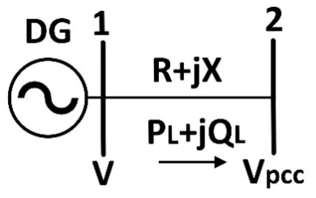
2.1. Power Factor and Power Transfer

In a low-voltage network, the active power flow equation for trading is shown below:

$$P=\frac{V{V}_{PCC}\left(Rcos\delta +Xsin\delta \right)-R{V}_{PCC}^2}{R^2+X^2}$$

(2)

where $V$ and $V_{PCC}$ are the voltages at the output of the DG unit and the PCC, respectively; R and X are the resistance and reactance of the feeders, respectively; and the power angle is marked as δ. The equivalent impedance of the feeder of a low-voltage network is usually dominated by the inductance, considering the influence of the filter and the length, while the resistance can be considered to be a very small value. According to (2), since the maximum output voltage of the DG unit is a certain value limited by the physical equipment, the voltage at the PCC can be reduced by the reactive power requirements from the loads. The smaller the voltage drop ∆V between $V$ and $V_{PCC}$, the more active power is transferred. ∆V can be obtained from (3):

$$\mathsf{\Delta }V=\frac{QX+PR}{V_{PCC}}$$

(3)

As shown in the equation above, for inductive feeders, the ∆V can usually be considered to be related more to reactive power than active power. The less reactive power is compensated, the smaller the voltage drop. At the same time, if the load’s demand for reactive power cannot be effectively met by additional compensation equipment, there will be a significant loss of active power output from the DG according to the theory of energy conservation.

2.2. Economic Value of Reactive Power Demand

In order to increase the capacity of the low-voltage network to transmit active power, i.e., electrical commodities, sufficient reactive resources should be used to keep the voltage levels of the nodes in the low-voltage network within the specified range, so that the network operates efficiently and safely. The adequacy and reasonableness of the reactive resources’ allocation are closely related to the price and quality of the electricity commodity.

The simple power network represented in Figure 1 can be used to illustrate how the value of reactive demand is reflected through opportunity costs in the trading and use of electricity commodities, thus revealing the marginal value of reactive demand.

In Figure 1, nodes 1 and 2 represent the output nodes and grid-connected nodes of the DG units, respectively. $P_{DG}$ and $Q_{DG}$ represent the active output power and reactive output power of the DG, respectively. $P_L$ and $Q_L$ denote the active load power and reactive load power, respectively. $P_l$ and $Q_l$ denote the tidal active and reactive power flowing to the end of the feeder.

Assuming that node 2 has sufficient reactive power resources, the reactive load power of the node just realizes local compensation, which means the power factor of the node is 1 and the reactive power flow from the feeder to the end is 0. At this time, the active power loss of the feeder can be expressed as (4), and the active output power of the DG is the sum of the load and active power loss, as shown in (5):

$$P_{loss}=\frac{P_l^2+Q_l^2}{V_{pcc}^2}\ast R=\frac{R}{V_{pcc}^2}\ast P_L^2$$

(4)

$$P_{DG}=P_L+P_{loss}$$

(5)

In this state, when the active power load is increased by a trace amount on top of the $\mathsf{\Delta }{P}_L$, then the value of the increase in active output power of DG at node 1 is shown in (6). If the marginal price of node 1, where the DG is located, is ${\alpha }_1$, then the marginal price of node 2, where the load is located, is ${\alpha }_2$, as shown in (7):

$$\mathsf{\Delta }{P}_{DG}=\left(1+2\ast P_L\ast \frac{R}{V_{pcc}^2}\right)\mathsf{\Delta }{P}_L$$

(6)

$${\alpha }_2=\frac{{\alpha }_1\ast \mathsf{\Delta }{P}_{DG}}{\mathsf{\Delta }{P}_L}={\alpha }_1\ast \left(1+2\ast P_L\ast \frac{R}{V_{pcc}^2}\right)$$

(7)

It can be seen that the presence of active power losses in the feeder makes a difference in the marginal price between node 1 and node 2, which gives good insight into the analysis of reactive power economics.

If the node 2 reactive power demand needs to be supplied entirely by DG, where the power factor injected by node 2 is not equal to 1, the relationship between the load active power and the load reactive power can always be expressed as $Q_L=k\ast P_L$, where $k$ is a constant calculated from the power factor. If at this point, the DG voltage support is sufficient to keep the node 2 voltage constant and there is also a small increase in the active power of the load $\mathsf{\Delta }{P}_L$, then the output power required to be increased by DG and the marginal price of loads of node 2 can be presented as (8) and (9):

$$\mathsf{\Delta }{P}_{DG}=\mathsf{\Delta }{P}_L+\left(1+k^2\right)\ast \frac{{\left(P_L+\mathsf{\Delta }{P}_L\right)}^2-P_L^2}{V_{pcc}^2}=\mathsf{\Delta }{P}_L+\frac{2\ast \left(1+k^2\right)\ast R\ast P_L}{V_{pcc}^2}\ast \mathsf{\Delta }{P}_L$$

(8)

$${\alpha }_2^{\prime }={\lambda }_1\ast \left(1+\frac{2\ast P_L}{V_{pcc}^2}+\frac{2k^2\ast P_L}{V_{pcc}^2}\right)\ast R$$

(9)

Comparing (9) with (7) shows that, since reactive power flows through the feeder, the active power loss increases while the active marginal price of node 2 increases from ${\alpha }_2$ to ${\alpha }_2^{\prime }$.

Assuming a voltage reduction of $V_{pcc}^{\prime }$, (8) can be rewritten as (10), and the marginal price at node 2 can be expressed as (11):

$$\begin{gathered} \mathsf{\Delta }{P}_{DG}=\mathsf{\Delta }{P}_l+\frac{\left(1+k^2\right)\ast \left[{\left(P_L+\mathsf{\Delta }{P}_L\right)}^2-P_L^2\right]}{V_{pcc}^{\prime }{}^2}\ast R \\ =\mathsf{\Delta }{P}_L+\frac{2\ast \left(1+k^2\right)\ast R\ast P_L}{V_{pcc}^{\prime }{}^2}\ast \mathsf{\Delta }{P}_L \end{gathered}$$

(10)

$${\alpha }_2^{″}={\alpha }_1\ast \left(1+\frac{2\ast P_L}{V_{pcc}^{\prime }{}^2}+\frac{2k^2\ast P_L}{V_{pcc}^{\prime }{}^2}\right)\ast R$$

(11)

As can be seen from (10), in order to meet the reactive power demand of the load, a large amount of reactive power is transferred to the feeder, generating both active power losses, and possibly further increasing active power losses by reducing the voltage at the end nodes, thus giving rise to the relation ${\alpha }_2<{\alpha }_2^{\prime }<{\alpha }_2^{″}$. The marginal value of reactive power demand in the electricity commodity, i.e., the equivalent value of reactive power, can therefore be reflected by the change in the marginal price of active power at the nodes.

The reason why the voltage level at node 2 above cannot be maintained at a constant level is either that the DG is limited in its ability to provide voltage support or that the voltage level is difficult to maintain. If the reactive power demand is completely passive, within a certain voltage level, this will increase the difficulties in the active power output of the power network. Therefore, from the user’s point of view, and in order to safeguard their interests, providing in situ compensation will alleviate this dilemma, which is not only beneficial for the operation of the power network as a whole but also the user. It can be seen that local compensation of reactive power demand is very important for reducing electricity prices, reducing waste of resources, and also ensuring the safety of the operation of the power network. Usually, capacitors, reactors, etc. represent the local compensation of reactive resources, and feeders do not need reactive resources if they operate in the natural power state; below or above the natural power will provide reactive power or absorb reactive power. As can be seen, in the power market environment, the allocation of reactive resources, and by whom, is indeed worth thinking about.

Considering that active transmission causes losses which are usually considered to be a small constant value, the marginal price of active power is consistent at all nodes; the general form of the marginal price at node i is shown in (12):

$${\alpha }_i={\alpha }_{clear}\ast \left(1+\frac{\partial P_{loss}}{\partial P_i}+\frac{\partial P_{loss}}{\partial Q_i}\right)$$

(12)

where ${\alpha }_{clear}$ is the marginal market-clearing price; $\frac{\partial P_{loss}}{\partial P_i}$ is the net loss sensitivity of nodal active injection; and $\frac{\partial P_{loss}}{\partial Q_i}$ is the net loss sensitivity of nodal reactive power injection. (12) shows that the value of reactive power demand is attached to the price of electricity commodities in the electricity market through the incremental cost caused by net loss. It can be seen that the smaller the reactive power demand of an electricity commodity, i.e., the higher the power factor, the lower the price of the electricity commodity; at the same time, the smaller the fluctuation in power factor, the smaller the fluctuation in the price of the electricity commodity.

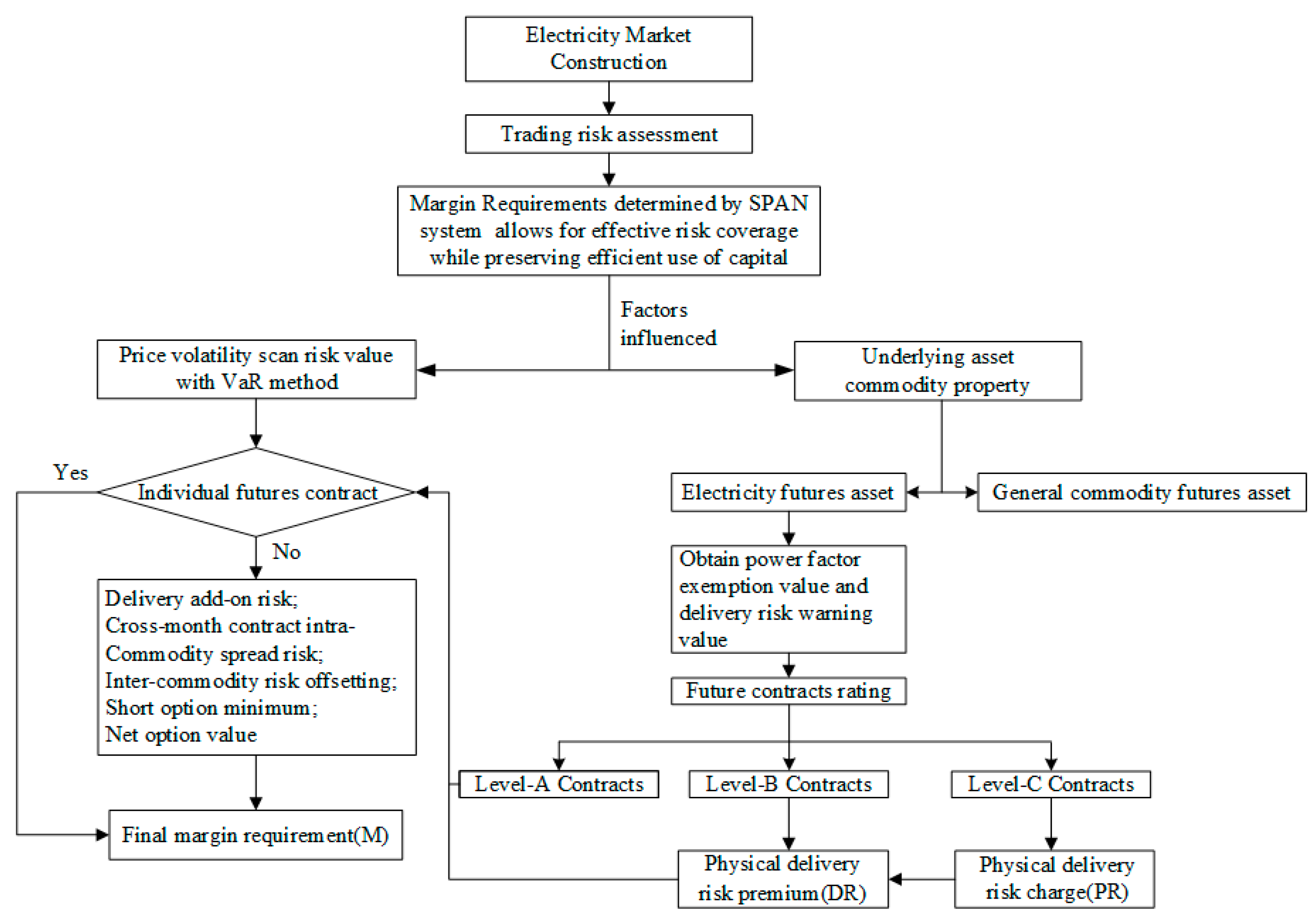
3. SPAN-Based Margin Design for Electricity Futures

3.1. Brief Review of SPAN

The Standard Portfolio Analysis of Risk (SPAN) margining system is a portfolio system used for margining clearing members and customer accounts for futures trading. It evaluates positions and determines collateral requirements based upon estimates of changes in the value of the portfolio consisting of futures and options that would occur under assumed market changes in one day. Margin requirements in the SPAN system are set to cover the largest loss generated by a simulation exercise [25].

SPAN is now a widely used margin system that uses a set of calculation rules that combines all contract positions within a single account as a portfolio and calculates the margin requirement for that portfolio’s exposure to the value at risk (VaR). VaR refers to the expectation that the value of a given portfolio is derived from a certain level of confidence that the maximum loss is likely to occur. At the same time, for portfolios of different commodity groups, SPAN calculates the VaR by taking into account six influencing factors such as price volatility, extreme price changes, cross-month contract spreads for the same commodity, and the offsetting effect of risk between different commodity groups. The actual margin required by the investor is determined by the actual percentage of margin obtained by subtracting the cash flow from the total value at risk from the immediate closing of all options in the position at current market prices.

The core concept of the SPAN system is reflected in its parameterization. For markets in different countries and with different trading policies, SPAN uses a separation of risk control parameters and calculation processes. It is up to the trading markets to set and enter their risk control parameters to reflect the actual trading risks of different markets, in order to calculate margins more accurately. For each portfolio of traded products entered into SPAN, the system calculates and simulates 16 possible scenarios of gain and loss for that portfolio and takes the maximum one as the risk scan value. The system then uses the risk scan value to further calculate indicators such as delivery add-on risk, cross-month contract intra-commodity spread risk, intern-commodity risk offsetting, short option minimum, net option value, etc. to obtain a more accurate margin amount for traders for reference.

3.2. SPAN-Based Margin Calculation

Considering the special characteristics of the underlying assets of electricity power futures, the traditional SPAN system ignores the assessment of some potential risks. In this paper, the non-parametric estimated VaR method will be used to set the risk scan values and incorporate a delivery risk assessment method applicable to the risk assessment of the underlying asset of new energy assets. As electricity options are currently outside our scope, this paper only improves the SPAN system for risk assessment of individual contracts in the futures trading process. In this paper, the margin is expressed in terms of the asset portfolio risk value, with the addition of the electricity quality delivery risk value, as shown in Equation (13):

$$M=VaR\left(1+RP\right)+DR$$

(13)

where VaR is the value at risk of the electricity contract and RP and DR are the physical delivery risk premium and the physical delivery risk charge, respectively, for different contract ratings. The process of the whole margin calculation should follow the instructions as illustrated in Figure 2.

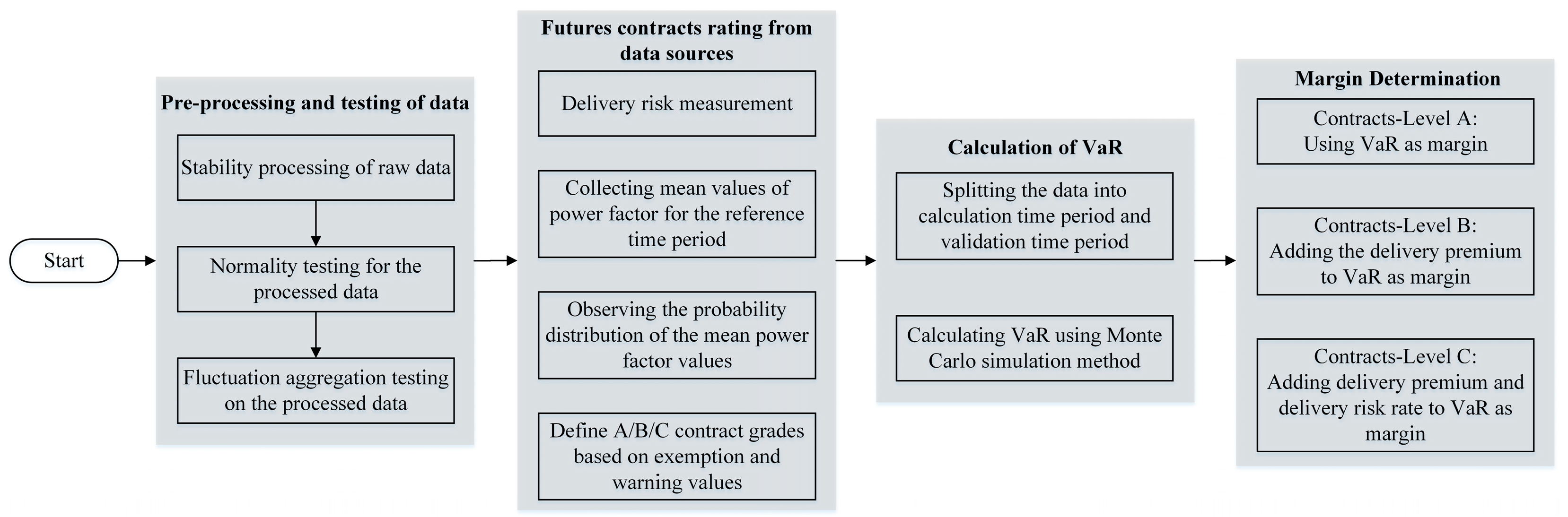
3.2.1. Value at Risk (VaR) Calculation

The SPAN system evaluates the scan risk parameters requiring a price scan interval, which is represented by the VaR in this paper. VaR is the potential maximum loss that could be caused for a portfolio if the value of the portfolio changes for a given holding period and at a given confidence level, as shown in Equation (14):

$$Prob\left(\Delta p<-VaR\right)=1-\alpha$$

(14)

where Δp represents the loss amount of the portfolio over the holding period and VaR is the value at risk at the confidence level α.

Among the VaR methods, the Monte Carlo simulation is able to be set up flexibly for the actual distribution that price fluctuations follow, and can have high predictive accuracy, especially for scenarios where the fluctuations are large and the distribution shows a thick tail phenomenon. In capital markets, geometric Brownian motion is the most widely used stochastic model to describe the prices of financial assets; it assumes that, over a relatively short period of time, asset value changes are independent of the time series, as in Equation (15) shown below:

$$\mathsf{\Delta }S=\mu S\mathsf{\Delta }t+\sigma S\epsilon \sqrt{\mathsf{\Delta }t}$$

(15)

where $\mathsf{\Delta }S$ concerns assets over the period $\mathsf{\Delta }t$, the change in $\mu$ is the expected value of the yield, $\sigma$ is the volatility of the return, and $\epsilon$ is the set of random numbers obeying the standard normal distribution.

If the n randomly generated random numbers are currently defined as ${\epsilon }_i\left(i=1,2,3\dots n\right)$, and the current observation time period is t, and the future time point at which the simulation will be performed is T (T > t), the time period will be divided into n simulated asset prices calculated according to Equation (15) as $S_1,S_2,S_3\dots S_n$; at this time, $\mathsf{\Delta }t=\frac{\mathrm{T}-\mathrm{t}}{n}$, and then using the current market price of the asset as the initial price, this can be used to find the n simulated asset prices:

$$\left\{\begin{array}{c}{S}_1=S_0+\mu S_0\mathsf{\Delta }t+\sigma S_0\epsilon \sqrt{\mathsf{\Delta }t}\\ S_2=S_1+\mu S_1\mathsf{\Delta }t+\sigma S_1\epsilon \sqrt{\mathsf{\Delta }t}\\ \dots \\ S_n=S_{n-1}+\mu S_{n-1}\mathsf{\Delta }t+\sigma S_{n-1}\epsilon \sqrt{\mathsf{\Delta }t}\end{array}\right.$$

(16)

At this point, $S_n$ is one possible rate of return at time t. The process is simulated iteratively to give K∙values of $S_n$; the sequence is ranked in descending order and, based on the ranking result, takes α% of the possible closing index return value of the ranked K(1 − α). The VaR value under the confidence level (1 − α) is calculated.

3.2.2. Physical Delivery Risk Rates

Given the special problems of electricity assets due to the uncertainty of new energy sources, when a futures contract is close to delivery, a delivery premium will be demanded underlying commodities whose power factor cannot reach the exempted value $P{F}_{ex}$. The delivery premium rate is $RP$. In the case that the electricity supplier is unable to close a futures contract at the delivery date due to a low power factor and poor quality of electricity, to protect traders and to act as a warning to suppliers, such a type of non-deliverable electricity futures contract is subject to delivery risk charge $DR$. The delivery premium and the delivery risk charge rate are determined by the power factor exemption value $P{F}_{ex}$ and the average value of the delivery risk warning value $P{F}_{loss}.$ The Power Factor $PF$ is measured as the average value over a certain period of time, which is usually taken as a short period. $P{F}_{ex}$ and $P{F}_{loss}$ are generally determined based on the probability of occurrence of historical data on electricity provided by the supplier, and the delivery risk charge rate $r$ is determined by the exchange and is calculated as follows:

• Step 1: The exchange determines the power factor exemption value based on the requirements of the futures contract $P{F}_{ex}$ and the average value of the delivery risk warning value $P{F}_{loss}$.
• Step 2: Select the actual power factor sampling time period T and acquire m data points in the time period according to the unit time t: $S_1,S_2,S_3,\dots S_m$.
• Step 3: Count the frequency distribution of all data points and observe the distribution.
• Step 4: Select the percentage of the distribution where the power factor is less than the exemption value required: $Pro{b}_{ex}=prob(S_i<P{F}_{ex})$.
• Step 5: Select the percentage of the distribution where the power factor is less than the delivery risk warning value required: $Pro{b}_{loss}=prob(S_i<P{F}_{loss})$.
• Step 6: Calculate the delivery premium and delivery risk rate.

In summary, the physical delivery risk can be calculated using Equation (17):

$$\left\{\begin{array}{c}PR=1-Pro{b}_{ex}\\ DR=\left(1-Pro{b}_{loss}\right)\ast r\end{array}\right.$$

(17)

In Equation (17), PR refers to physical delivery risk premium and DR refers to delivery risk charge. $Pro{b}_{ex}$ is the probability that the underlying asset is capable of physical delivery at contract maturity but cannot be delivered by the contract units. $Pro{b}_{loss}$ is the probability that there will be a significant loss of power quality at maturity, resulting in the inability to take physical delivery; $r$ is the delivery risk charge rate, which may be determined at the discretion of the exchange. When the power factor is greater than $P{F}_{ex}$, the margin on the futures contract is the value at risk; when the power factor is between $P{F}_{loss}$ and $P{F}_{ex}$, the physical delivery risk premium is added. When the power factor is less than the $P{F}_{loss}$, a physical delivery risk charge is added to the margin, taking into account the disruption to the overall trading market caused by power quality.

3.2.3. SPAN-Based Margin Calculation Model

The electricity quality assessed by the power factor (PF) represents the delivery quality of the underlying asset, and this paper classifies electricity futures contracts into three levels, A, B, and C. Level-A contracts have a delivery power quality that exceeds the power factor exemption value and can be delivered following the contract unit. The power of Level-B contracts is less than the power factor exemption value $P{F}_{ex}$ but greater than the delivery risk warning value $P{F}_{loss}$. Although the contract has the risk of a small loss of power at the time of delivery, the physical delivery can still be ensured, and the probability of loss can be captured; the quality of electricity for the delivery of Level-C contracts is less than the delivery risk warning value $P{F}_{loss}$. It might be risky that physical delivery will not be achieved. The margin calculation for these three types of electricity futures contracts is shown as Equation (18):

$$\left\{\begin{array}{c}M=VaR, PF\ge P{F}_{ex}\\ M=VaR\left[1+\left(1-Pro{b}_{ex}\right)\right], P{F}_{ex}>PF\ge P{F}_{loss}\\ M=VaR\left[1+\left(1-Pro{b}_{ex}\right)\right]+\left(1-Pro{b}_{loss}\right)\ast r, PF<P{F}_{loss}\end{array}\right.$$

(18)

The values obtained according to (18) can be entered into the SPAN system as price scan intervals for further evaluation of the scan risk parameters.

4. Empirical Study

The empirical study process followed the steps shown in Figure 3.

4.1. Data

The data was chosen from daily future price data for PJM Western Hub real-time peak electricity from NYMEX. The time period spans from 11 March 2017 to 11 March 2022. The contract is currently in cash settlement and meets the requirements of a Level-A contract as defined in the previous section. In order to make the data series stable and prepared for VaR calculation, the daily log returns for the above time period are selected as a sample in this paper by using Equation (19):

$$r_t=\ln \left(P_t\right)-\ln \left(P_{t-1}\right)$$

(19)

where $r_t$ refers to the daily log return, $P_t$ refers to the futures contract price at time t, and $P_{t-1}$ refers to the futures contract price one day before time t.

Given a confidence level of 95%, the VaR for the next trading day is calculated using the Monte Carlo method. The VaR indicating the maximum loss value for that day is the price scan interval applied by the SPAN system for that trading day.

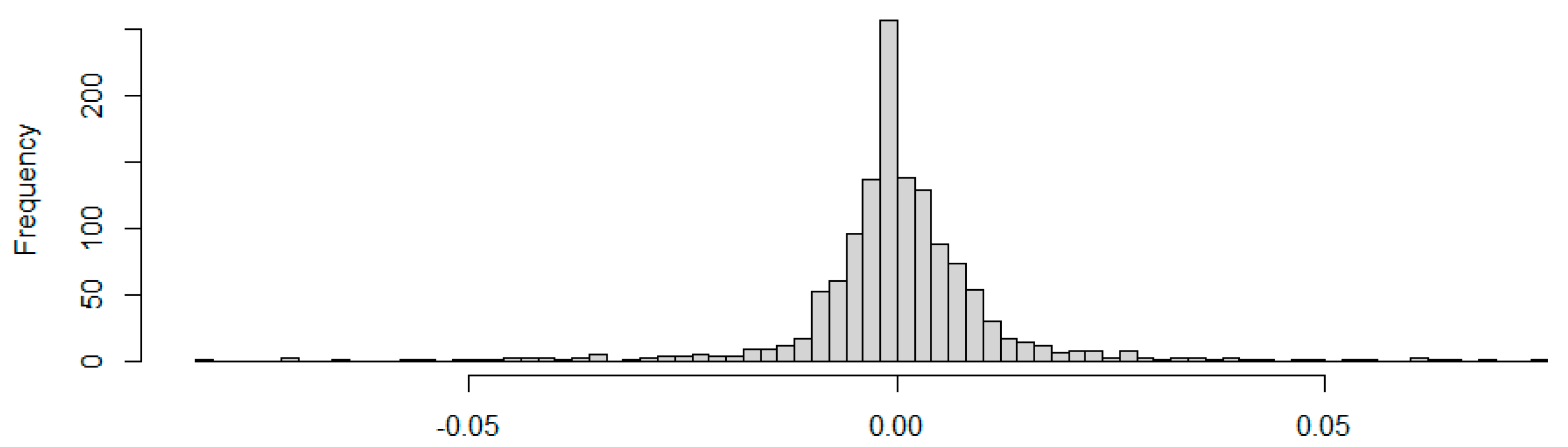
4.2. Summary Statistics

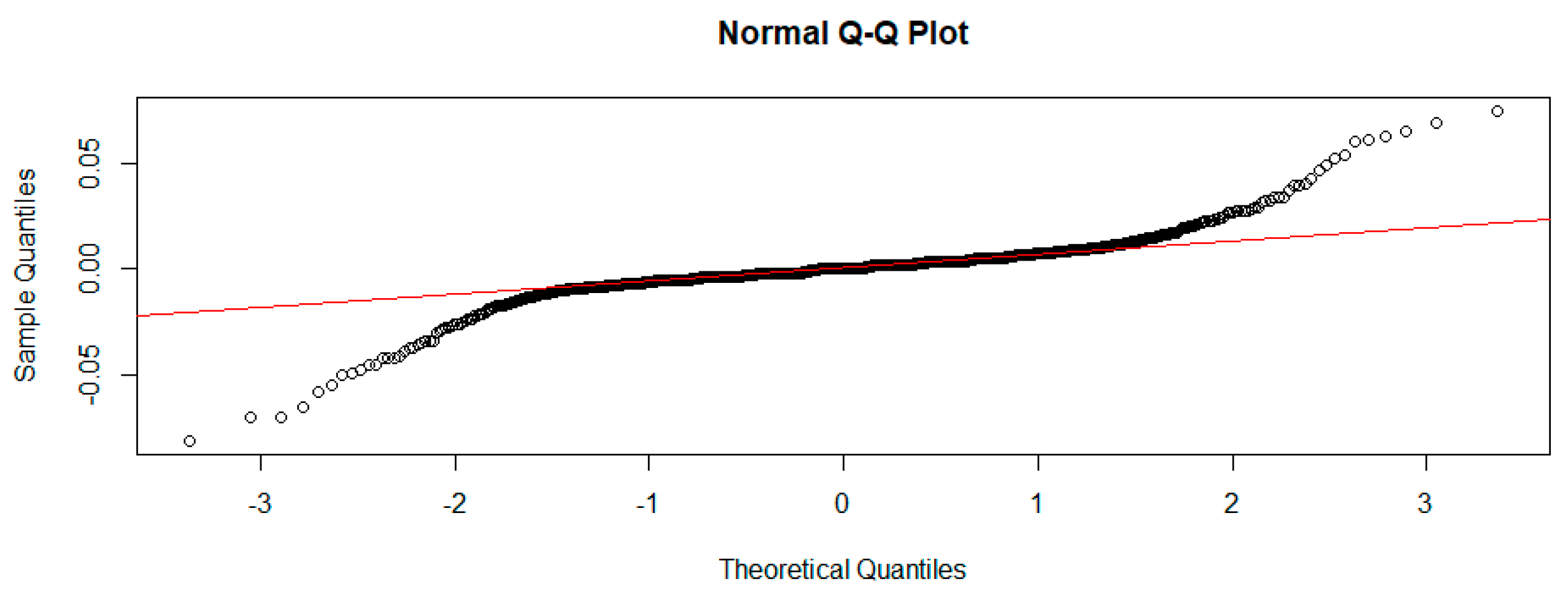
4.2.1. Normality Test (Quantile–Quantile Plot)

The quantile–quantile plot (Q–Q plot) is a more intuitive and effective way to test the normality of the data. If the Q–Q plot of the data shows a linear trend, this means that the selected sample satisfies a normal distribution; if the graph shows non-linear characteristics, then the sample is not normally distributed. The quantile–quantile plot for the selected sample in this paper is shown in Figure 4.

As can be seen from Figure 4, the quantile–quantile plot of the selected data is non-linear, with large deviations in the tails, so the sample is not normally distributed.

4.2.2. Normality Test (Jarque-Bera Test)

After the initial determination of sample normality, the Jarque-Bera statistic was constructed and tested according to the value of the statistic, where the expression of the statistic is as follows:

$$JB=\frac{N}{6}\left[S^2+\frac{1}{4}{\left(K-3\right)}^2\right]$$

(20)

where N is the sample size and K and S are the kurtosis and skewness of the sample data, respectively. For a thick-tailed distribution, the kurtosis should be greater than 3. Therefore, it is necessary to first perform a descriptive analysis of the data to find the value of its descriptive statistics. The Jarque-Bera test for the data used in this paper is shown in

Table 1. Jarque-Bera statistics for data selected.

Mean	Median	Maximum	Minimum	Stdev	Skewness	Kurtosis	Jarque-Bera	p-Value
0.0004	0.000	0.0750	−0.0813	0.0119	−0.1253	11.1845	6821.523	0.000

. The distribution of selected data is shown as a histogram in Figure 5.

From Table 1 and Figure 5, the J-B statistic for the daily return on the PJM futures contract is 6821, with a skewness of −0.1253 and kurtosis of 11.1845, showing the characteristics of a sharp peak with a thick tail. Therefore, the sample does not follow a normal distribution.

4.2.3. Volatility Clustering Test

The easiest and most intuitive way to test for volatility clustering is to generate the time series plot of returns for the data and observe its volatility over each period. The time series volatility clustering of returns for the PJM futures in the selected period is shown in Figure 6.

From Figure 6, it can be visualized that the daily returns on the sample data are less volatile over a certain period of time, while over a very short period, the returns on this sample are more volatile, from which it can be obtained that there is a clear volatility clustering in the PJM electricity futures contract market.

4.3. Calculation Results

The VaR for the 12 March 2022 PJM futures contract can be calculated by the method described above as follows:

Step 1: Calculate the yield using the closing price of the PJM peak hour contract for the 1304 trading days from 11 March 2017 to 11 May 2022. Divide the one-day holding period into 16 equal parts and calculate the mean and standard deviation of the contract’s yield for each time period $\frac{\mu }{16}$ and standard deviation $\frac{\sigma }{16}$. The mean and standard deviation of the contract returns for each time period are calculated.

Step 2: Generate 16 random numbers following the standard normal distribution ${\epsilon }_1,{\epsilon }_2,{\epsilon }_3\dots {\epsilon }_{16}$ and substitute the initial price $S_0$ with the 16 random numbers in Equation (15) to simulate a trajectory of the contract price.

Step 3: Put $S_0$ (the closing price of the futures contract on 11 March 2022), $\frac{\mu }{16}$, $\frac{\sigma }{16}$, and ${\epsilon }_i$ into Equation (16) to obtain the simulated futures contract price $S_T$. This is a possible closing price for the futures contract on 12 March 2022.

Step 4: Repeat times steps 2 and 3 6000 times to predict a range of possible closing prices for the futures contract on 12 March 2022: $S_T^1,S_T^2,S_T^3\dots S_T^{6000}$.

Step 5: Arrange this closing price series obtained in step 4 in descending order; the 300th figure is the quantile of this series at the 95% confidence level, that is, the forecast price of futures for that day at the 95% confidence level. Then, the VaR value is $S_0-S_T^{min5\%}$.

The simulated value at risk for the PJM futures contract on 12 March 2022 was calculated to be $89.58 per contract, which is the price scan interval for the contract in the SPAN system and is the amount of margin that should be charged for the contract on 12 March 2022 as given in the SPAN system. The margin required on 12 March 2022 was calculated to be $182.5 per contract using the traditional margin calculation with a fixed margin ratio, which is much higher than the margin required under the SPAN system.

The method above was repeated 42 times to attain the simulated amount of margin that should be charged on the SPAN system for the 42 trading days from 12 March 2022 to 12 May 2022 for the PJM futures contract.

Through the above calculation process, the margin amount for the Level-A contract can be obtained. This can be compared with the amount of margin required for one electricity futures contract under the proposed margin system on one day and the actual loss amount for that contract on that day, the results of which are shown in Figure 7.

Figure 7 shows a comparison of the amount of margin requirement calculated by the proposed method, actual risk, and the amount of margin requirement obtained by the fixed ratio of the electricity future contract value. The actual risk is the absolute value of daily log returns on these prices by following the Equation (19) from 12 March 2022 to 12 May 2022. The fixed ratio of margin requirement was set as 5% of the futures contract value, referenced from the initial margin requirement ratio from leading futures exchanges in North America. It can be seen from Figure 7 that the margin calculated by the proposed method is always higher than the actual risk, which means such a margin requirement can cover all the risk of possible price fluctuations. Furthermore, the amount of margin is much lower than the current margin, which is determined by a fixed ratio of the value of the futures contract. This confirms that the margin requirement calculation proposed in this paper reduces trading costs (investors trade the same position with a lower margin payment) and covers the market risk.

5. Conclusions

The implementation of the green power futures market will effectively improve the penetration of renewable energy and reduce the carbon emissions of the power system. However, the risks of green power are more diverse, among which the risks based on power factors are more prominent when compared with traditional futures. An electricity power futures market margin calculation method that considers the impact of the power factor is proposed in this paper, to evaluate the power market risk based on green power futures. First, the impact of power factor changes on energy transmission and physical delivery of green power futures is analyzed; second, a dynamic margin calculation method based on the SPAN system is proposed. Next, a futures contract rating method based on historical power factor data is proposed, and a margin design method considering power factor risk is proposed under the rating. In order to verify the effectiveness of the dynamic margin calculation method, an empirical demonstration is conducted in this paper. According to the empirical results, the dynamic margin level can cover the risk value of futures contracts, and is significantly lower 50% more than the actual margin amount charged under the traditional strategic margin model, which proves that the proposed calculation method can effectively meet the safety, liquidity, and profitability requirements of the electricity power futures market. It must be acknowledged that such a margin calculation method was verified by using a single electricity future contract. Thus, for more complex trading situations (such as the portfolios of futures contracts with both buy and sell orders), the combination of futures and options, the complex electricity market derivatives with financial attribute trading strategies for hedging rather than physical delivery, additional risk assessment procedures (especially for the hedging strategies), and the pricing of electricity options represent other promising areas of study which could be addressed in future research.

References

1. Lin, J.; Kahrl, F.; Yuan, J.; Liu, X.; Zhang, W. Challenges and strategies for electricity market transition in China. Energy Policy 2019, 133, 110899. [Google Scholar] [CrossRef]
2. Spodniak, P.; Bertsch, V. Is flexible and dispatchable generation capacity rewarded in electricity futures markets? A multina-tional impact analysis. Energy 2020, 196, 117050. [Google Scholar] [CrossRef]
3. Zhang, Y.; Farnoosh, A. Analyzing the dynamic impact of electricity futures on revenue and risk of renewable energy in China. Energy Policy 2019, 132, 678–690. [Google Scholar] [CrossRef]
4. Deng, W.; Dai, N.; Lao, K.-W.; Guerrero, J.M. A Virtual-Impedance Droop Control for Accurate Active Power Control and Reactive Power Sharing Using Capacitive-Coupling Inverters. IEEE Trans. Ind. Appl. 2020, 56, 6722–6733. [Google Scholar] [CrossRef]
5. Deng, W.; Liu, Z.; Qin, H.; Chen, M.; Zhang, Y. Study of a virtual-impedance of the capacitor-series inverter for wider ac-curate power control range. Energy Rep. 2022, 8, 27–36. [Google Scholar] [CrossRef]
6. Tang, Y.; Zhuang, Z.; Li, X. Revision Suggestion on the Policy of Tariff Regulation by Power Factor. Power Capacit. React. Power Compens. 2009, 30, 15–20. [Google Scholar]
7. Lien, D.; Yang, L. Availability and settlement of individual stock futures and options expiration-day effects: Evidence from high-frequency data. Q. Rev. Econ. Finance 2005, 45, 730–747. [Google Scholar] [CrossRef]
8. Adil, F.; Siddiqui, D.-A. Exploring the Effect of Physical Delivery Verses Cash Settled Futures Contracts with the Prospective of Obligatory Delivery in Islamic Contract of Sales. Int. J. Soc. Adm. Sci. 2019, 4, 155–177. [Google Scholar] [CrossRef] [Green Version]
9. He, Y.; Su, F.; Xia, Y. PJM Electric Future Trading Experience and Its Enlightment to Electric Future Construction in China. Guangdong Electr. Power 2021, 34, 37–42. [Google Scholar]
10. Huisman, R.; Kilic, M. Electricity Futures Prices: Indirect Storability, Expectations, and Risk Premiums. Energy Econ. 2012, 34, 892–898. [Google Scholar] [CrossRef]
11. Al Boucherbi, M.; Askari, Q. Modern financial investment tools, future contracts as a model. Eurasian J. Hist. Geogr. Econ. 2022, 9, 22–32. [Google Scholar]
12. Klimontowicz, M.; Losa-Jonczyk, A.; Zacny, B. Banks’ Energy Behavior: Impacts of the Disparity in the Quality and Quantity of the Disclosures. Energies 2021, 14, 7325. [Google Scholar] [CrossRef]
13. Pressmair, G.; Amann, C.; Leutgöb, K. Business Models for Demand Response: Exploring the Economic Limits for Small- and Medium-Sized Prosumers. Energies 2021, 14, 7085. [Google Scholar] [CrossRef]
14. Fishe, R.P.H.; Goldberg, L.G.; Gosnell, T.F.; Sinha, S. Margin requirements in futures markets: Their relationship to price volatility. J. Futur. Mark. 1990, 10, 541–554. [Google Scholar] [CrossRef]
15. Wang, J.; Ge, Y.; Tang, K.; Deng, Y. Can Adjustments of Futures Trading Rules Reduce Investor’s Leverage? J. Man-Agement Sci. China 2019, 24, 99–110. [Google Scholar]
16. Sun, Q.; Liang, Z.; Wang, X.; Zheng, W. Research on Dynamic Calculation Method of Margin in Electricity Market-Design of calculation method based on electricity price characteristics and SPAN system. Price Theory Pract. 2021, 7, 145–150. [Google Scholar]
17. Si, J.; Huang, R.; Gong, P. Nonparametric VaR Method′s Application in Standard Portfolio Analysis of Risk. Journal of Wuhan University of Technology. Transp. Sci. Eng. 2007, 31, 664–667. [Google Scholar]
18. Kupiec, P.H.; White, P. Regulatory competition and the efficiency of alternative derivative product margining systems. J. Futures Mark. 1997, 16, 943–969. [Google Scholar] [CrossRef] [Green Version]
19. Eldor, R.; Hauser, S.; Yaari, U. Safer Margins for Option Trading: How Accuracy Promotes Efficiency. Multinatl. Finance J. 2011, 15, 217–234. [Google Scholar] [CrossRef]
20. Zhao, Z.; Cheng, R.; Yan, B.; Zhang, J.; Zhang, Z.; Zhang, M.; Lai, L.L. A dynamic particles MPPT method for photovoltaic systems under partial shading conditions. Energy Convers. Manag. 2020, 220, 113070. [Google Scholar] [CrossRef]
21. Alexander, C.; Kaeck, A.; Sumawong, A. A parsimonious parametric model for generating margin requirements for futures. Eur. J. Oper. Res. 2018, 273, 31–43. [Google Scholar] [CrossRef]
22. Westgaard, S.; Frydenberg, S.; Sveinsson, J.A.; Aalokken, M. Performance of value-at-risk averaging in the Nordic power futures market. J. Energy Mark. 2021, 13, 25–55. [Google Scholar] [CrossRef]
23. Guo, Z. Stochastic multifactor models in risk management of energy futures. J. Future Mark. 2020, 40, 1918–1934. [Google Scholar] [CrossRef]
24. Pena, J.I.; Rodriguez, R.; Mayoral, S. Tail risk of electricity futures. arXiv 2020, arXiv:2202.01732. [Google Scholar]
25. Cotter, J.; Dowd, K. Extreme spectral risk measures: An application to futures clearinghouse margin requirements. J. Bank. Finance 2006, 30, 3469–3485. [Google Scholar] [CrossRef] [Green Version]
Figure 1. A simplified topology of low-voltage power network.
Energies 15 05138 g001
Figure 2. An overview of SPAN-based margin calculation.
Energies 15 05138 g002
Figure 3. Step flow of empirical study.
Energies 15 05138 g003
Figure 4. Quantile–quantile plot of selected data.
Energies 15 05138 g004
Figure 5. PJM Western Hub Peak data distribution.
Energies 15 05138 g005
Figure 6. PJM Western Hub Peak log return series plot.
Energies 15 05138 g006
Figure 7. Comparison of the absolute values of margin and actual loss amounts.
Energies 15 05138 g007