1. Introduction
Photovoltaic (PV) systems represent one of the fastest growing renewable energy sectors [
1]. However, industry analysis shows that there has been a persistent gap between expected and observed energy generation at PV sites, which impacts the overall revenue generated at a PV site [
2]. These inconsistencies arise from a combination of deviations, from overestimations in baseline values [
3] to failures observed within the field. The latter can arise from diverse causal mechanisms within PV, including delamination within modules [
4], communication system problems within inverters [
5], and exposure to extreme weather events [
6].
Given the notable impact that reduced production can have on overall PV site revenue [
2], significant attention has been given to failure detection and diagnosis methods to improve the reliability of these systems and reduce system downtime. Diverse types of data have been used to characterize failures, including current–voltage traces [
7], electroluminescence/infrared imagery data [
8], and maximum power points [
9]. Researchers have also evaluated operations and maintenance (O&M) tickets to understand seasonal patterns in failure frequencies to inform operators of common failure modes and support planning efforts [
5].
Machine learning (ML) approaches, such as neural networks (NNs), have emerged as popular techniques for failure characterizations. For instance, artificial NNs have been trained with solar irradiance and PV temperature measurements to classify large deviations observed in real time between measured and predicted power values [
10]. Others have used convolutional NNs to predict the daily electrical power curve of a PV panel using the power curves of neighboring panels to support the detection of panel malfunctions [
11]. Alternatively, distance metrics have been used as part of supervised cluster-based analyses to determine failures relative to deviations from normal clusters of events observed from the time series of non-degraded PV sensor data [
12,
13,
14].
NN methods have demonstrated significant potential for failure analyses. However, the limited nature of labeled datasets used to train and validate these algorithms makes it is unclear whether the trained models can generalize well across exogenic variables such as site-specific characteristics, micro-climates, and seasonality trends [
15]. Furthermore, interpretability issues surrounding ML architectures render the estimation and uncertainty quantification of explainable parameters that regulate PV systems as difficult [
16]. Finally, cluster-based approaches cannot quantify valuable information (e.g., the average time to failure) necessary for both accurate maintenance prediction and risk analyses of a variety of systems.
In contrast, unsupervised statistical methods for failure analyses are able to work with smaller unlabeled data and use a probabilistic approach for identifying patterns within datasets. For example, failure patterns have been characterized using curve fitting methods to generate parameters from the Weibull distribution (parametric approach) and to generate survival functions (non-parameteric approach) [
17]. Markov processes and stochastic processes with the special property that their future and past realizations (or
states) are independent given their present state and have also been used to characterize the mean times to failure in PV systems [
18]. Although survival rates and times to failure are quantifiable and well-characterized, these approaches focus more on characterization vs. detection.
In this paper, we extend these statistical implementations by introducing the photovoltaic-hidden Markov model (PV-HMM) to support failure detection needs. The popularity of HMMs arises from their ability to relate sequences of observations (or
emissions) with an underlying Markov process, whose unobserved (i.e., hidden) states form the target of inference. HMMs are able to work with discrete time series (e.g., hourly measurements), which makes this method particularly well suited for characterizing and predicting failures in solar PV. Markov Chains (i.e., Markov processes in discrete time) with probabilistic functions in the form of HMMs have been extensively used in many scientific disciplines, including speech recognition [
19], bioinformatics [
20], and epidemiology [
21]. HMM implementations have also entered energy domains, with researchers using this method to predict energy consumption in buildings [
22], evaluate battery usage patterns [
23], and even explore fault diagnosis with simulated data in wind energy systems [
24]. In this analysis, we extend these implementations to characterize field failures at PV sites.
Specifically, we train site-specific PV-HMMs to distinguish and extrapolate failure states from performance signals in an unsupervised manner with relatively little data. The main benefit of this novel approach are that HMMs do not require labels to train the models and perform robustly even with coarse data [
22]. Comparison analyses with threshold levels (TLs) and O&M tickets are used to validate the model outputs. In addition to advancing our understanding of transitions between normal and faulted states, this method can also be used to support predictive maintenance efforts within PV and other energy industries working with similar datasets. The remainder of this paper describes the HMM model and datasets in greater detail (
Section 2), presents the results of the trained PV-HMM models (
Section 3), and concludes with implications of the analysis and future work opportunities (
Section 4).
2. Materials and Methods
This analysis was supported by Sandia National Laboratories’ PV reliability, operations, and maintenance (PVROM) database, which contains production, environmental, and O&M ticket data for multiple sites across the United States [
6]. More information about the database contents, as well as the data processing and training of PV-HMMs, is described in the following sub-sections.
2.1. Data and Pre-Processing
The PVROM database contains co-located production and maintenance data for 186 sites across the United States [
6]. Production datasets from each site generally capture continuous temporal measurements of observed energy production as well as onsite environmental measurements (e.g., irradiance and temperature) that are measured at regular intervals (e.g., every hour). Site O&M tickets, on the other hand, are discrete data points that are generated whenever an issue is observed that requires tracking or maintenance at a site. O&M tickets generally capture information about the date the issue was first observed, a general description of the issue, and details about how/when the issue was resolved.
Site-level data from PVROM require cleaning and filtering to ensure that the collected data meet quality standards. Following previous analyses [
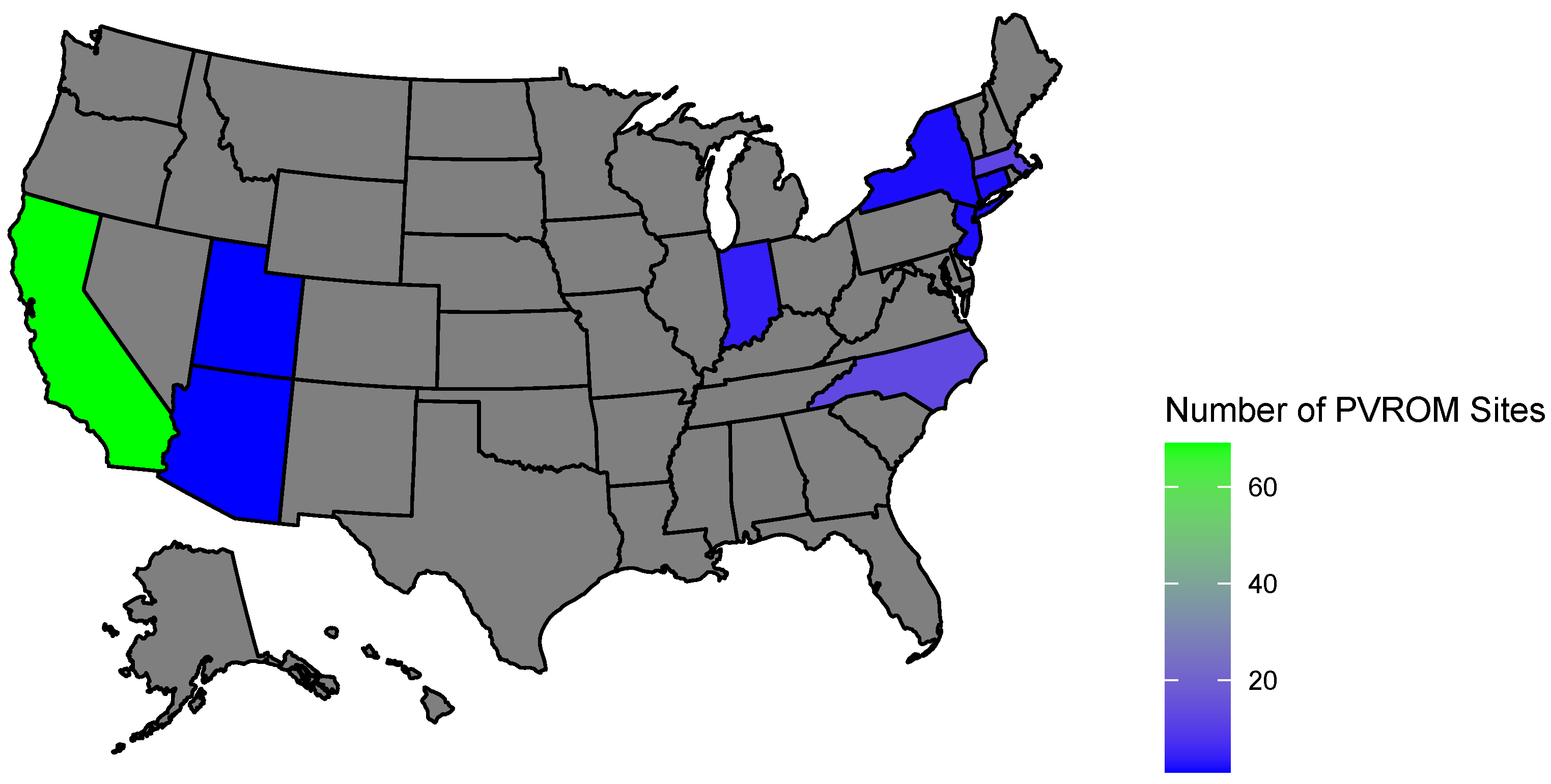
3], various filters were used to remove non-negative energy values and verify that the energy capacity constraints of each site were met. In addition, time periods with irradiance values greater than 400 Watts per square meter irradiance were retained to capture active production hours. Only sites that contained at least 25 data points post data quality checks were considered for further analyses. The final dataset used for PV-HMM analyses consisted of approximately 200,000 hourly data points across 104 sites in nine states across the United States (
Figure 1). Generally, the number of data points per site ranged from 170 to 3300.
After data cleaning, data processing steps, involving the normalization of production data and tagging periods with active O&M tickets, were conducted. Specifically, the observed energy production (E) was normalized at each site with the associated expected energy values provided by the industry site operator (). The resulting metric is known as the performance index (), which is the primary variable of interest for PV-HMM analyses. Normalizing the energy by a baseline removes the variance caused by normal operation, such as periodic behavior resulting from sunrises and sunsets, and renders a signal which is mainly centered around one. Large perturbations from one, however, may imply a system anomaly and indicate a faulted system. Finally, to support model evaluation activities, PI values were tagged with a flag to indicate whether there was an active O&M ticket for a given hour at a site.
2.2. Photovoltaic Hidden Markov Model (PV-HMM)
Here, we describe the hidden Markov model and its application to PV in greater detail. Specifically, the PV-HMM relates the univariate signal underlying system performance with what is observed of performance indices. A PV-HMM is trained per site using hourly PI data.
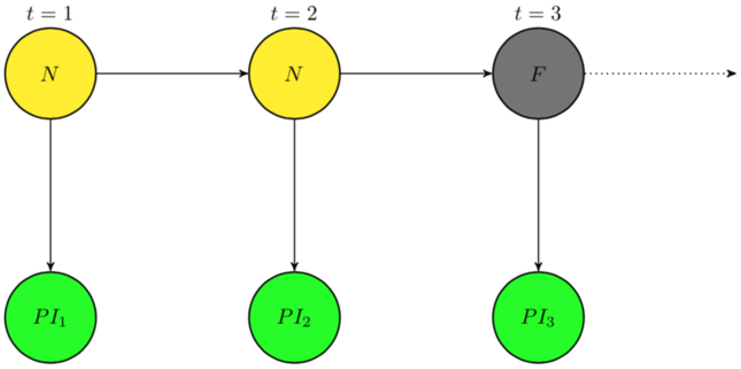
The PV-HMM is intended to learn the states of a 2-state discrete time Markov chain denoted as
over time
, where
n denotes the hours that PI is analyzed. We assume that its states are binned according to normal (N) and faulted (F) signals, enabling
. This chain is characterized first by its initial probability of being in state N,
(or equivalently
). Second, due to the
Markov property or the conditional independence of past and future states on the present state, i.e.,
, its transition matrix is
, meaning that the one-step transition probabilities
between all states are also required in its characterization. Here,
whose rows sum to one, providing an alternative representation of the state space diagram for
, as shown in
Figure 2. The measured performance indices
at each discrete time point
can be related to the underlying states
, as depicted in
Figure 3, via fitted emission densities of the form:
Here,
f denotes a general probability density function depending on
and other parameters
and is commonly taken to be the Gaussian distribution for continuous responses or the multinomial distribution for categorical (discrete) responses. However, faulted states could occur at both high and low PI values so a bi-modal distribution is possible that would violate Gaussian assumptions. To deal with this, we utilize
a 2-component Gaussian mixture model (GMM) that is able to more effectively capture nuances in the performance indices. Here,
, including the mixing proportion of the densities
, and unknown mean (
) and standard deviation (
) parameters for each mixture that depend on the state of the underlying Markov chain. Estimating such parameters from the HMM enables predictions to be made between future performance indices and the state of the PV system. This can be achieved by using an iterative quasi-maximization approach called the Baum–Welch algorithm, a type of expectation–maximization (EM) algorithm [
25]. At each iteration, this algorithm first performs an expectation (E) step by evaluating the derived expected log-likelihood function at current parameter estimates. Second, a maximization step (M) is pursued to iteratively update parameter estimates until their change becomes negligible and a quasi-maximum is found. Using these parameters, the Viterbi algorithm, a dynamic programming regime, can then be applied to obtain the most likely sequence of labels (N,F) for the hidden states of the PV system. A more thorough introduction to the Viterbi algorithm and its formulation for general inference in HMMs can be found at [
26,
27].
2.3. Model Evaluation
The performance of failure detection algorithms is commonly evaluated by way of comparison with other physics-based or NN algorithms [
28]. Such approaches, however, only work in simulated settings when the system state is truly known [
24,
29]. In contrast, one of the biggest challenges for field-based PV failure analyses is the lack of ground truth available for field observations. Since the true system state is not well known for our data, we use two approaches to evaluate PV-HMM generated outputs: TLs and O&M tickets. Thresholds are a common method used in PV failure detection implementations due to their relative simplicity of use [
30]. In this analysis, we generate TLs using a percentile approach, wherein data points were compared to different percentiles associated with each site data. At each percentile TL, data that were greater than the associated threshold were flagged as indicating the associated system state. A comparison of these patterns with associated transition probabilities of the PV-HMM enables us to evaluate the general range of TLs, whereby similar probabilities are observed.
As noted above, the TLs provide a basis of comparison but do not necessarily reflect field confirmation. Therefore, the threshold comparisons were augmented by comparing PV-HMMs with O&M tickets, which can capture some observed failures. Previous analyses, however, have indicated that O&M tickets do not capture all possible failures observed at a site [
31]. Therefore, evaluation assessments focused on precision analysis to quantify the percentage of O&M tickets that corresponded to a faulted state, as identified by PV-HMMs. A precision metric can be reliable under the assumption that the notated tickets are accurate, without necessarily assuming that the labeling process was comprehensive. The precision metrics are supplemented by site-level visualizations to generate qualitative insights into PV-HMM performance.
3. Results
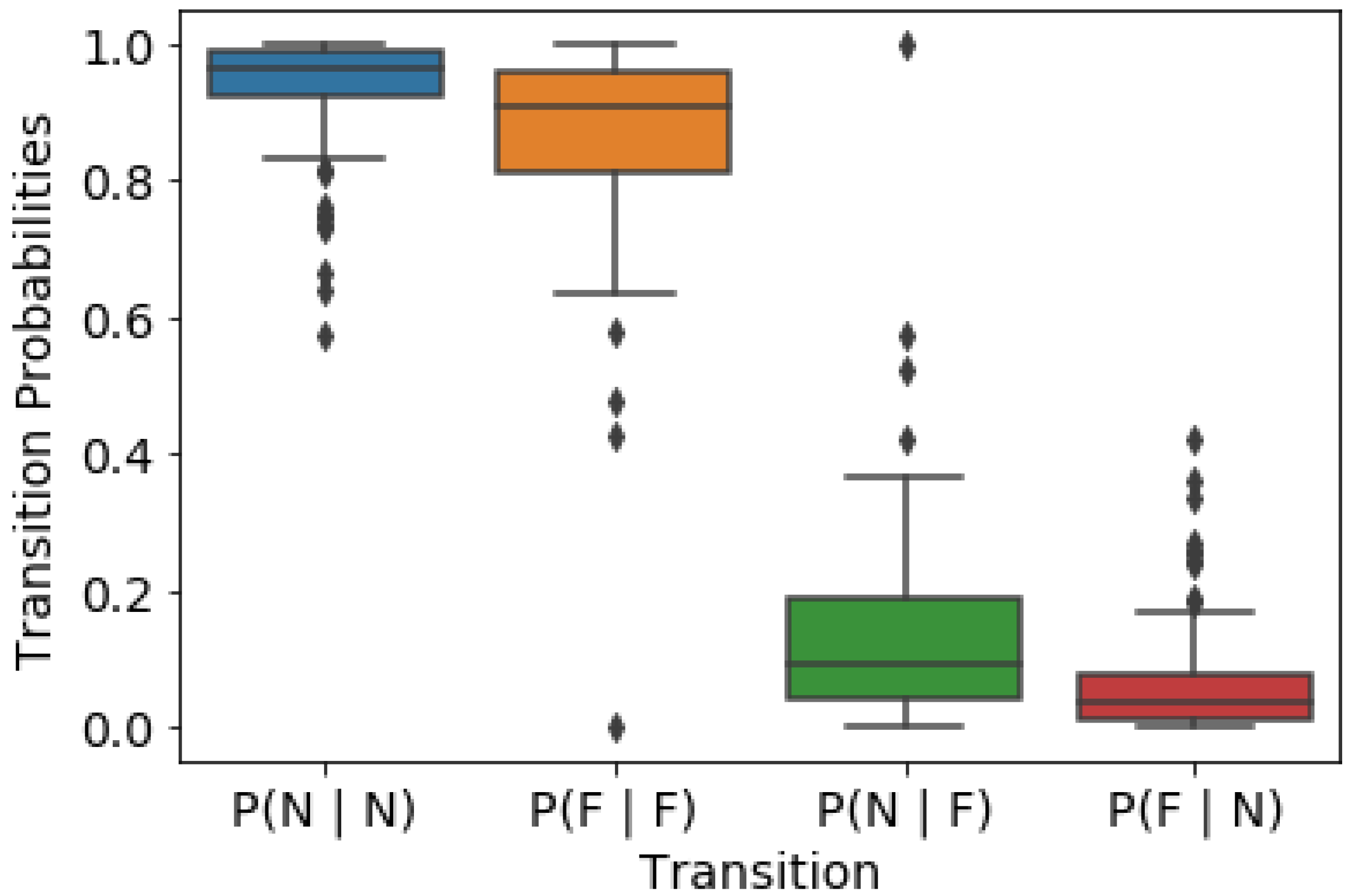
A total of 104 PV-HMM models were trained as part of this analysis. The transition probabilities evaluated from the Baum–Welch algorithm estimated
values (not shown) within the PV-HMM models demonstrate a preference towards maintaining a given state (
Figure 4). At all sites, when a system is currently in a normal state, it tends to stay normal in its next state. On average, this happens around 93.5% of the time across the sites (blue boxplot). This also indicates that there is a 6.5% probability of a failure in the next state given that the current state is normal (as shown in the red boxplot). On the other hand, we observe a lower probability of 87.1% of the next state being faulted when the current state is faulted (orange boxplot). By extension, this means that a 12.9% probability of returning to a normal state can be achieved given that the current state is faulted (green boxplot). The higher probability percentage from faulted to normal states (vs. normal to faulted) could reflect the site operators’ motivation to fix issues quickly to maintain as large an energy output as possible to maximize production.
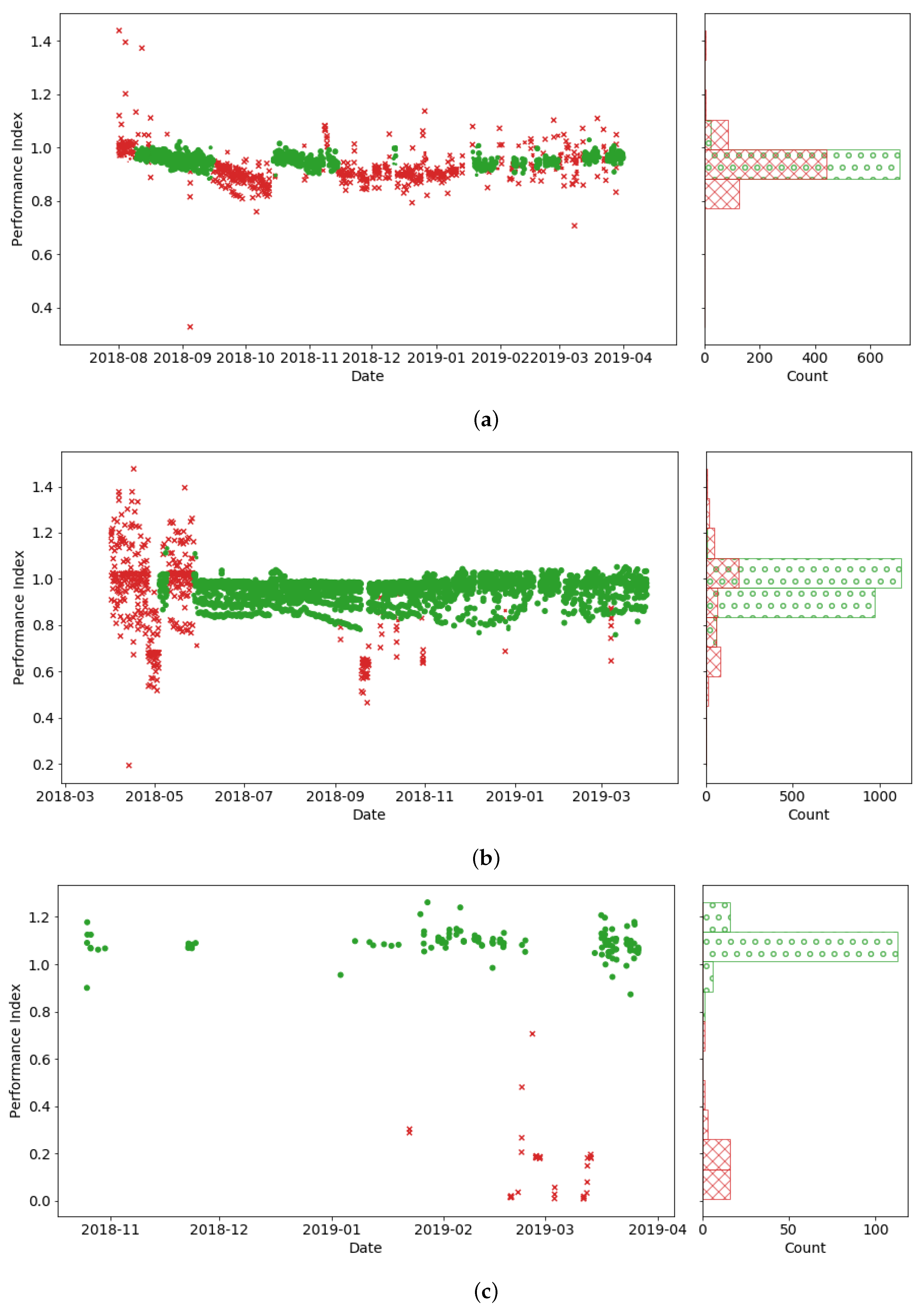
An evaluation of specific sites indicates that the PV-HMMs capture faulted states to also consider signatures related to heteroskedasticity (i.e., heterogeneous variance) as well as changes in mean values. For example, there is a general decline in PI mean values for one site in October 2018 that is flagged (in red) as faulted by the PV-HMM (
Figure 5a). No O&M tickets were observed at this site, so the general decline in PI could reflect environmental stressors that resolved on their own (e.g., snow that melted or soiling removed by rain). Values greater than one PI could reflect under-estimations of expected energy values that arise from irradiance or other sensor errors. Additional faulted states were also identified by the PV-HMM a few months later, capturing high variances in PI. Some sites, however, had more variable PI values in general. Even in such conditions, the PV-HMM was able to recognize faulted conditions (
Figure 5b). Finally, in contrast to ML methods which require long periods of data [
32], PV-HMMs can be trained on site data with as few as 170 data points (
Figure 5c).
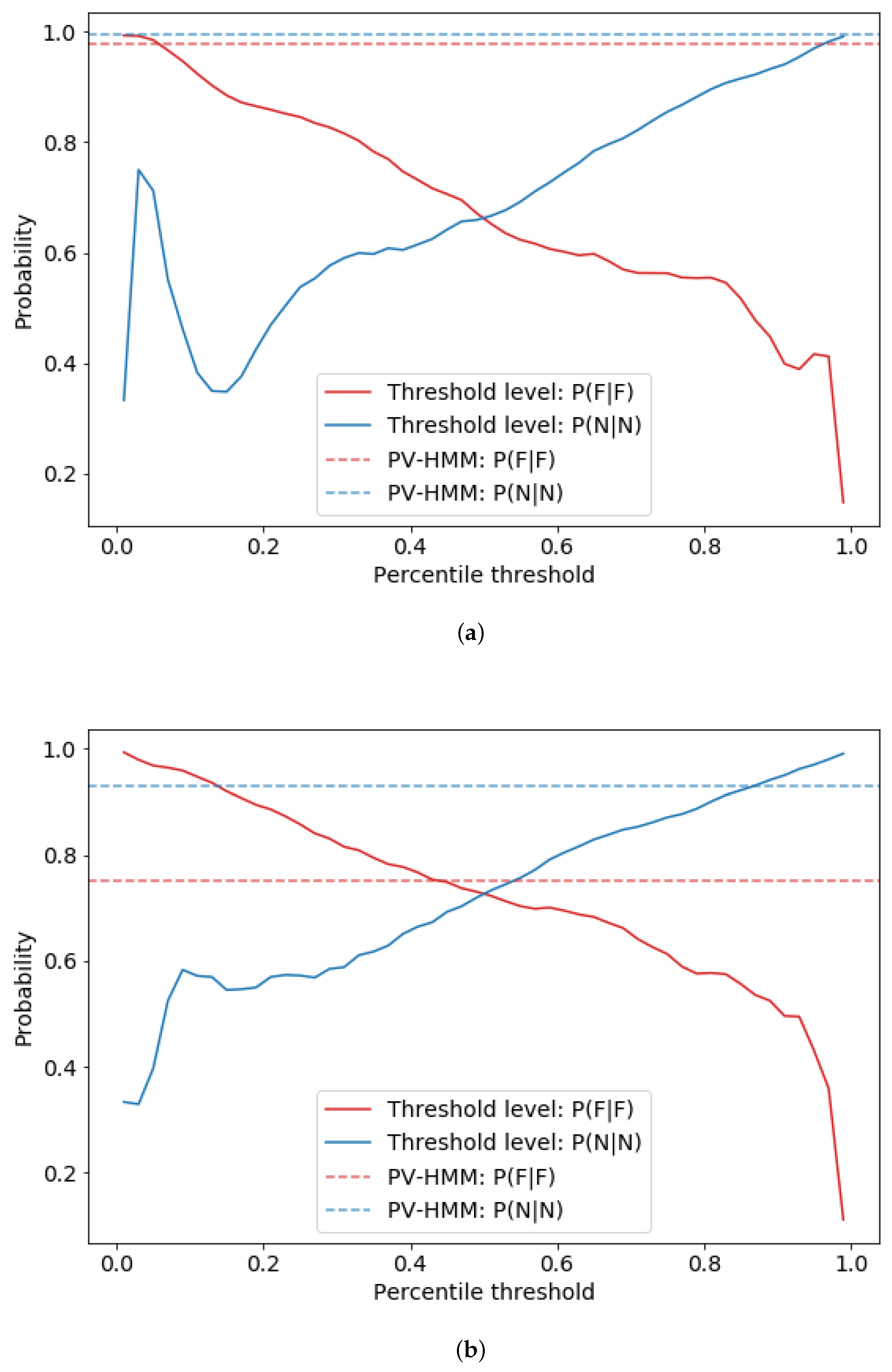
TL comparisons generally show that percentile thresholds between 0.80 to 0.98 align with PV-HMM transition probabilities for normal states given that a previous state is also normal (see examples in
Figure 6). For faulted to faulted PV-HMM transition probabilities, associated percentile thresholds generally range between 0.18 to 0.42. In addition to the general TL ranges, the site-level plots also highlight the general sensitivity of failure probabilities to specific thresholds, with many sites exhibiting a non-monotonic trend across different percentiles. Furthermore, a lack of ground truth with threshold levels, a common issue with TLs [
30], does not provide a complete evaluation for the performance of PV-HMMs.
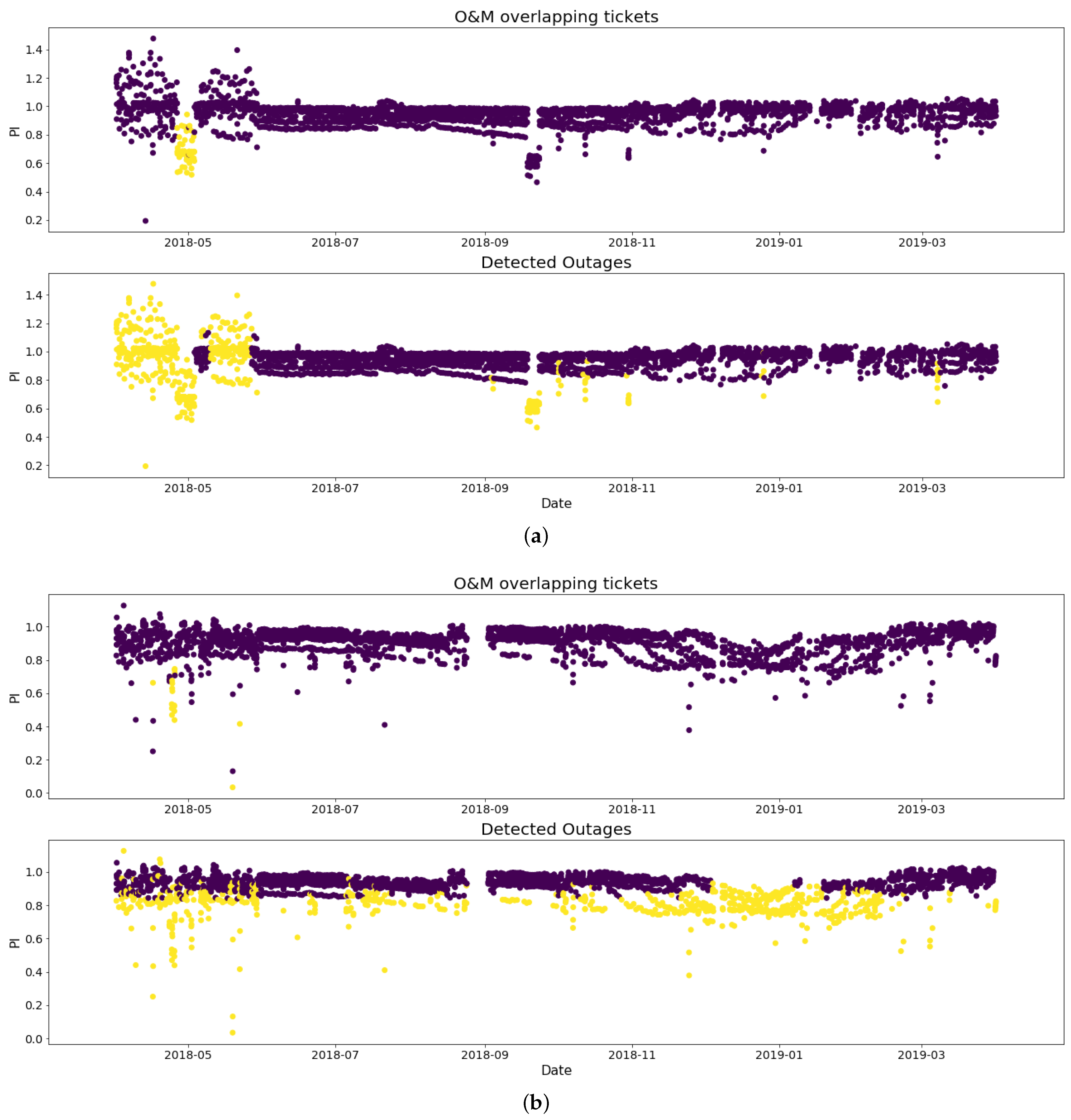
Therefore, to validate faulted states, precision metrics were calculated for each model (i.e., each site) using associated O&M tickets observed at each site. The calculations demonstrate high precision between the two datasets (median of 82.4% across the sites). This indicates that most of the periods with active O&M tickets were indeed flagged as detected faults by the PV-HMM. Site-level evaluations provide additional insights. For example, we see a deviation in performance identified by the PV-HMM that was missing in the O&M tickets (e.g., April 2018 and October 2018) (
Figure 7a). Looking at another system (
Figure 7b), the PV-HMM is able to capture more anomalies than identified by O&M tickets, including a notable dip in performance in December 2019. These examples highlight the strengths of the unsupervised learning pursued by PV-HMMs for detecting failures that could be targetted by O&M activities to improve overall site performance.
However, there are limitations in this analysis driven by a lack of ground truth that impacts all field-based PV failure methods. Additional data (across time and geographies) may be useful for comparing predictions to observations in the field. Such insights may also support increased coupling of production and O&M activities to automatically generate O&M tickets when faults are predicted through PV-HMMs. For example, the detected fault states from the PV-HMM also output an associated probability of class, which is used in the Viterbi algorithm to determine the states. Using bootstrapping techniques, these output probabilities can then be associated with confidence bounds that can be used to trigger generation of maintenance review activities in real time. Additionally, having ground truth data may aid the maximization of PV-HMM accuracy by extending the GMM emission density to incorporate specific exogenic covariates (e.g., weather conditions) whose effects on PV systems’ states can be explicitly quantified. The inclusion of these covariates may also provide insight into local conditions that prioritize maintenance activities (e.g., ignoring soiling and snow events). Future analyses may also consider building hierarchical PV-HMMs that take advantage of asset-level data to further support maintenance responses.
As noted above, the PV-HMM leveraged the Viterbi algorithm to calculate the most probable path of the PI into the future as a way to label normal vs. faulted states. These predictions, which were derived from each site’s transition and emission profile alone, could be extended into the future to support predictive failure modeling and associated maintenance activities. Although predictive maintenance is common in other industries, general implementation in PV has been limited, in part due to the lack of site-level demonstrations [
33]. New methods are needed to effectively quantify cost savings that could arise from predictive maintenance activities. However, solutions will only be successful if they go beyond looking at failure signatures for individual assets (current state of the art; [
34]) to consider signatures at the site level (where data are often analyzed). The use of PI as the sole input into the PV-HMM reduces the data requirements for the analysis. Future work should also consider incorporating these methods into open-source package distributions, such as
pvOps [
35], to support ongoing research and application testing of these statistical techniques.


