
Stochastic Modeling of Renewable Energy Sources for Capacity Credit Evaluation


Abstract
1. Introduction
2. Methodology and Data
2.1. Capacity Credit Evaluation of RE Power Plants
- is the time to failure or the duration of the generating unit availability;
- is the time to repair or the duration of the generating unit unavailability;
- is a random value with a uniform distribution in [0, 1];
- is a random value with a standard normal distribution;
- is the failure rate of each generating unit in a two-state Markov model;
- is the average repair time of each generating unit and equals 1/;
- is the repair rate of each generating unit in a two-state Markov model;
- is the variance of the repair time of each generating unit, modeled by 0.1r [71].
- is the load at time t;
- is the load forecast at time t;
- is the variance of load forecast error, modeled by [73];
- is a standard normally distributed random number, .
- is the duration that the total power output of all units is less than load ;
- is the total considering period.
2.2. Stochastic Model of RE Generation
2.2.1. Wind
- Wind Speed Model
- is the variance of historical hourly wind speed at hour
- is the Wiener process, where ;
- is a standard normally distributed random number.
- 2.
- Wind Operation Model
- Cut-in wind speed : At this wind speed, a wind turbine starts moving leading to a generator gradually generating electrical power;
- Maximum rotor efficiency wind speed: This is a range of wind speed between the cut-in and a rated wind speed where power output depends on wind speed value;
- Rated or nominal output wind speed : Once the wind speed reaches this level, the generator comes to its maximum capacity in generating electrical power;
- Cut-out wind speed : It is the maximum wind speed at which the turbine is allowed to be operated. At this level, wind blades are set to be aligned with a wind flow to prevent the turbine from moving to avoid damage from excessively high wind speed.
- is the rated power (W);
- is the efficiency of a corresponding converter.
2.2.2. Solar PV
- Solar Irradiance and Ambient Temperature Models
- is the variance of historical hourly solar irradiance at hour
- is the variance of historical hourly ambient temperature at hour ;
- is a standard normally distributed random number which is correlated to
- is a standard normally distributed random number which is correlated to
- 2.
- Copula Application for Joint Probability Distribution
- is a standard normal distribution of
- is a standard normal distribution of .
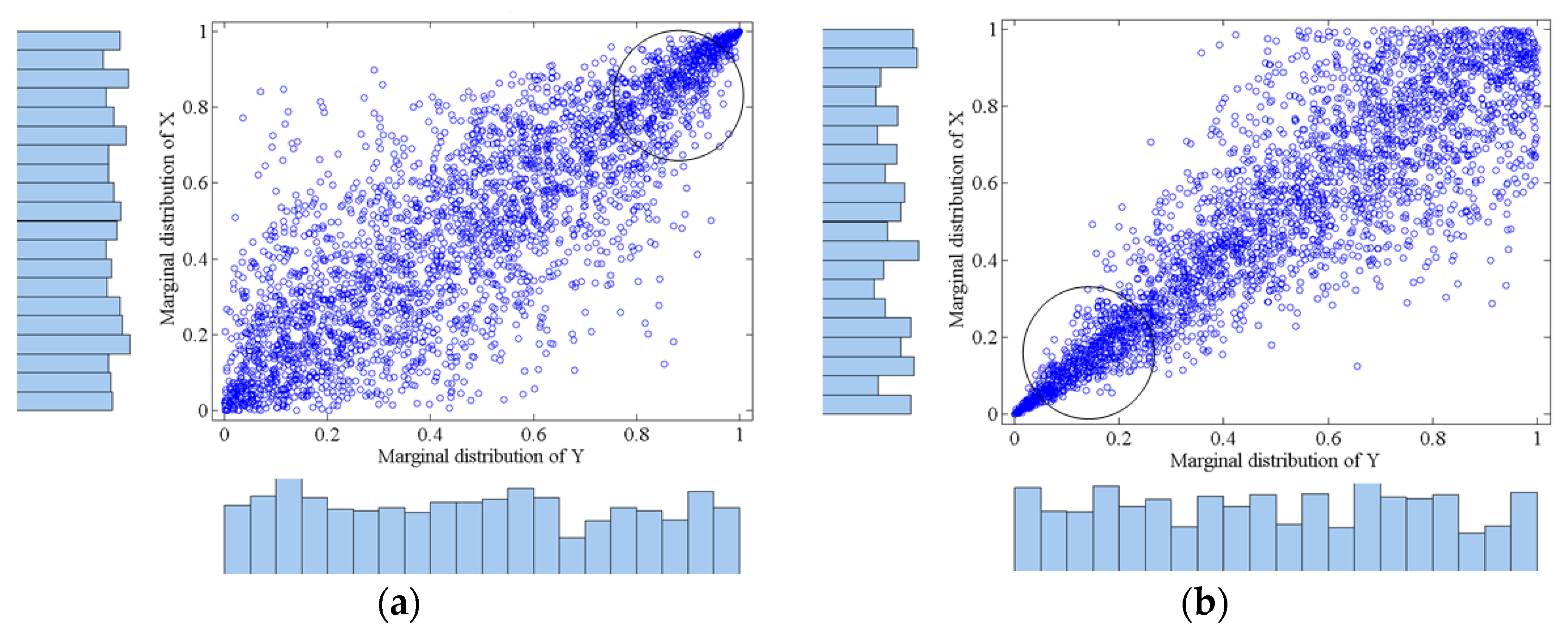
- Gumbel copula exhibits strong correlation at high values, which correspond to the nature of solar when high solar irradiance comes with a high ambient temperature. However, at the low values, Gumbel copula has weak correlation;
- Clayton copula has strong left tail dependence which captures the nature of solar when low solar irradiance comes with low ambient temperature.
- 3.
- Solar PV Operation Model
- is the rated power of solar PV (W);
- is the solar irradiance at the standard test condition (1000 W/m2);
- is the temperature coefficient which is −0.005 to −0.003;
- is the solar cell temperature ;
- is the standard test condition temperature (25 );
- is the ambient temperature ;
- is the nominal operating cell temperature (46 );
- is efficiency of a corresponding converter.
2.2.3. Small Hydro
- Mass Flow Rate Model
- 2.
- Small Hydro Operation Model
- is the acceleration due to gravity at the surface of the earth (9.81 m/s2);
- is the head or falling height (m);
- is the efficiency of hydro generation.
2.2.4. Bio-Based Power and MSW
- Feedstock Availability Model
- is the feedstock availability of the considered fuel type at time
- is the location parameter;
- is the shape parameter;
- is the scale parameter.
- 2.
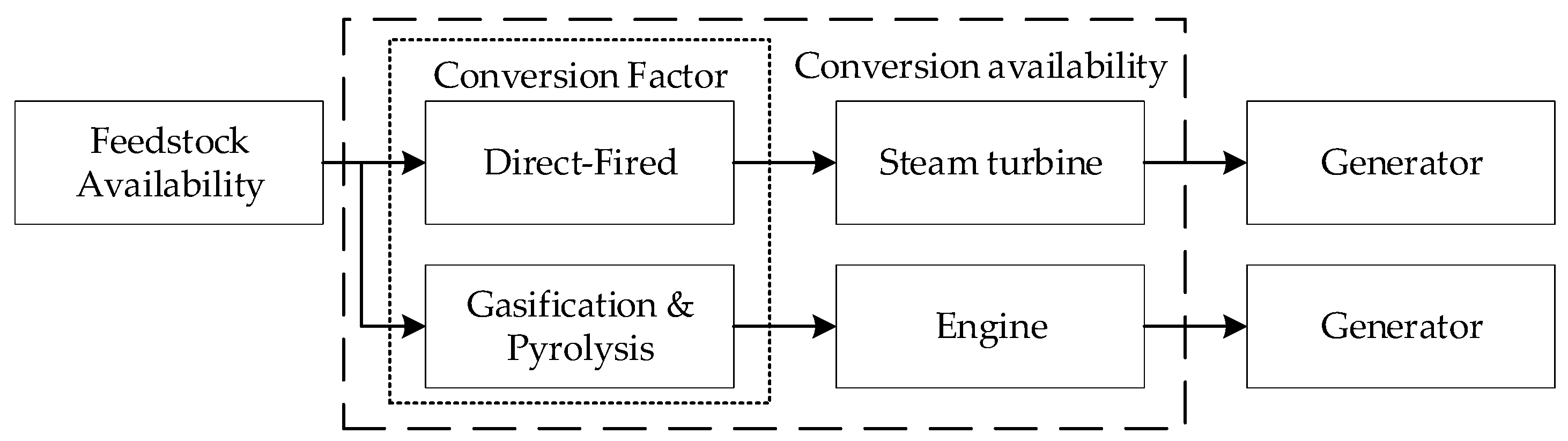
- Bio-based Conversion Model
- Biomass Operation Model
- B.
- Biogas Operation Model
- C.
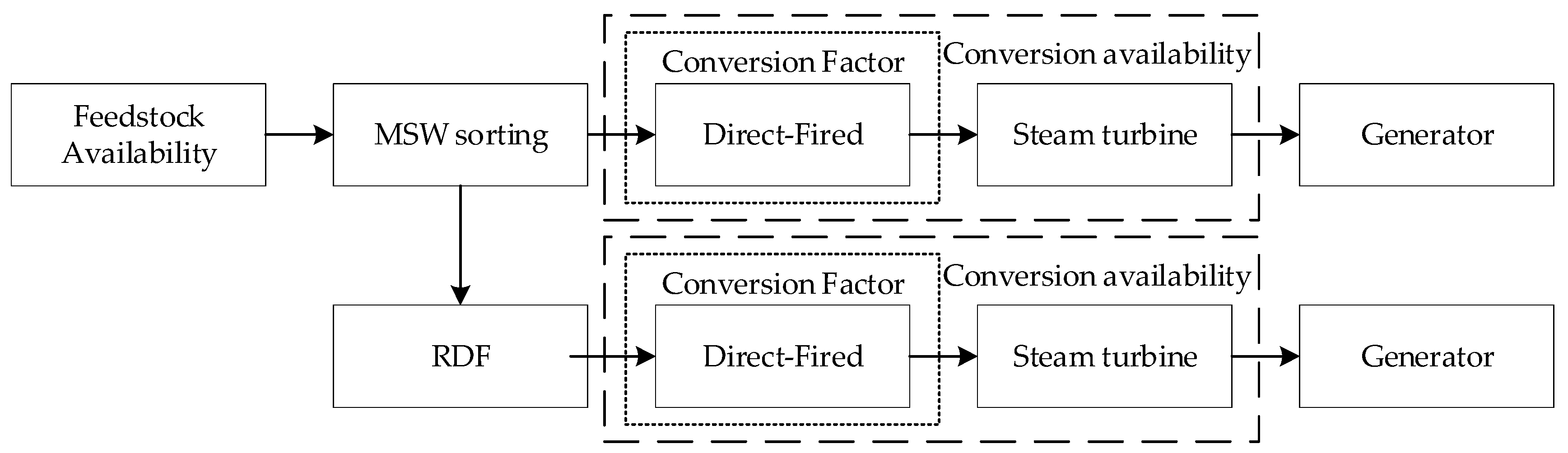
- MSW Operation Model
- 3.
- System Availability
- is the conversion factor of fuel to power (%);
- is the availability of biogas or biomass system, which is either 0 or 1;
- is the installed capacity of biomass or biogas generation.
- is the waste matter that can be turned into electricity;
- is the yield of RDF from waste matter that can be turned into electricity;
- is the conversion factor of the RDF;
- is the conversion factor of the remaining sorted MSW;
- is the availability of the MSW system, which is either 0 or 1.
2.3. Data and Assumptions
2.3.1. Generation System and Load
2.3.2. RE Generation Data
- Wind: The wind data used in the wind generation model include the monthly average wind speed, hourly mean, and standard deviation of wind speed at each hour, as shown in Figure 19. The cut-in ( ), rated (), and cut-out () wind speed are given as 2.8, 12.5, and 23 m/s, respectively. The efficiency of a corresponding converter () is 98%.
- Solar PV: The solar data used for the solar PV generation model consist of the hourly mean and standard deviation of solar irradiance and ambiance temperature for summer, rainy, and winter season, as shown in Figure 20. The correlations of solar irradiance and ambient temperature during 7 AM–1 PM and 2–6 PM are given as Gumbel copula and Frank copula, respectively. The temperature coefficient () is –0.0035 and the nominal operating cell temperature () is 46 °C. The efficiency of a corresponding converter () is 98%.
- Small hydro: Water flow rate of small hydro generation is given as a normal distribution with the average water flow rate () of 50 liters/s and standard deviation () of 25% of the mean. The rated power output () of the generator is 37 kW with the rated water flow rate () of 60 l/s. The probability distribution function of water flow rate is shown in Figure 21a.
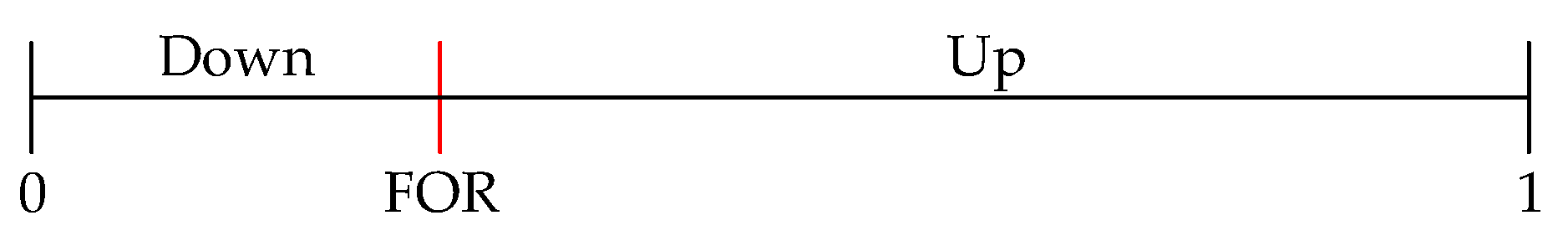
- Biomass: The average feedstock availability of biomass in Thailand is assumed to be 60–70% of the installed capacity. Given that, the feedstock availability is represented by the Weibull distribution with calibrated location, shape, and scale parameters of 30, 2.48, and 45.2, respectively. The CF of the biomass generation system is expressed by the normal distribution with a mean of 95% and a standard deviation of 1% of the mean. The AV of conversion system is assumed to be equivalent to the forced outage rate (FOR) of 10%. The probability distribution function of feedstock availability and biomass conversion factor are shown in Figure 21b,c, respectively.
- Biogas: In Thailand, it is assumed that the average ratio of CH4 in biogas production is 55% [91] and is modeled by the Weibull distribution with location, shape, and scale parameters of 0, 25, and 55, respectively. With this CH4 ratio, the CF of biogas generation is then computed from the linear transformation that a CH4 of 55% equals the conversion factor of 100% or CF = CH4/0.55. The AV of the conversion system is assumed to be equivalent to the FOR of 15%. The probability distribution function of biogas production and biogas conversion factor are shown in Figure 21d,e, respectively.
- MSW: The waste matter that can be turned to electricity is expressed by the Weibull distribution with the location, shape, and scale parameters of 0.7, 12, and 90, respectively. With this distribution, the waste used for electricity generation is 90% on average. The yield of RDF is represented by the normal distribution with a mean of 20% and a standard deviation of 1% of the mean. Because RDF largely consists of combustible components, the is given at a constant of 100%, while, for non-RDF, the is described by the normal distribution with a mean of 95% and standard deviation of 1% of the mean. The AV of conversion system is assumed to be equivalent to the FOR of 10%. The probability distribution function of waste used for electricity generation, a yield of RDF, and non-RDF conversion factor are shown in Figure 21f,g,h, respectively.
3. Results and Discussions
- Wind: Due to the continuous power output of wind generation, the capacity credits throughout the day, during the day peak period (2–3 PM), and night peak period (7–8 PM) are slightly different, which are in the range of 9.57–12.96%. This difference is caused by the difference in average hourly wind speed and noise in the proposed wind generation model used in this study since wind power generation is modeled hourly.
- Solar PV: The average capacity credits throughout the day is lower than the capacity credit during the day peak period (2–3 PM) since solar PV generation can only produce electricity during daytime (7 AM–6 PM). During the peak load period, the existence of solar PV generation can significantly enhance the LOLE. On the other hand, solar PV generation has no capacity credit during the night peak period.
- Small hydro: The average capacity credits of small hydro generation throughout the day, during the day peak period, and during the night peak period are slightly different, which are in the range of 64.45–73.05%. Since small hydro generations are modeled daily, the difference between each time of day is caused by the LOLE of the system during that period.
- Biomass: Since the power output of biomass generation is consistent, its average capacity credits throughout the day, during the day peak period, and during the night peak period are not significantly different, which are in the range of 57.57–67.38%. Due to the lack of solar PV generation during the night peak period, the LOLE is more sensitive to other types of RE generation that can supply electricity during night peak period, especially during the peak period when LOLE is quite high. Thus, the capacity credit of biomass generation during the night peak period is slightly higher.
- Biogas: Due to the nearly identical generation model, the capacity credit trend of biogas generation throughout the day, during the day peak period, and during the night peak period are almost identical to that of biomass. However, the values, which are in the range of 49.02–56.25%, are lower than those of biomass generation since the biogas generation model has a higher uncertainty from a biogas production and availability of conversion system. It was also found that the capacity credit of the biogas generation during the night peak period is slightly higher than the day peak period.
- MSW: The capacity credit trends of MSW generation for all different considered periods resemble those of biomass generation since both of them have similar generation models, except for the uncertainty of waste matter which can be turned into electricity and the ratio between RDF and non-RDF. These uncertainties lead to slightly lower capacity credits of MSW generation, which are in the range of 52.95–59.96%.
4. Conclusions
Author Contributions
Funding
Institutional Review Board Statement
Informed Consent Statement
Data Availability Statement
Conflicts of Interest
Appendix A. Detail Proof of the Proposed Noise Model
- is a variance of hourly average value at hour
- is a Wiener process equal to ;
- is a standard normally distributed random value.
- is a noise at equal to 0;
- is a noise at any considered time .
Appendix B. Generation System Data

| Fuel Type | Number (Unit) | Total Capacity (MW) | Capacity Factor | (f/yr) | (f/yr) |
|---|---|---|---|---|---|
| Lignite | 10 | 2180 | 85 | 7.617 | 87.6 |
| Bituminous | 5 | 1566.5 | 60–85 | 7.617 | 87.6 |
| Natural gas | 58 | 20,793.3 | 60–80 | 7.617 | 87.6 |
| Diesel | 1 | 4.4 | 20 | 2.98 | 146 |
| Oil | 1 | 315 | 40 | 7.617 | 87.6 |
| HVDC | 1 | 300 | 0 | 0 | 1 |
| Hydro | 17 | 3423.7 | 19.72 | 7.964 | 58.4 |
| Import hydro | 2 | 340 | 52 | 7.964 | 58.4 |
| Wind | 1 | 2.5 | 20 | FOR ≈ 0% | |
| Solar PV | 1 | 2 | 18 | FOR ≈ 0% | |
| Biomass | 8 | 281 | 74 | FOR = 10% | |
| Biogas | 2 | 12 | 74 | FOR = 15% | |
| MSW | 1 | 11 | 74 | FOR = 10% | |
Appendix C. Simulated Power Output of RE Generation Unit

References
- REN21. Renewables 2020 Global Status Report. Available online: https://www.ren21.net/gsr-2020/ (accessed on 12 June 2022).
- Erdiwansyah, E.; Mahidin, M.; Mamat, R.; Sani, M.S.M.; Khoerunnisa, F.; Kadarohman, A. Target and demand for renewable energy across 10 ASEAN countries by 2040. Electr. J. 2019, 32, 106670. [Google Scholar] [CrossRef]
- Van Soest, H.L.; den Elzen, M.G.J.; van Vuuren, D.P. Net-zero emission targets for major emitting countries consistent with the Paris Agreement. Nat. Commun. 2021, 12, 2140. [Google Scholar] [CrossRef]
- IEA. Renewables 2021. Available online: https://www.iea.org/reports/renewables-2021 (accessed on 12 June 2022).
- Diewvilai, R.; Audomvongseree, K. Possible Pathways toward Carbon Neutrality in Thailand’s Electricity Sector by 2050 through the Introduction of H2 Blending in Natural Gas and Solar PV with BESS. Energies 2022, 15, 3979. [Google Scholar] [CrossRef]
- Scholtz, A. The European Green Deal & Fit for 55. Available online: https://assets.kpmg/content/dam/kpmg/xx/pdf/2021/11/green-deal-and-fit-for-55-slip-sheet_v5_web.pdf (accessed on 12 June 2022).
- Min, H. China’s Net Zero Future. Available online: https://climatechampions.unfccc.int/chinas-net-zero-future/ (accessed on 12 June 2022).
- Zhao, C.; Ju, S.; Xue, Y.; Ren, T.; Ji, Y. China’s energy transitions for carbon neutrality: Challenges and opportunities. Carbon Neutrality 2022, 1, 7. [Google Scholar] [CrossRef]
- Photovoltaic Power Systems Programme; International Energy Agency. Trends in PV Applications 2021. Available online: https://iea-pvps.org/trends_reports/trends-in-pv-applications-2021/ (accessed on 12 June 2022).
- Feldman, D.; Ramasamy, V.; Fu, R.; Ramdas, A.; Desai, J.; NREL. U.S. Solar Photovoltaic System and Energy Storage Cost Benchmark: Q1 2020. Available online: https://www.nrel.gov/docs/fy21osti/77324.pdf (accessed on 12 June 2022).
- IRENA. The Power to Change: Solar and Wind Cost Reduction Potential to 2025. Available online: https://www.irena.org/publications/2016/Jun/The-Power-to-Change-Solar-and-Wind-Cost-Reduction-Potential-to-2025 (accessed on 12 June 2022).
- Lazard Lazard’s Levelized Cost of Energy Analysis—Version 14.0. Available online: https://www.lazard.com/media/451419/lazards-levelized-cost-of-energy-version-140.pdf (accessed on 12 June 2022).
- Csereklyei, Z.; Qu, S.; Ancev, T. Are electricity system outages and the generation mix related? Evidence from NSW, Australia. Energy Econ. 2021, 99, 105274. [Google Scholar] [CrossRef]
- IRENA. Renewable Power Generation Costs in 2020. Available online: https://www.irena.org/publications/2021/Jun/Renewable-Power-Costs-in-2020 (accessed on 12 June 2022).
- IRENA. Biomass for Power Generation. Available online: https://www.irena.org/-/media/Files/IRENA/Agency/Publication/2012/RE_Technologies_Cost_Analysis-BIOMASS.pdf (accessed on 12 June 2022).
- Liu, Z.; Li, X. Analysis of the investment cost of typical biomass power generation projects in China. In Proceedings of the 2016 International Conference on Education, Management Science and Economics, Singapore, 26–28 December 2016. [Google Scholar]
- Statista Average Installation Cost for Bioenergy Plants Worldwide from 2010 to 2018 (in U.S. Dollars per Kilowatt). Available online: https://www.statista.com/statistics/799356/global-bioenergy-installation-cost-per-kilowatt/ (accessed on 12 June 2022).
- Patro, E.R.; Kishore, T.S.; Haghighi, A.T. Levelized cost of electricity generation by small hydropower projects under clean development mechanism in India. Energies 2022, 15, 1473. [Google Scholar] [CrossRef]
- Capitanescu, F. Evaluating reactive power reserves scarcity during the energy transition toward 100% renewable supply. Electr. Power Syst. Res. 2021, 190, 106672. [Google Scholar] [CrossRef]
- Kishore, T.S.; Patro, E.R.; Harish, V.S.K.V.; Haghighi, A.T. A comprehensive study on the recent progress and trends in development of Small hydropower projects. Energies 2021, 14, 2882. [Google Scholar] [CrossRef]
- Sharma, N.K.; Sood, Y.R. A comprehensive analysis of strategies, policies and development of hydropower in India: Special emphasis on small hydro power. Renew. Sustain. Energy Rev. 2013, 18, 460–470. [Google Scholar] [CrossRef]
- Michael, T. 2—Environmental and social impacts of waste to energy (WTE) conversion plants. In Waste to Energy Conversion Technology; Woodhead Publishing: Sawston, UK, 2013; pp. 15–28. [Google Scholar]
- Xiao, H.; Li, Z.; Jia, X.; Ren, J. Chapter 2—Waste to energy in a circular economy approach for better sustainability: A comprehensive review and SWOT analysis. In Waste-to-Energy; Academic Press: Cambridge, MA, USA, 2020; pp. 23–43. [Google Scholar]
- Pattanapongchai, A.; Limmeechokchai, B. The co-benefits of biogas from the palm oil industry in long-term energy planning: A least-cost biogas upgrade in Thailand. Energy Sources Part B Econ. Plan. Policy 2014, 9, 360–373. [Google Scholar] [CrossRef]
- Silaen, M.; Taylor, R.; Bößner, S.; Anger-Kraavi, A.; Chewpreecha, U.; Badinotti, A.; Takama, T. Lessons from Bali for small-scale biogas development in Indonesia. Environ. Innov. Soc. Transit. 2020, 35, 445–459. [Google Scholar] [CrossRef]
- ASEAN Strategy on Sustainable Biomass Energy for Agriculture Communities and Rural Development in 2020–2030. Available online: https://greenenergyasean.com/en/strategy/asean-strategy-on-sustainable-biomass-energy-for-agriculture-communities-and-rural-development-in-2020-2030/8 (accessed on 12 June 2022).
- Beyz, J.; Yusta, J.M. The effects of the high penetration of renewable energies on the reliability and vulnerability of interconnected electric power systems. Reliab. Eng. Syst. Saf. 2021, 215, 107881. [Google Scholar] [CrossRef]
- Navia, M.; Orellana, R.; Zaráte, S.; Villazón, M.; Balderrama, S.; Quoilin, S. Energy transition planning with high penetration of variable renewable energy in developing countries: The case of the Bolivian interconnected power system. Energies 2022, 15, 968. [Google Scholar] [CrossRef]
- Kaushik, E.; Mahela, O.P.; Khan, B.; El-Shahat, A. Comprehensive overview of power system flexibility during the scenario of high penetration of renewable energy in utility grid. Energies 2022, 15, 516. [Google Scholar] [CrossRef]
- Dong, L. Evaluation of electricity supply sustainability and security: Multi-criteria decision analysis approach. J. Clean. Prod. 2018, 172, 438–453. [Google Scholar] [CrossRef]
- Talari, S.; Shafie-khah, M.; Osório, G.J.; Aghaei, J.; Catalão, J.P.S. Stochastic modelling of renewable energy sources from operators’ point-of-view: A survey. Renew. Sustain. Energy Rev. 2018, 81, 1953–1965. [Google Scholar] [CrossRef]
- Cui, D.; Xu, F.; Ge, W.; Huang, P.; Zhou, Y. A coordinated dispatching model considering generation and operation reserve in wind power-photovoltaic-pumped storage system. Energies 2020, 13, 4834. [Google Scholar] [CrossRef]
- Firouzi, M.; Samimi, A. Abolfazl Salami Reliability evaluation of a composite power system in the presence of renewable generations. Reliab. Eng. Syst. Saf. 2022, 222, 108396. [Google Scholar] [CrossRef]
- Yang, X.; Yang, Y.; Liu, Y.; Deng, Z. A reliability assessment approach for Electric power systems considering wind power uncertainty. IEEE Access 2020, 8, 12467–12478. [Google Scholar] [CrossRef]
- Garver, L.L. Effective load carrying capability of generating units. IEEE Trans. Power Appar. Syst. 1966, 8, 910–919. [Google Scholar] [CrossRef]
- Wang, S.; Zheng, N.; Bothwell, C.D.; Xu, Q.; Kasina, S.; Hobbs, B.F. Crediting variable renewable energy and energy storage in capacity markets: Effects of unit commitment and storage operation. IEEE Trans. Power Syst. 2022, 37, 617–628. [Google Scholar] [CrossRef]
- Madaeni, S.H.; Sioshansi, R. Comparison of Capacity Value Methods for Photovoltaics in the Western United States. Available online: https://www.nrel.gov/docs/fy12osti/54704.pdf (accessed on 12 June 2022).
- Chen, F.; Li, F.; Feng, W.; Wei, Z.; Cui, H.; Liu, H. Reliability assessment method of composite power system with wind farms and its application in capacity credit evaluation of wind farms. Electr. Power Syst. Res. 2019, 166, 73–82. [Google Scholar] [CrossRef]
- Diewvilai, R.; Audomvongseree, K. Generation expansion planning with energy storage systems considering renewable energy generation profiles and full-year hourly power balance constraints. Energies 2021, 14, 5733. [Google Scholar] [CrossRef]
- Söder, L.; Tómasson, E.; Estanqueiro, A.; Flynn, D.; Hodge, B.-M.; Kiviluoma, J.; Korpås, M.; Neau, E.; Couto, A.; Pudjianto, D.; et al. Review of wind generation within adequacy calculations and capacity markets for different power systems. Renew. Sustain. Energy Rev. 2020, 119, 109540. [Google Scholar] [CrossRef]
- Milligan, M.; Porter, K. The capacity value of wind in the United States: Methods and implementation. Electr. J. 2006, 19, 91–99. [Google Scholar] [CrossRef]
- Madaeni, S.H.; Sioshansi, R.; Denholm, P. Comparing capacity value estimation techniques for photovoltaic solar power. IEEE J. Photovolt. 2013, 3, 407–415. [Google Scholar] [CrossRef]
- Jorgenson, J.; Awara, S.; Stephen, G.; Mai, T. Comparing Capacity Credit Calculations for Wind: A Case Study in Texas. Available online: https://www.nrel.gov/docs/fy21osti/80486.pdf (accessed on 12 June 2022).
- Dragoon, K.; Dvortsov, V. Z-method for power system resource adequacy applications. IEEE Trans. Power Syst. 2006, 21, 982–988. [Google Scholar] [CrossRef]
- Zhou, E.; Cole, W.; Frew, B. Valuing variable renewable energy for peak demand requirements. Energy 2018, 165, 499–511. [Google Scholar] [CrossRef]
- Milligan, M.; Parsons, B. A comparison and case study of capacity credit algorithms for wind power plants. Wind Eng. 1999, 23, 159–166. [Google Scholar]
- Energy Policy and planning Office. Summary Of Thailand Power Development plan (PDP2010:Revision 3). Available online: https://www.erc.or.th/ERCWeb2/Upload/Document/PDP2010-Rev3-Cab19Jun2012-E.pdf (accessed on 31 August 2021).
- Ministry of Energy. Thailand’s Power Development Plan (PDP). 2018. Available online: http://www.eppo.go.th/images/POLICY/PDF/PDP2018.pdf (accessed on 16 January 2022).
- NERC. 2021 Long-Term Reliability Assessment. Available online: https://www.nerc.com/pa/RAPA/ra/Reliability%20Assessments%20DL/NERC_LTRA_2021.pdf (accessed on 12 June 2022).
- Gerres, T.; Ávila, J.P.C.; Martínez, F.M.; Abbad, M.R.; Arín, R.C.; Miralles, Á.S. Rethinking the electricity market design: Remuneration mechanisms to reach high RES shares. Results from a Spanish case study. Energy Policy 2019, 129, 1320–1330. [Google Scholar] [CrossRef]
- MTIE. The 9th Basic Plan for Long-Term Electricity Supply and Demand. Available online: http://www.motie.go.kr/motie/ne/presse/press2/bbs/bbsView.do?bbs_seq_n=163670&bbs_cd_n=81 (accessed on 12 June 2022).
- Ministry of Energy. Thailand’s Power Development Plan (PDP) 2018 Rev. 1. Available online: https://policy.asiapacificenergy.org/node/4347/portal (accessed on 31 August 2021). (In Korean)
- Byers, C.; Botterud, A. Additional capacity value from synergy of variable renewable energy and energy storage. IEEE Trans. Sustain. Energy 2020, 1, 1106–1109. [Google Scholar] [CrossRef]
- Zhu, Z.; Wang, X.; Jiang, C.; Wang, L.; Gong, K. Multi-objective optimal operation of pumped-hydro-solar hybrid system considering effective load carrying capability using improved NBI method. Int. J. Electr. Power Energy Syst. 2021, 129, 106802. [Google Scholar] [CrossRef]
- Amelin, M. Comparison of capacity credit calculation methods for conventional power plants and wind power. IEEE Trans. Power Syst. 2009, 24, 685–691. [Google Scholar] [CrossRef]
- Haslett, J.; Diesendorf, M. The capacity credit of wind power: A theoretical analysis. Sol. Energy 1981, 26, 391–401. [Google Scholar] [CrossRef]
- Cai, J.; Xu, Q. Capacity credit evaluation of wind energy using a robust secant method incorporating improved importance sampling. Sustain. Energy Technol. Assess. 2021, 43, 100892. [Google Scholar] [CrossRef]
- Madaeni, S.H.; Sioshansi, R.; Denholm, P. Estimating the capacity value of concentrating solar power plants: A case study of the southwestern United States. IEEE Trans. Power Syst. 2012, 27, 1116–1124. [Google Scholar] [CrossRef]
- Verdejo, H.; Awerkin, A.; Kliemann, W.; Becker, C. Modelling uncertainties in electrical power systems with stochastic differential equations. Int. J. Electr. Power Energy Syst. 2019, 113, 322–332. [Google Scholar] [CrossRef]
- Loukatou, A.; Howell, S.; Johnson, P.; Duck, P. Stochastic wind speed modelling for estimation of expected wind power output. Appl. Energy 2018, 228, 1328–1340. [Google Scholar] [CrossRef]
- Obukhov, S.; Ibrahim, A.; Davydov, D.Y.; Alharbi, T.; Ahmed, E.M.; Ali, Z.M. Modeling wind speed based on fractional ornstein-uhlenbeck process. Energies 2021, 14, 5561. [Google Scholar] [CrossRef]
- Wang, J.; Alshelahi, A.; You, M.; Byon, E.; Saigal, R. Integrative Density Forecast and Uncertainty Quantification of Wind Power Generation. IEEE Trans. Sustain. Energy 2021, 12, 1864–1875. [Google Scholar] [CrossRef]
- Arenas-López, J.P.; Badaoui, M. Stochastic modelling of wind speeds based on turbulence intensity. Renew. Energy 2020, 155, 10–22. [Google Scholar] [CrossRef]
- Arenas-López, J.P.; Badaoui, M. A Fokker–Planck equation based approach for modelling wind speed and its power output. Energy Convers. Manag. 2020, 222, 113152. [Google Scholar] [CrossRef]
- Iversen, E.B.; Morales, J.M.; Møller, J.K.; Madsen, H. Probabilistic forecasts of solar irradiance using stochastic differential equations. Environmetrics 2014, 25, 152–164. [Google Scholar] [CrossRef]
- Tran, V.L. Stochastic Models of Solar Radiation Processes. General Mathematics. Ph.D. Thesis, University of Orleans, Orleans, France, 2013. [Google Scholar]
- Politaki, D.; Alouf, S. Stochastic Models for Solar Power. In Proceedings of the EPEW 2017—European Performance Engineering Workshop, Berlin, Germany, 7–8 September 2017; pp. 282–297. [Google Scholar]
- Farahmand, M.Z.; Nazari, M.E.; Shamlou, S.; Shafie-khah, M. The simultaneous impacts of seasonal weather and solar conditions on PV panels electrical characteristics. Energies 2021, 14, 845. [Google Scholar] [CrossRef]
- EERE. Types of Hydropower Plants. Available online: https://www.energy.gov/eere/water/types-hydropower-plants (accessed on 12 June 2022).
- Shabani, N.; Sowlati, T. A hybrid multi-stage stochastic programming-robust optimization model for maximizing the supply chain of a forest-based biomass power plant considering uncertainties. J. Clean. Prod. 2016, 112, 3285–3293. [Google Scholar] [CrossRef]
- Naksrisuk, C.; Audomvongseree, K. Dependable capacity evaluation of wind power and solar power generation systems. ECTI Trans. Electr. Eng. Electron. Commun. 2013, 11, 58–66. [Google Scholar]
- Billinton, R.; Allan, R. Reliability Evaluation of Power Systems; Pitman Advanced Publishing Program: London, UK, 1984; ISBN 0273084852. [Google Scholar]
- Audomvongseree, K.; Yokoyama, A.; Verma, S.C.; Nakachi, Y. A Novel TRM Calculation Method by Probabilistic Concept. IEEJ Trans. Power Energy 2004, 124, 1400–1407. [Google Scholar] [CrossRef][Green Version]
- Billington, R.; Allan, R.N. Reliability Evaluation of Power Systems, 2nd ed.; Plenum Press: New York, NY, USA, 1996. [Google Scholar]
- Samorodnitsky, G.; Taqqu, M.S. Stable Non-Gaussian Random Processes: Stochastic Models with Infinite Variance, 1st ed.; Chapman & Hall: New York, NY, USA, 1994. [Google Scholar]
- Hassler, U. Stochastic Processes and Calculus: An Elementary Introduction with Applications, 1st ed.; Springer: Berlin/Heidelberg, Germany, 2016; ISBN 978-3319234274. [Google Scholar]
- Patel, M.R. Wind and Solar Power Systems: Design, Analysis, and Operation, 2nd ed.; CRC Press: Boca Raton, FL, USA, 2005. [Google Scholar]
- Chedid, R.; Akiki, H.; Rahman, S. A decision support technique for the design of hybrid solar-wind power systems. IEEE Trans. Energy Convers. 1998, 13, 76–83. [Google Scholar] [CrossRef]
- Ramírez, A.F.; Valencia, C.F.; Cabrales, S.; Ramírez, C.G. Simulation of photo-voltaic power generation using copula autoregressive models for solar irradiance and air temperature time series. Renew. Energy 2021, 175, 44–67. [Google Scholar] [CrossRef]
- Cherubini, U.; Luciano, E.; Vecchiato, W. Copula Methods in Finance, 1st ed.; Wiley: Chichester, UK, 2004; ISBN 978-0-470-86344-2. [Google Scholar]
- Depuru, S.R.; Mahankali, M. Performance Analysis of a Maximum Power Point Tracking Technique using Silver Mean Method. Adv. Electr. Electron. Eng. 2018, 16, 25–35. [Google Scholar] [CrossRef]
- Fuentes, M.; Nofuentes, G.; Aguilera, J.; Talavera, D.L.; Castro, M. Application and validation of algebraic methods to predict the behaviour of crystalline silicon PV modules in Mediterranean climates. Sol. Energy 2007, 81, 1396–1408. [Google Scholar] [CrossRef]
- Machacek, J.; Prochazka, Z.; Drapela, J. The Temperature Dependant Efficiency of Photovoltaic Modules—A Long Term Evaluation of Experimental Measurements. In Renewable Energy; IntechOpen: London, UK, 2009. [Google Scholar]
- Walczak, N. Operational evaluation of a small hydropower plant in the context of sustainable development. Water 2018, 10, 1114. [Google Scholar] [CrossRef]
- Ciolkosz, D. Rnewable and Alternative Energy Fact Sheet: Characteristics of Biomass as a Heating Fuel. Available online: https://extension.psu.edu/characteristics-of-biomass-as-a-heating-fuel (accessed on 12 June 2022).
- Fotovat, F.; Laviolette, J.-P.; Chaouki, J. The separation of the main combustible components of municipal solid waste through a dry step-wise process. Powder Technol. 2015, 278, 118–129. [Google Scholar] [CrossRef]
- IEA. Outlook for Biogas and Biomethane: Prospects for Organic Growth. Available online: https://www.iea.org/reports/outlook-for-biogas-and-biomethane-prospects-for-organic-growth (accessed on 12 June 2022).
- Lewandowski, W.M.; Ryms, M.; Kosakowski, W. Thermal biomass conversion: A Review. Processes 2020, 8, 516. [Google Scholar] [CrossRef]
- Mukherjee, C.; Denney, J.; Mbonimpa, E.G.; Slagley, J.; Bhowmik, R. A review on municipal solid waste-to-energy trends in the USA. Renew. Sustain. Energy Rev. 2020, 119, 109512. [Google Scholar] [CrossRef]
- Krepl, A.A.V.; Ivanova, T. A combined overview of combustion, pyrolysis, and gasification of biomass. Energy Fuels 2018, 32, 7294–7318. [Google Scholar] [CrossRef]
- Chungchaichana, P.; Vivanpatarakij, S. Potential Analysis of Fresh-Food Market Waste for Biogas Production to Electricity; Case Study Talad-Thai; Chulalongkorn University: Bangkok, Thailand, 2011. (In Thailand) [Google Scholar]


| Country | Capacity Credit (% with Respect to Its Installed Capacity) | Method | |||||
|---|---|---|---|---|---|---|---|
| Wind | Solar PV | Small Hydro | Biomass | Biogas | MSW | ||
| United States (MISO) [49] | 16.8 | 50.7 | - | - | Based on the average power output of resources over a defined number of summer peak load hours | ||
| United States (PJM) [49] | 15.0 | 46.2 | - | - | |||
| United States (Southwest Power Pool) [49] | 21.1 | 18.8 | - | - | |||
| United States (Texas RE-ERCOT) [49] | 24.3 | 55.0 | - | - | |||
| Spain [40,50] | 14.0 | 7.0 | 77.0 (Run-of-river) | 55.0 | Based on power productions with a probability to be exceeded | ||
| S. Korea [51] | 3.1 | 13.9 | - | 44.7 | 44.7 | NA | |
| Thailand [52] | 14.0 | 42.0 | 29.0 | 52.0 | 28.0 | 47.0 | Based on a specific percentile of historical data of resource’s power output |
| Generation Type | Capacity Factor (%) | Capacity Credit (%) | ||||
|---|---|---|---|---|---|---|
| All Day | Day Peak (2–3 PM) | Night Peak (7–8 PM) | PDP2010r3 [47] | PDP2018 [48] | ||
| Wind | 11.57 | 11.37 | 10.73 | 10.46 | 2 | 14 |
| Solar PV | 19.19 | 36.27 | 46.88 | 0.00 | 14 | 42–50 |
| Small hydro | 70.85 | 69.03 | 69.34 | 68.20 | 36 | 77 |
| Biomass | 58.55 | 60.13 | 60.87 | 61.63 | 36 | 52–80 |
| Biogas | 53.31 | 52.04 | 52.85 | 54.78 | 0 | 28–70 |
| Waste | 54.12 | 55.60 | 56.04 | 57.51 | 36 | 47–70 |
Publisher’s Note: MDPI stays neutral with regard to jurisdictional claims in published maps and institutional affiliations. |
© 2022 by the authors. Licensee MDPI, Basel, Switzerland. This article is an open access article distributed under the terms and conditions of the Creative Commons Attribution (CC BY) license (https://creativecommons.org/licenses/by/4.0/).
Share and Cite
Junlakarn, S.; Diewvilai, R.; Audomvongseree, K. Stochastic Modeling of Renewable Energy Sources for Capacity Credit Evaluation. Energies 2022, 15, 5103. https://doi.org/10.3390/en15145103
Junlakarn S, Diewvilai R, Audomvongseree K. Stochastic Modeling of Renewable Energy Sources for Capacity Credit Evaluation. Energies. 2022; 15(14):5103. https://doi.org/10.3390/en15145103
Chicago/Turabian StyleJunlakarn, Siripha, Radhanon Diewvilai, and Kulyos Audomvongseree. 2022. "Stochastic Modeling of Renewable Energy Sources for Capacity Credit Evaluation" Energies 15, no. 14: 5103. https://doi.org/10.3390/en15145103
APA StyleJunlakarn, S., Diewvilai, R., & Audomvongseree, K. (2022). Stochastic Modeling of Renewable Energy Sources for Capacity Credit Evaluation. Energies, 15(14), 5103. https://doi.org/10.3390/en15145103