Article

A Framework for Reliability Assessment in Expansion Planning of Power Distribution Systems

by
Gustavo L. Aschidamini
1,*,
Gederson A. da Cruz
1,
Mariana Resener
1,2,*,
Roberto C. Leborgne
1,* and
Luís A. Pereira
1
1
Graduate Program in Electrical Engineering, Universidade Federal do Rio Grande do Sul, Porto Alegre CEP 90035-190, Brazil
2
School of Sustainable Energy Engineering, Faculty of Applied Sciences, Simon Fraser University-Surrey Campus, Surrey, BC V3T 0N1, Canada
*
Authors to whom correspondence should be addressed.
Energies 2022, 15(14), 5073; https://doi.org/10.3390/en15145073
Submission received: 14 June 2022 / Revised: 4 July 2022 / Accepted: 5 July 2022 / Published: 12 July 2022
(This article belongs to the Special Issue Power Systems Flexibility, Reliability, and Resilience)

Abstract

:
This article proposes a framework that uses analytical assessment of reliability to guide the expansion planning of power distribution systems (PDS) considering reliability criteria. The framework allows the estimation of reliability indices with and without the execution of expansion projects, thus supporting the decision-making process on investments in expansion projects. In the analytical assessment of reliability, failure rates of zones and restoration times are calculated from past data of interruptions in the primary distribution network. In addition, the estimated reliability indices are adjusted to historical values through failure rates proportionate to the length of each zone. To test and validate the proposed framework, it was applied to the distribution network at bus 5 of the Roy Billinton Test System (RBTS) and also to a real distribution feeder located in Brazil. The results indicated that the proposed framework can help define the most attractive investments leading to improvements in reliability indices and reduction in unsupplied energy. The estimation of reliability indices and energy not supplied, considered the following expansion alternatives: (i) the installation of normally-closed sectionalizing switches, (ii) the installation of normally-open switches with interconnection to adjacent feeders, (iii) the automation of switches, and (iv) the reconductoring of zones of the primary distribution network. Nevertheless, the proposed framework allows the inclusion of other expansion alternatives. Finally, the proposed framework proved to be handy and useful for real-life applications.

Graphical Abstract

1. Introduction

Nowadays, great interest resides in the study of the quality of electricity supply, since it is related to technical and economic losses affecting utilities and end-users [1]. In this respect, the services offered by power distribution companies have to meet quality requirements imposed by regulatory agencies. As a consequence, power distribution companies in general follow given strategies when they plan the operation and the expansion of their distribution network. In addition, new solutions are constantly needed to modernize the distribution network and simultaneously assure high-quality services [2,3,4,5]. On the other hand, low investment costs in the network compete with improvement in reliability indices, making thus necessary support tools to define those projects that best improve reliability at the lowest cost [6]. Therefore, the essential aspects to be considered to make decisions on the expansion of the system are (i) estimation of the reliability indices, (ii) identification of the points of the network that most need improvements, and (iii) the assessment of the impact of expansion projects on reliability [7]. In this context, it then becomes relevant to develop software tools to support power distribution utilities to better choose expansion projects during the planning stages.
Reliability can be measured using several indices, such as the system average interruption duration index (SAIDI), system average interruption frequency index (SAIFI), average service availability index (ASAI), customer interruption frequency (CIF), customer interruption duration (CID), and expected energy not supplied (EENS) [8,9,10]. These indices are related to frequency, duration, or energy not supplied due to interruptions. In addition, SAIFI, SAIDI, and EENS are among the commonest reliability indices used by power distribution companies [11].
Reliability indices can be obtained through analytical methods or simulation, such as the Monte Carlo Simulation [6,12]. Analytical methods represent the system through analytical models leading to analytical solutions, from which the reliability indices are estimated. In contrast, methods based on Monte Carlo Simulation estimate the reliability indices by simulating the random behavior of the system [13]. Furthermore, analytical methods generally provide average values for reliability indices, whereas methods based on simulation provide probability distributions of possible values of the reliability indices [14].
Analytical methods for reliability assessment require lower computational effort to estimate reliability indices when compared to methods based on simulation [6,15]. In addition, analytical methods can be readily applied to real distribution systems, given that distribution utilities usually have feeder models suitable for some commercial software used for network analysis. Moreover, this type of method is more adequate for sensitivity analysis due to the better accuracy of the results that can be obtained [14]. Hence, reliability assessment based on analytical methods can be considered more suitable for application to real systems.
The specialized literature exhibits many studies addressing the reliability of large power distribution systems (PDS), of which the most relevant are discussed in what follows. In [16], a reduction in the computational time needed to analytically evaluate the reliability was obtained through an algebraic formulation in which a system of linear equations is solved. The author of [17] analytically assessed reliability indices using graph theory and historical data of interruptions of a real distribution network. Besides, in this work, the planning of automation of switches of the primary distribution network was defined through an optimization model. A method based on the fault incidence matrix (FIM) was introduced by [18] for the analytical estimation of the reliability of PDS. Although the method proposed in [18] can be used to analyze the sensitivity of reliability indices aiming to reduce the computational load, it has not been yet applied to real or large systems. A more recent paper presented an extension of the FIM along with mathematical expressions to quantify the impact of some factors that affect reliability [19]. This study was applied to a real system, showing its potential to contribute to reliability improvements. We highlight that system planners are nowadays concerned with the assessment of the reliability of large systems, which is explained by the difficulties with the modeling and numerical complexity of such assessment. In addition, modeling of additional resources related to network reconfiguration becomes necessary so as not to overestimate the reliability, which can introduce more computational difficulties. Although the methods proposes by [16,18] are suitable for reducing the computational load required for reliability assessment, both works disregarded the impact that expansion projects can have on reliability.
The problem of planning the expansion of PDS with a focus on improvements in reliability is usually treated as an optimization problem, in which the reliability is considered through a multi-objective function or a weighted single-objective function [7,20]. Besides, the optimization problem considers expansion projects, which are defined by decision variables, such as the number and optimal location of protection and/or sectionalizing devices [21,22]. In this context, optimization models solved both through exact [23,24] methods and also approximate [25] methods are found in the literature; these, however, are predominant over exact methods [7].
The computational complexity of an optimization problem generally depends on the size of PDS being considered [7]. Therefore, finding solutions to the problem with a reasonable computational load depends strongly on the dimension of the system. Large real systems can have no feasible solution, or the computational time to find feasible solutions may be too long, so that the use of optimization methods when planning the expansion of networks can become unpractical.
In some studies, reliability is assessed using solutions found for optimization problems used for planning the expansion of PDS. In [26], a method was presented which includes the assessment of reliability in studies of planning the expansion of distribution systems. The proposed method was applied to evaluate the reliability using the solution found for the multistage optimization model proposed in [27]. In yet another study, the authors developed a mixed integer linear programming (MILP) model to be applied to multistage expansion planning of PDS [9]. Further, multiple solutions were obtained considering the multistage planning horizon and the estimated reliability was used to compare solutions. Although on the one hand, the solution of optimization models indicating the best expansion plan may be useful to make a decision, on the other hand, network diagnosis allows the identification of critical points of the network and thus help prioritize given expansion projects. Furthermore, the models described in [9,26,27] cannot be applied to analyze the impacts of expansion projects on reliability, such as the installation of successive sectionalizing switches.
In addition to studies that propose (i) the assessment of reliability in optimization models for planning the expansion of PDS, and (ii) the evaluation of the reliability related to the optimal solutions found for network expansion, studies are also found in the literature that analyzes the sensitivity of reliability indices as well as the impact that the expansion projects can have on the reliability. In [28], a method for evaluating the impact of expansion projects on reliability was described and subsequently applied to a real distribution network. This method is based on the parts of the distribution network between protection and/or sectionalizing devices, which can be called zones. In [19], an analytical reliability assessment method was proposed that helps identify those factors that most impact reliability, such as failure rates, switching and repair times, among others. However, [19,28] uses a failure rate given per length unity and equally distributed along the entire feeder which, however, can misrepresent critical zones of the network that could otherwise be prioritized regarding expansion and/or maintenance actions.
Although reliability assessment has already been used for sensitivity analysis and to quantify the impacts of expansion projects on PDS, most published works plainly disregard reliability when developing tools to plan the expansion of power distribution systems. To improve this aspect, we propose here an analytical framework to consider reliability criteria when planning the expansion of PDS. Toward this goal, we use data available to power utility and define procedures leading to reliability indices considering the effective execution of expansion projects and also without execution. To validate the proposed framework, as well as demonstrate its use, we applied it to the distribution network at bus 5 of the Roy Billinton Test System (RBTS) [29], and to a real distribution network, with the results being subsequently discussed.

Contributions and Innovations

We propose in this article a comprehensive framework to evaluate the reliability of PDS and estimate the impacts that the execution of expansion projects produces on reliability indices. As one of the main contributions, we point out the process of adjustment of reliability indices, which are estimated from historical data of faults in each zone. A further contribution is that unlike [19,28], failure rates are determined considering (i) the length of each zone of the distribution network and (ii) the history of faults of each zone, thus allowing the identification of the most critical zones. Moreover, as yet another contribution, the proposed method allows the evaluation of SAIFI, SAIDI, and EENS, as well as the load node indices CIF and CID, both not considered by [19]. Additionally, the proposed framework includes the evaluation of the impact on the reliability of expansion alternatives such as (i) installation of normally-closed (NC) sectionalizing switches, (ii) installation of normally-open (NO) switches with interconnection to adjacent feeders, (iii) automation of NC sectionalizing switches, and (iv) reconductoring by replacing existing bare conductors with covered conductors.
The main contributions of this work are the following:
  • A method to obtain the failure rate of each zone of the feeder based on historical data of interruptions;
  • A method to assess the reliability of primary distribution feeders through the indices SAIFI, SAIDI, CIF, CID, and EENS;
  • The identification of the zones of the primary distribution network that most contribute to the improvement of the indices SAIFI, SAIDI, and EENS, thus supporting the prioritization of expansion projects;
  • A novel formulation to estimate the impacts of expansion projects on reliability of primary distribution feeders.

2. Proposed Framework

The framework that we propose here is composed of four main parts: (i) the analysis of data related to interruptions to obtain reliability parameters, (ii) modeling of the feeders, and (iii) reliability assessment with and (iv) without projects aiming to expand the network.

2.1. Input Parameters: Data of the Power Distribution Utility

Due to the reliability requirements imposed by regulatory agencies, power distribution utilities usually keep a database with interruptions data. This database provides information about each interruption, such as:
  • Distribution level affected by each interruption (primary or secondary distribution network);
  • Date and time at which the interruption was notified;
  • Date and time of the fault location;
  • Restoration date and time for each affected transformer;
  • Number of affected customers;
  • Interruption type (scheduled or unscheduled).
Power distribution utilities usually have the model of existing distribution feeders in a format compatible with commercial tools used for power flow analysis. Thus, during planning stages involving potential expansion projects, the network can be simulated to assess the impact of each project. In addition, feeders can also be modeled using graphs that indicate the structure of the network and the location of protection and/or sectionalizing devices [17].
Databases of power distribution utilities can also include the location of transformers, the number of consumers connected to the primary and secondary network, and the energy consumption of each consumer. Further, the model of the distribution network becomes useful in studies concerning power quality, as well as operation and expansion planning. Therefore, we use the network model to assess the reliability in the way described in what follows.

2.2. Reliability Estimation without Expansion Projects

For the purpose of comparison and decision-making, it is essential to determine reliability indices of the existing network, considering the situation in which some expansion plans are executed as well as the case that no expansion plan is executed. Thus, this and the next sections describe how the reliability indices can be estimated in both situations. Accordingly, the flowchart in Figure 1 details how the reliability indices are estimated under the assumption that no expansion projects are effectively implemented.
Initially, according to Process 1a in Figure 1, interruptions that (i) occurred unscheduled, (ii) lasted longer than 3 minutes (sustained interruptions), and (iii) originated from the primary distribution network are extracted from the database of the power utility.
In Process 2a, the historical average reliability indices of the primary distribution network ( S A I F I h and S A I D I h ) are calculated based on the historical interruptions obtained in Process 1a. The historical average restoration time ( t R h ) and the historical average fault location time ( t l h ) are also calculated. In addition, the distribution network is modeled as described in Section 2.4. Furthermore, based on (i) the topology of the feeders, (ii) the type of protection and/or sectionalizing devices, (iii) the history of occurrences of interruptions, and (iv) the reported re-connections actions, it is possible to identify those zones of the network where the historical faults occurred, and thus determine the historical failure rate of each zone i ( λ i h ) in failures per year. Finally, the network length of each zone i ( l i ) in km is also calculated.
On the other hand, Process 3a assesses the reliability analytically, as detailed in Section 3. Finally, in Process 4a, the results of reliability estimation without expansion projects are stored to be used in the assessment of their impact on reliability.

2.3. Reliability Estimation Considering Expansion Projects

The procedure described here refers to the reliability indices of the distribution network considering the execution of expansion projects, which are indicated by the user of the framework as investments during the planning stages. The flowchart in Figure 2 details the procedure proposed to estimate the reliability under the assumption made.
Initially, in Process 1b, the proposed framework identifies the expansion project indicated by the user. Subsequently, in Process 2b, new reliability parameters are estimated according to the expansion project defined. Then, in Process 3b, the indices concerning the reliability without expansion projects are read. Finally, Process 4b assesses the reliability related to the expansion project analytically; this process also uses the parameters calculated by Process 2b and the data from Process 3b, as detailed in Section 3.

2.4. Model of the Distribution Network

Based on the example feeder illustrated in Figure 3, we detail here the model of the primary distribution network we developed for the proposed framework. This elementary feeder is composed of n = 8 zones. In addition, the feeder has six NC switches, two NO switches with connections to zones of the same feeder (NO-G and NO-H), a NO switch with interconnection to another feeder (NO-I), and a fuse (FUS-J). Zone 1 in Figure 3 refers to the zone downstream of the circuit breaker at the substation (SS). The other zones refer to those network parts between the protection and/or sectionalizing devices.
A radial distribution feeder can be represented through an oriented graph with the origin vertex belonging to the substation [17]; further in each edge, the direction of the current coincides with the orientation of the edge. A graph G can be defined as a pair of sets G = ( V , E ) , with the elements of V being the vertices (or nodes) and the elements of E being the edges (or arcs), which are also the connections between pairs of vertices [30]. Thus, the set of edges E is composed of ordered pairs of V. Further, the first vertex of each pair is the beginning of the edge, and the second the end. In addition, when every edge of a graph starts at the first vertex and ends at the second vertex of the pair, thus defining an orientation, the graph is called oriented, digraph, or directed. Furthermore, oriented graphs have no loop or multiple edges [30].
According to the definitions above, the oriented graph that represents the example feeder is shown in Figure 4. The vertices represent the feeder zones, and the edges the protection and/or sectionalizing devices. The oriented graph G is represented through a vector containing all vertices, V = [ 1 , 2 , 3 , 4 , 5 , 6 , 7 , 8 ] , along with an ordered pair of vertices, E = { ( 1 , 2 ) , ( 2 , 3 ) , ( 3 , 4 ) , ( 4 , 5 ) , ( 5 , 6 ) , ( 2 , 7 ) , ( 7 , 8 ) } .
To prevent loops in the graph, the edges referring to NO switches (NO-G, NO-H, and NO-I) are not inserted into the graph. The set of NO switches is represented by two vectors ( N O s and N O e ), which, respectively, indicate the start and end zones. In the case of NO switches with connection to another feeder, the end vertex is indicated as “0”. The example feeder has three NO switches (NO-G, NO-H, and NO-I), thus resulting in N O s = [ 3 , 5 , 6 ] and N O e = [ 2 , 7 , 0 ] .
An oriented graph can be represented by the adjacency matrix ( A ), which in turn can be obtained through V and the ordered pair of vertices E. The matrix A of a graph with n vertices is binary, has a dimension of n × n dimension, and is denoted as A = a i j n × n . Matrix A contains a i j = 1 when an edge exists between the vertices i and j, otherwise a i j = 0 . For the example feeder (Figure 3), we have the following adjacency matrix:
Energies 15 05073 i001
In contrast, the reachability matrix ( R ) can be obtained by summing the adjacency matrix ( A ) with the identity matrix of the same dimension ( I ) and then raising the result to the exponent ( n 1 ) , thus resulting in R = I + A n 1 . Further, to obtain a binary matrix, all non-null elements of R have to be made equal to the unity. As a consequence, R indicates all those vertices that a given vertex can reach by traversing the edges of the oriented graph. For the example feeder (Figure 3), we have the following reachability matrix:
Energies 15 05073 i002
To determine the downstream vertices of a given vertex, it is first necessary to evaluate the row of R where the vertex is located. No-null values (unity) off the main diagonal indicate vertices downstream of the analyzed vertex. For example, the elements in blue in line 3 indicate that vertices 4, 5, and 6 are downstream of vertex 3. On the other hand, to obtain the vertices upstream from a given vertex to the substation, it is necessary to evaluate the column of the vertex being analyzed. Values equal to unity located off the main diagonal indicate vertices upstream. For example, the elements in green in column 7 indicate that vertices 1 and 2 are upstream of vertex 7. Therefore, analyzing R we can identify the effects on the feeder produced by a fault in a given zone, thus allowing algorithms to classify the feeder zones, as discussed in the next section.

3. Analytical Assessment of Reliability

The method we propose here to assess the reliability of primary distribution systems assumes that (i) no simultaneous faults occur, (ii) only permanent faults take place, and (iii) the current capacity of conductors and switches are not exceeded.
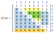
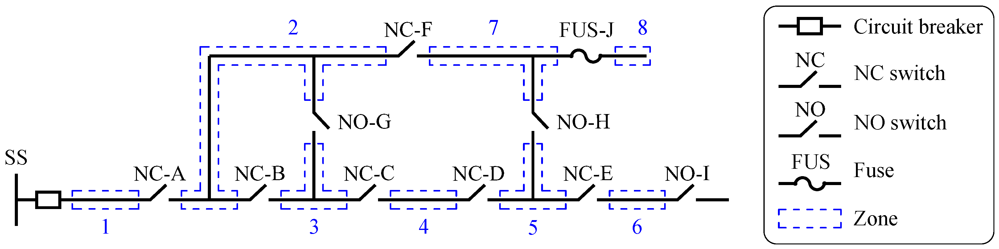
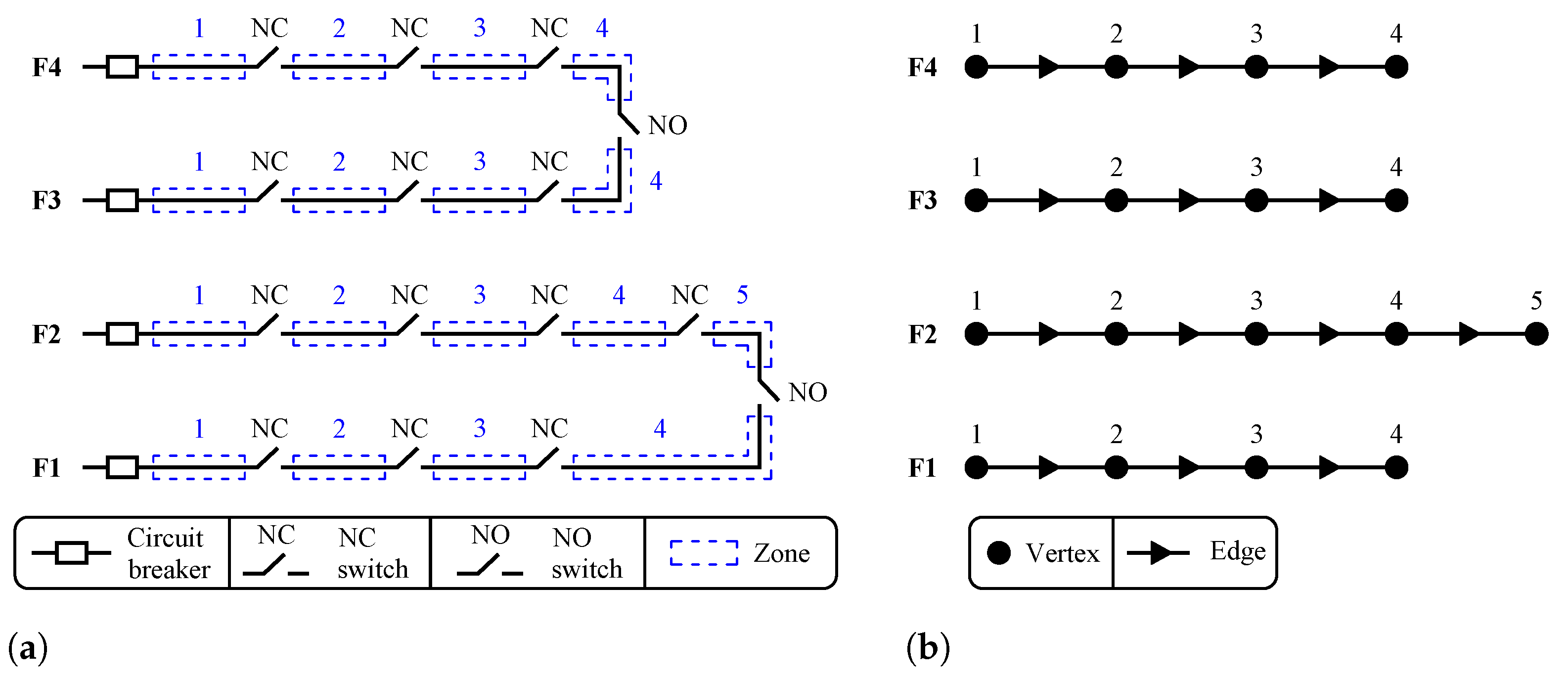
The analytical assessment of reliability is based on the classification of the zones regarding their capacity for restoration after a permanent fault in the distribution feeder. In this way, when a fault occurs in a given zone, the zones of the feeder are subsequently classified as follows.
  • Unaffected Zone (N): when the fault of a given zone does not interrupt the analyzed zone;
  • Recoverable Zone (R): when the fault of a zone interrupts the analyzed zone, but it is still possible to restore its supply through switching and re-connections within the same feeder;
  • Unrecoverable Zone (I): when the fault of a zone interrupts the analyzed zone with no possible restoration until the fault is fixed;
  • Transferable Zone (T): when the fault of a given zone interrupts the supply of the analyzed zone, but it remains possible to restore its supply by transferring the load to another feeder.
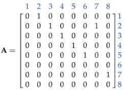
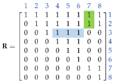
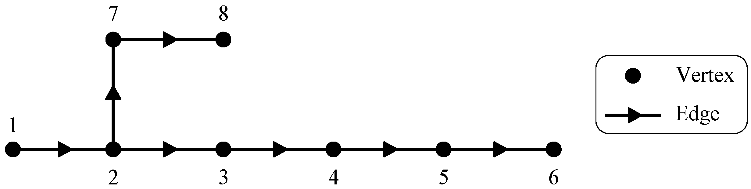
Now, using the matrix R and the classification described above, a matrix of classification can be defined, which will be termed Zone Classification Matrix (ZCM) and whose lines and columns of ZCM represent the zones of the feeder (Note that the lines represent the zones with fault). The matrix ZCM corresponding to the example feeder is given by (3). According to (3), the interruption of zone 7 interrupts all remaining zones of the feeders. However, the supply of zones 1 to 6 are restored by opening a sectionalizing device located upstream of zone 7.
Energies 15 05073 i003
From the matrix ZCM, it is also possible to obtain additional matrices with a similar structure which can be used to calculate reliability indices too, as proposed by [28]. These additional matrices are called Interruptions Quantity Matrix (IQM), Consumers Weighted Interruptions Quantity Matrix (CWIQM), Interruptions Duration Matrix (IDM), Consumers Weighted Interruptions Duration Matrix (CWIDM), and Consumption Weighted Interruption Matrix (CWIM).
To obtain the interruption frequency indices, first, the matrix IQM, which indicates the probability of permanent faults, is built according to the classification of the zones of the feeder contained in the matrix ZCM. Those zones classified as N are null in the matrix IQM, as the supply is not interrupted in these zones. In contrast, the failure rate (failures per year) of the zone under fault ( λ i ) is assigned to those zones classified as R, T, or I.
In addition, through the matrix IQM, it is possible to obtain the index CIF of the consumers in each zone j ( C I F j ), expressed in interruptions per year. The index CIF is defined as the sum of the elements of each column of the matrix IQM as:
C I F j = i = 1 n I Q M ( i , j ) = i = 1 n λ i
Each element of CWIQM contains the number of customers affected by interruptions in a year. The matrix CWIQM is obtained by multiplying IQM, element by element, with the respective number of consumers in the zone j ( N j ). The calculated SAIFI ( S A I F I c ), in interruptions per year, is obtained as the quotient of the sum of all elements of CWIQM and the total number of consumers (TC) according to:
S A I F I c = i = 1 n j = 1 n C W I Q M ( i , j ) T C = i = 1 n j = 1 n λ i N j T C
In contrast, the contribution of faults in zone i to the S A I F I c ( c S A I F I i ), in interruptions per year, is determined by the quotient of the sum of the elements of each line of CWIQM and TC:
c S A I F I i = j = 1 n C W I Q M ( i , j ) T C = j = 1 n λ i N j T C
The interruption duration indices are calculated based on the average restoration time ( t r e s ), and on the following parameters: (i) average fault location time ( t l ), (ii) average manual switching time ( t s w ) and (iii) average time to repair ( t r ), all expressed in hours. Additionally, the percentage of t l h in relation to t R h ( p l ) is included in the reliability assessment as follows:
p l = t l h t R h
Through the parameter p l , it is possible to insert t l into the reliability assessment, which is based on historical data of the occurrences of interruptions. In general, an urban feeder has a lower average time to locate a fault than a rural feeder. Therefore, to consider this fact, t l , in hours, is calculated as a proportion p l of t r e s as:
t l = t r e s p l
The time t s w as well as t r , expressed in hours, are determined using the repair time in percentage ( p r ) of the difference between t r e s and t l :
t s w = ( t r e s t l ) ( 1 p r ) and
t r = ( t r e s t l ) p r ,
with p r being empirically assumed as p r = 70 %, due to the unavailability of data related to switching and repair time in the historical data of occurrences of interruptions.
The average restoration time of each zone depends on their classification in the matrix ZCM and on the protection or switching situation (A, B or C), as indicated in Table 1.
The situation A (Table 1) refers only to the blowing of a fuse. Therefore, the restoration times apply only to those zones classified as N and I. In this case, the restoration time of a zone classified as N is null, and the restoration time of zone I is given by the sum of t l and t r , as shown in Table 1.
The situation B refers to the opening of the nearest NC switch upstream of the faulted zone. Therefore, the restoration times apply only to zones classified as R and I. In this case, the restoration time of zone R is given by the sum of t l and t s w . On the other hand, the restoration time of zone I is given by the sum of t l , t s w and t r .
Finally, the situation C refers to (i) the opening of the nearest NC switch upstream of the faulted zone, (ii) an additional NC switch that isolates the fault, and (iii) a NO switch. Therefore, the restoration times apply to zones R, T, and I. In this case, the restoration time of zones R and T is given as the sum of t l and 2 t s w . On the other hand, the restoration time of zone I is obtained from the sum of t l , 2 t s w , and t r .
In the matrix ZCM of the example feeder given by (3), situation A occurs with zone 8 under fault, while situation B with zones 6 or 7 under fault, and situation C for zones 2, 3, 4 or 5. In case of a fault in zone 1, it is not possible to restore the supply to any zone before the fault is repaired.
The Interruption Duration Matrix (IDM), expressed in hours per year, is determined through the product between the restoration time of each zone and the failure rate of the failed zone ( λ i ). The value of the CID, in hours per year, of the consumers in each zone j ( C I D j ) is determined by the sum of each column of the matrix IDM as follows:
C I D j = i = 1 n I D M ( i , j ) = i = 1 n λ i t r e s ( i , j )
Now, the matrix CWIDM is obtained by multiplying the matrix IDM element by element with the respective number of consumers in the zone j ( N j ). On the other hand, the calculated SAIDI ( S A I D I c ), in hours per year, is obtained by the quotient of the sum of all elements of the matrix CWIDM and the corresponding TC:
S A I D I c = i = 1 n j = 1 n C W I D M ( i , j ) T C = i = 1 n j = 1 n λ i t r e s ( i , j ) N j T C
The contribution of faults in zone i to the S A I D I c ( c S A I D I i ), in hours per year, is determined by the quotient of the sum of the elements of each line of the matrix CWIDM and TC:
c S A I D I i = j = 1 n C W I D M ( i , j ) T C = j = 1 n λ i t r e s ( i , j ) N j T C
From the preceding expressions, the calculated ASAI ( A S A I c ), in pu, can be obtained using the S A I D I c :
A S A I c = 1 S A I D I c 8760
The index EENS can be determined using the matrix CWIM. In turn, this matrix is determined by multiplying the matrix IDM element by element with the respective average annual consumption of the zone j, named C j and expressed in MWh. Then, the calculated index EENS ( E E N S c ), in MWh per year, is obtained as the sum of all elements of CWIM as:
E E N S c = i = 1 n j = 1 n C W I M ( i , j ) 8760 = i = 1 n j = 1 n λ i t r e s ( i , j ) C j 8760
The contribution of faults in zone i to the index E E N S c ( c E E N S i ), in MWh per year, is defined as the sum of the elements of each line of CWIM as follows:
c E E N S i = j = 1 n C W I M ( i , j ) 8760 = j = 1 n λ i t r e s ( i , j ) C j 8760
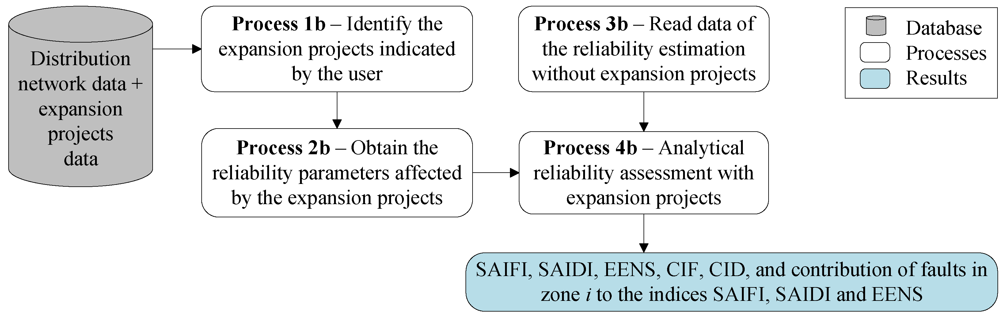
Finally, the expressions introduced and discussed in this section are used to estimate the reliability both with and without considering the execution of expansion projects. When no expansion projects are considered, the reliability indices correspond to the historical indices, as detailed in Section 3.1. In contrast, when expansion projects are considered, the indices reflect the impact of such projects on the reliability of the primary network, as described in Section 3.2.

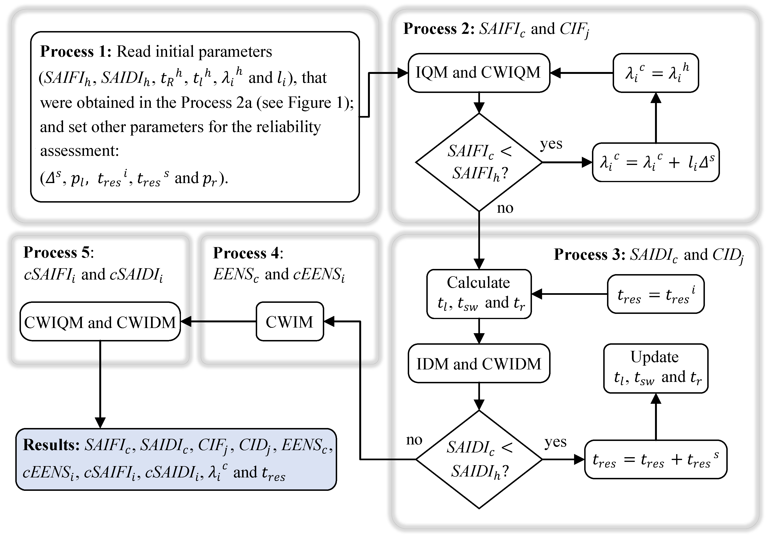
3.1. Adjustment of Estimated Reliability Indices to Historical Indices

To estimate the reliability without expansion projects, the initial failure rate per zone is calculated based on the historical interruptions. However, the database of the power distribution utility has data concerning the location of only part of the faults. Therefore, this information is assumed as unavailable. Consequently, the failure rate per zone is adjusted to the historical SAIFI ( S A I F I h ) after determining its initial value. Note also that inserting a failure rate per zone based on actual data of interruptions will incorporate a geographic link to the origin of the fault [17]. In addition, the failure rates per zone have different origins, such as winds, lightning, trees or vegetation, animals, material or equipment failure, etc. Thus, for example, the failure rates of zones containing vegetation must consider the presence of this vegetation as a possible cause of failure. Therefore, even with the uncertainties of the input data, the characteristics of the land/environment are weighted with the segmentation of failure rates per zone.
We developed a procedure similar to that used to estimate the failure rate to estimate the restoration time, which is also adjusted to the historical SAIDI ( S A I D I h ). However, the initial restoration time is assigned before the algorithm begins, and is further not based on the history of interruptions.
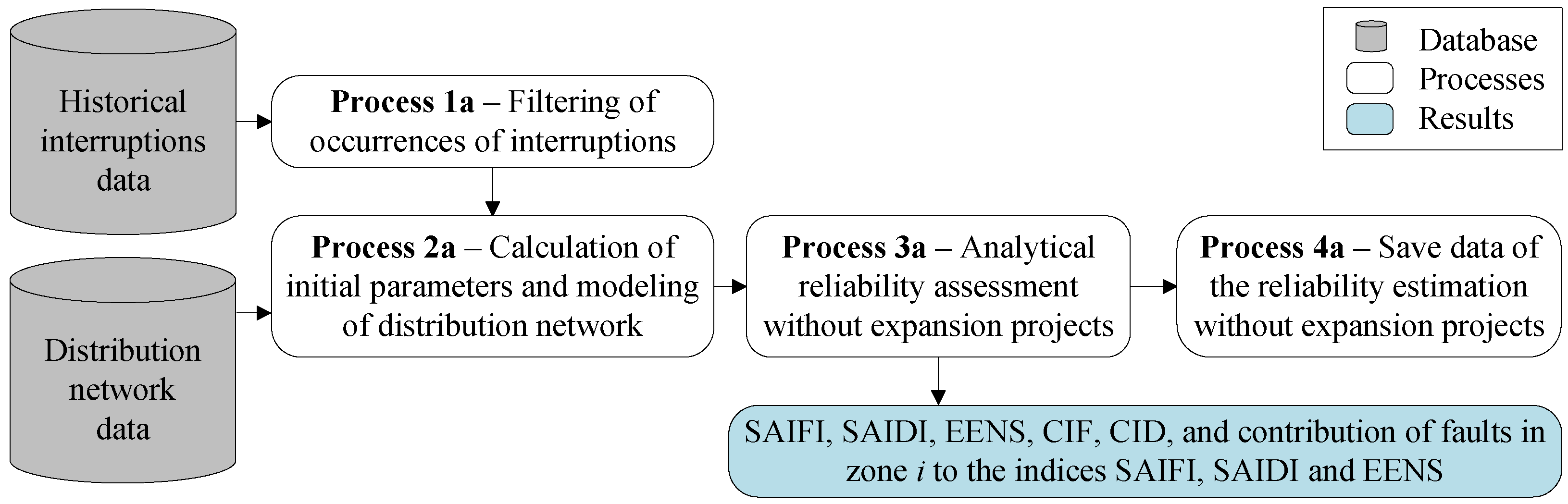
The flowchart in Figure 5 illustrates all the procedures we developed to adjust the estimated indices of reliability to their historical values.
In Process 1 (Figure 5), the initial data obtained in Process 2a (Figure 1) are read ( S A I F I h , S A I D I h , t R h , t l h , λ i h and l i ). In addition, values are assigned to the following parameters: (i) failure rate step per length ( Δ s ), in failure / km · year ; (ii) parameter p l ; (iii) initial restoration time ( t r e s i ), in hours; (iv) step for t r e s ( t r e s s ), in hours; and (v) parameter p r .
In Process 2, the algorithm first calculates the indices concerning the interruption frequency. This is an iterative process, in which the calculated failure rates per zone i ( λ i c ) (failures per year) start with the values of λ i h ; then, after each iteration, a failure rate of l i Δ s in failures per year is added to λ i c , until S A I F I c is adjusted to S A I F I h . Finally, the indices C I F j are generated through the matrix IQM.
Process 3 is dedicated to the estimation of indices related to the interruption duration. In this iterative process, t r e s starts with the value of t r e s i , and then t l , t s w and t r are calculated. At each iteration, t r e s s is added to t r e s ; subsequently, t l , t s w and t r are updated. The process stops when S A I D I c equals S A I D I h , after which the indices C I D j are obtained from the matrix IDM.
The indices E E N S c and c E E N S i are calculated in Process 4 using the matrix CWIM. Finally, in Process 5, the indices c S A I F I i and c S A I D I i are calculated through the matrices CWIQM and CWIDM, respectively.

3.2. Assessment of the Impact of Expansion Projects on the Reliability of the Primary Network

Planning the expansion of power distribution systems takes into account the addition, replacement or reinforcement of different types of devices, distribution lines, or substations [21,22]. Some of the alternatives for expansion projects aiming to improve the reliability of the network are (i) the division of primary feeders; (ii) installation of switches with interconnection with an adjacent feeder; (iii) the installation of circuit breakers, sectionalizing switches, reclosers, or fuses; (iv) automation of sectionalizing switches; (v) installation of fault indicators; and (vi) the reconductoring of the primary network by covered conductors. Furthermore, the reliability of active distribution networks can be improved through additional alternatives, such as islanded operation through post-fault reconfiguration and energy supply through distributed generation, energy storage systems, and electric vehicle charging stations. These alternatives can help reduce the duration of interruptions and thus improve reliability indices [7].
Although the proposed framework allows the incorporation of different types of expansion projects, this article will illustrate the impact of those alternatives of expansion that most affect reliability, namely (i) installation of an NC sectionalizing switch, (ii) installation of an NO switch with interconnection to an adjacent feeder, (iii) automation of NC sectionalizing switches, and (iv) reconductoring of medium-voltage (MV) feeders.
A distribution network can be segmented using sectionalizing devices, which allow fault isolation during contingency situations [31]. Furthermore, installing a NC sectionalizing switch in one zone creates two new zones. Thus, installing a NC switch in a given zone x generates the new zones x 1 and x 2 , and hence the number of consumers in x 1 and x 2 must be recalculated. Further, the failure rate of zone x ( λ x ), the length of x ( l x ), the length of x 1 ( l x 1 ) and the length of x 2 ( l x 2 ) are then required to determine the failure rates of the new zones, λ x 1 and λ x 2 .
λ x 1 = λ x l x l x 1 and λ x 2 = λ x l x l x 2 .
NO switches between adjacent feeders enable load transfer between feeders, while NO switches with vertices belonging to the same feeder enable restoration within the feeder [32]. Thus, using this reconfiguration makes it possible to reduce the duration of interruptions. According to the proposed framework, installing a NO switch requires updating the switches N O s and N O e by including the respective vertices at which they are installed.
Within the context of the automation of distribution systems, the outage management system (OMS) performs fault location and isolation, and the restoration of energy supply, thus helping to reduce the duration of interruptions and, therefore, improving the quality of services [33]. Besides, the automation of NC sectionalizing switches reduces t s w due to the remote-controlled operation. In addition, t l can be reduced if the fault location can be made easier when switches with an automated protection functionality are used [34]. To illustrate the reliability improvement provide by the automation of sectionalizing switches, the author of [28] reported that in some cases t s w can be reduced to zero and t l reduced in 70 % for faults that occur in the first zone downstream of the automated switch [28].
The reconductoring of MV feeders is an alternative to expansion plans aiming to improve reliability, since conductors with lower failure rates can be installed. The adoption of covered conductors in overhead distribution lines leads to reduced failure rates compared with bare conductors [35]. Covered conductors have the advantage of reduced short-circuit currents when distribution lines come into contact, for example, with vegetation. To estimate and illustrate the impact of reconductoring, we adopted a reduction in the λ i c for the zone i whose conductors have been replaced, similar to what was assumed in [28].

4. Validation and Application Examples

In this section, we discuss the validation of the proposed method using the Roy Billinton Test System (RBTS) [29]. Further, we implemented the algorithm shown in the flowchart of Figure 1 without considering a failure rate per zone based on the historical faults in each zone. This implementation was called correlated method and will serve the purpose of comparison with the proposed method. Finally, the algorithms corresponding to both methods were implemented in Matlab® [36].

4.1. Roy Billinton Test System

The RBTS consists of 5 load buses (bus2 – bus6) with different characteristics [29]. The distribution network at bus 5 of the RBTS is composed of typical urban loads, such as residences, offices, and commercial buildings, among others. This network also consists of four 11 kV feeders (F1–F4), 43 sections, and 26 load-points (LP), as illustrated in Figure 6. In addition, this network has 8 circuit breakers, 13 NC sectionalizing switches, and 2 NO switches. The number and the type of consumers, the average and peak loads at each LP, along with the length of each section of the network are available in [29]. Thus, due to the characteristics described, we chose the distribution network at bus 5 of the RBTS to test and validate the proposed method. Additional data and results for this case study are available in Supplementary Materials.
The zone diagram of the distribution network at bus 5 of the RBTS was obtained from the distribution network in Figure 6, as illustrated in Figure 7a. The feeders F1, F3, and F4 have 4 zones and 3 NC sectionalizing switches, while the feeder F2 has 5 zones and 4 NC sectionalizing switches. The oriented graph representing the distribution network at bus 5 of the RBTS is illustrated in Figure 7b.
Given that no historical data are available for RBTS, for our case study, the implemented algorithm assigns historical values for reliability indices, fault location and repair times, and failure rates for each zone. Thus, the indices given in [29] were considered as the historical values of the RBTS. Hence, 0.2325 interruptions/year and 3.5512 h/year were assigned to S A I F I h and S A I D I h , respectively. Additionally, due to the lack of historical data on fault location and restoration times for the RBTS, the parameters t l h and t R h could not be estimated. Therefore, we assigned approximately 60 % to p l . Besides, the historical failure rates shown in Table 2 were used. In addition, the following parameters were adopted in the implemented algorithm: Δ s = 10 6 failure/km.year, t r e s i = 17 h, t r e s s = 10 4 h and p r = 70 %.

4.1.1. Reliability Estimation without Expansion Projects

The reliability indices estimated without expansion projects resulted in 0.2325 interruptions/year for S A I F I c and 3.5512 h/year for S A I D I c . For comparison, together with those indices obtained through the correlated and proposed methods, Table 3 also contains the reliability indices obtained in [29]. Thus, according to Table 3, the S A I F I c and S A I D I c obtained with both methods we propose here correspond to those presented in [29], as expected. This similarity is because the algorithm adjusts S A I F I c and S A I D I c to the values assigned to S A I F I h and S A I D I h , which proves that both methods (correlated and proposed) converge to the same values. As a further consequence, the A S A I c values obtained by the correlated and the proposed methods are the same as those reported by [29].
As can be observed in Table 3, the values of E E N S c obtained with the correlated and proposed methods are slightly different from that given in [29]. This difference arises because, when reliability indices are estimated, both algorithms adjust the failure rate of each zone and repair times based on S A I F I h and S A I D I h . In contrast, in [29], failure rates and repair times per load node are calculated based on failure rates and repair times for individual components such as transformers, circuit breakers, buses, and lines [37]. The way that each method determines failure rates and repair times change those indices that are assessed for each load node (CIF and CID). Consequently, the estimated values for the E E N S c are also different for each method.
Concerning the interruption times, we obtained t r e s = 17.93 h, t l = 10.76 h, t s w = 2.15 h, and t r = 5.02 h. The failure rates per zone, in failures per year, obtained through the proposed method can be seen in Table 4, according to which zones 3, 4, and 5 of feeder F2 (in bold) have the highest failure rates compared to the rates of the remaining zones. Note also that these zones coincide with the zones that have the highest historical failure rates, highlighted in bold in Table 2.
The failure rates per zone in failures per year obtained through the correlated method are given in Table 5. Compared with the failures of other zones, the failure rates of zone 1 of feeder F1 and those of zone 4 of feeder F4 are the highest, which can be in part explained by the fact that these zones are 2.1 km long and, therefore, are the longest, as also indicated in [29].
The results in Table 4 and Table 5 also highlight that each method indicates a different zone with highest failure rates. This is because the proposed method considers the historical faults of each zone and, subsequently, distributes the failure rates according to the length of each zone. On the other hand, the correlated method only distributes the failure rates according to the length of each zone.
Table 6 reproduces the contribution of faults in each zone to the indices S A I F I c , S A I D I c , and E E N S c obtained through the proposed method. The values in bold indicate the zones in which the faults most contribute to S A I F I c and S A I D I c (zone 5 of feeder F2), as well as the zone in which the faults most contribute to E E N S c (zone 2 of feeder F1).
The contribution of faults in each zone to the indices S A I F I c , S A I D I c , and E E N S c obtained through the correlated method are presented in Table 7. The values in bold refer to zones that most contributes to S A I F I c (zone 1 of feeder F1), S A I D I c (zone 1 and 2 of feeder F1), and E E N S c (zone 2 of feeder F1).
A comparison between the values in bold in Table 6 and Table 7 reveals that concerning the highest contributions to S A I F I c and S A I D I c , each method indicates a different zone, as the proposed method indicates zone 5 of feeder F2 whereas the correlated method, zones 1 and 2 of feeder F1.
From the results discussed above, the contribution of faults in zones to reliability indices can help planners to find out and decide which expansion project is more advantageous in terms of reliability improvement. The comparison above also stresses the relevance of the fault history to the estimation of reliability, as it can directly affect the choice of the zone to execute a given expansion project, thus highlighting an advantage of the proposed method over the correlated method.
The reliability indices calculated assuming that no expansion projects are executed help estimate the impact of expansion alternatives on reliability, as these indices are used for sensitivity analysis of parameters related to the zones affected by expansion projects. Thus, the data required to estimate reliability indices without projects are stored and used later to assess the impact of expansion projects on reliability.

4.1.2. Estimation of Reliability Considering Expansion Projects

The prioritization of the execution of expansion alternatives takes into account the reliability indices estimated without projects. Note that expansion projects are indicated by the user of the framework; further, the results of the estimation without projects help the designer to select the best expansion alternatives among those possible. Besides, the contribution of faults within zones to S A I F I c is used afterward to guide the reconductoring of primary network zones with covered conductors. On the other hand, the faults contributions of zones to S A I D I c are used to guide the automation of sectionalizing switches.
Initially, we illustrate the replacement of conductors with covered conductors inside zone 5 of feeder F2, given that the fault contribution to S A I F I c of this zone is the highest of the distribution network (Table 6). The execution of this expansion project reduces the failure rate for this zone from 0.0853 to 0.0427 failure/year, which is due to the assumed reduction of 50% in the failure rate of the reconductored zone. As a result, the contribution of faults in zone 5 of feeder F2 to S A I F I c reduced from 0.0233 to 0.0117 interruptions/year, the contribution to S A I D I c reduced from 0.3305 to 0.1652 h/year, while the contribution to E E N S c reduced from 2.8182 to 1.4091 MWh/year. Furthermore, other reliability indices also changed, as shown in Table 8. The S A I F I c reduced by 5.03 % , while S A I D I c by 4.65 % , and E E N S c by 3.66 % ; in contrast, the A S A I c increased.
Given that the feeder has a circuit breaker at the beginning, the proposed reconductoring impacted only those reliability indices evaluated by load nodes of feeder F2 (CIF and CID). Thus, the index CIF decreased from 0.2990 to 0.2563 interruptions/year and the index CID of all zones of feeder F2 also decreased. The index CID of zone 5 of feeder F2, which was the highest for the distribution network for the case without expansion projects, decreased from 4.6683 to 3.9040 h/year. Note also that this expansion project will not affect the CIF or CID of the other zones if a fuse upstream of a reconductored zone is assumed, due to the characteristic of this device. In the event of a fault in this zone, the other zones will then be classified as N in the matrix ZCM.
In what follows, we illustrate the automation of NC sectionalizing switches for the switch upstream of zone 5 of feeder F2, as this zone has the highest fault contribution to S A I D I c without expansion projects. The automation of this switch reduced the contribution of faults in zone 5 of feeder F2 to S A I D I c from 0.3305 to 0.1046 h/year and the contribution to E E N S c from 2.8182 to 0.9292 MWh/year. As a result, the interruption duration indices and E E N S c were also impacted, as shown in Table 9. The S A I D I c decreased 6.36 % and E E N S c 4.91 % , whereas A S A I c increased. In contrast, the S A I F I c remained unchanged, as the automation of sectionalizing switches does not change the frequency of interruptions.
Concerning the indices evaluated by load node, the index CIF of the zones was not affected by the automation of the sectionalizing switches, as expected. However, considering the proposed expansion project, the index CID for the zones of feeder F2 decreased. The index CID of zone 5 of feeder F2, which has the highest value without expansion projects, decreased from 4.6683 to 3.8429 h/year.

5. Application Examples—Real Distribution System

We used a distribution feeder located in Southern Brazil to validate the proposed method using initial failure rates by zone and the available historical data of interruptions. This feeder consists of a primary network operating at a MV of 23 kV and having overhead conductors with a total length of 49.86 km. Besides, we considered that the feeder has 10,947 customers connected at low voltage. Figure 8 shows the zone diagram of the feeder, which is composed of 60 zones and the following devices: 36 fuses, 23 manual NC sectionalizing switches, 6 manual NO switches connected to the same feeder, and a point to install a NO switch with interconnection to an adjacent feeder. Additional data and results for this case study are available in Supplementary Materials.

5.1. Estimation of Reliability without Expansion Projects

Initially, as described in Section 2.2, the data received from the power utility and referring to the feeder were processed in order to generate a database. Then, based on the data of interruptions for a three-year period, the historical reliability indices were calculated, and obtained 19.66 interruptions/year for S A I F I h and 10.86 h/year for S A I D I h . Analogously, we obtained t R h = 2.86 h and t l h = 1.97 h, thus leading to p l = 70 %. In addition, the algorithm assumed Δ s = 10 7 failure/km.year, t r e s s = 10 4 h, t r e s i = 0.3 h, and p r = 70 %.
Table 10 shows reliability indices obtained through the correlated and proposed methods. According to this table, due to the adjustment of these indices to the values of S A I F I h and S A I D I h , respectively, the S A I F I c and S A I D I c obtained by both methods converged to the same value. As a further consequence, the A S A I c for both methods is the same too. The difference between S A I F I c and S A I F I h is related to the parameter Δ s adopted, while the difference between S A I D I c and S A I D I h to the parameter t r e s s adopted. Increasing these parameters can reduce the computational load required for the simulation, but simultaneously reduce the accuracy of the estimations. From Table 10, a good agreement between the values obtained for the E E N S c can be recognized.
Using the proposed and the correlated method, we obtained t r e s = 0.63 h, t l = 0.44 h, t r = 0.13 h and t s w = 0.06 h for the times related to interruptions. Additionally, failure rates per zone, in failures per year, were also determined using both methods, with the corresponding values being available as Supplementary Material.
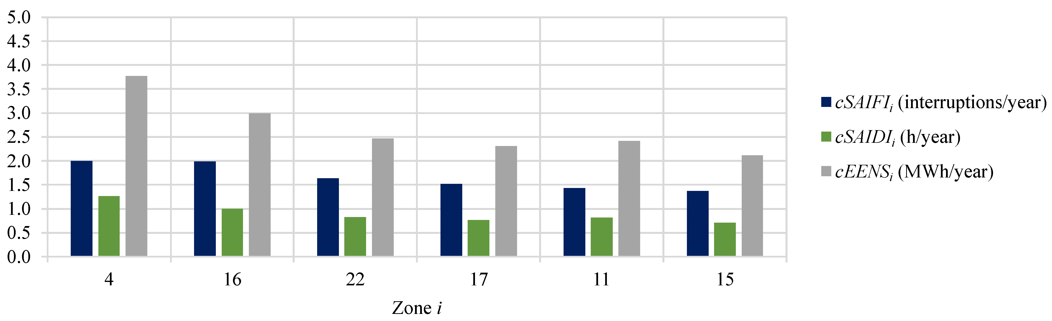
The six zones in which faults most contribute to the indices S A I F I c , S A I D I c , and E E N S c are highlighted in orange in Figure 8. Additionally, the highest contributions of faults in these zones to the indices S A I F I c , S A I D I c , and E E N S c are shown in Figure 9. Faults in zone 4 contribute most to the indices S A I F I c , S A I D I c , and E E N S c ; faults in zone 4 account for approximately 10% of S A I F I c , and 12% of S A I D I c and E E N S c .
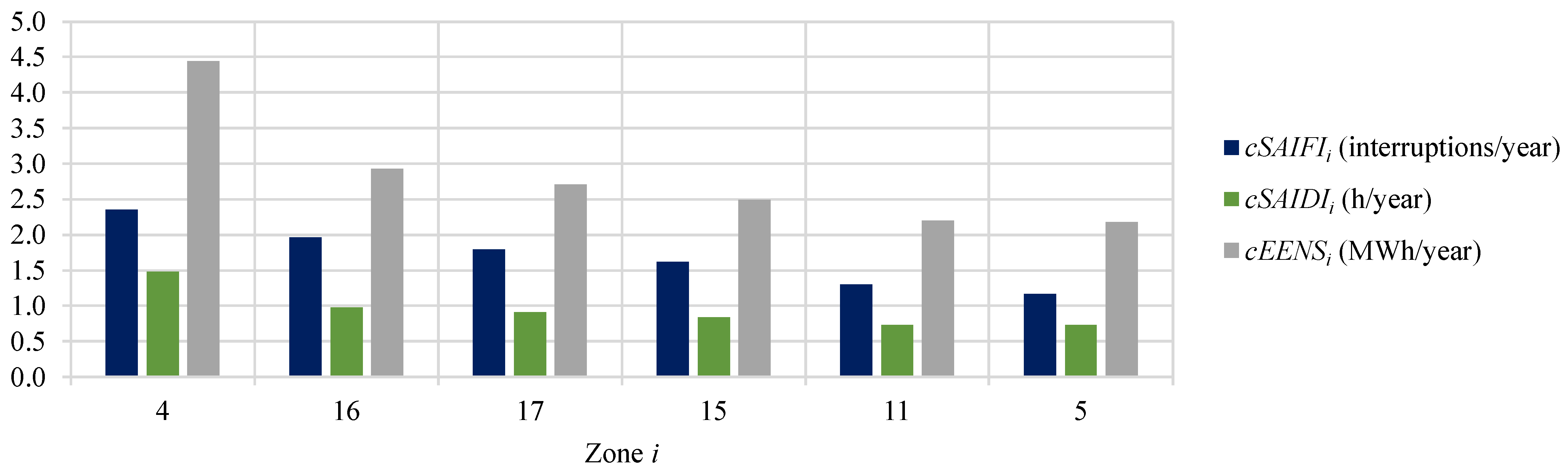
Figure 10 confirms that each method (correlated and proposed) indicates a different zone with the highest fault contribution to the indices S A I F I c , S A I D I c , and E E N S c . The correlated method estimates failure rates proportionally to the length of the zones and without considering the history of interruptions. As a consequence, the zones with the highest values of fault contribution to the S A I F I c correspond to the longest which, in addition, are not protected by a fuse, namely zone 4 (4.06 km), 16 (3.37 km), 17 (3.09 km), 15 (2.79 km), and 11 (2.24 km).
The zones with the highest indices CIF and CID estimated with the proposed method are highlighted in blue in Figure 8. The five highest values for the index CIF refer to zones 41, 33, 39, 56, and 46, respectively with 23.38 , 22.41 , 22.17 , 22.10 , and 21.63 interruptions/year. On the other hand, the zones with the highest values for the index CID are zones 41, 56, 39, 33, and 49 having, respectively, 13.12 , 12.35 , 12.22 , 12.21 , and 11.98 h/year.
The fault contribution of each zone to the indices S A I F I c , S A I D I c , and E E N S c were obtained through the proposed algorithm. The values of these indices will be used as a basis to prioritize (i) the sectionalizing switches to be automated and (ii) the existing network zones to be replaced by conductors with lower failure rates in connection with a reconductoring plan.

5.2. Estimation of Reliability Considering Expansion Projects

Initially, this study assumes that a manual type NC sectionalizing switch was installed within zone 11 of the feeder, since, among the zones with upstream NC sectionalizing switches, this zone contributes significantly to S A I D I c . Zone 11 of this feeder is part of the primary network and 2.24 km long, which corresponds to 4.5% of the total length of the primary network. In addition, this zone has 654 customers and a failure rate of 1.43 failure/year.
The switch installed in zone 11, between sectionalizing switches 0513 and 0191, divides this zone into two parts, named 11a and 11b and having, respectively, 251 and 403 customers. Further, zones 11a and 11b are, respectively, 0.56 and 1.67 km long within the primary network; they exhibit failure rates of 0.36 and 1.07 failure/year, respectively. Due to the installation of the sectionalizing switch, the index CID for zone 11a becomes 10.17 h/year, while that for zone 11b is 10.26 h/year. Thus, the indices CID of zones 11a and 11b are lower than the CID of zone 11, whose value is 10.31 h/year.
On the other hand, the indices S A I D I c and E E N S c remained almost unchanged after the installation of the NC sectionalizing switch, as we obtained 10.86 h/year and 32.31 MWh/year, respectively, for these indices. Moreover, the frequency of interruptions is also unaffected by installation of NC sectionalizing switches. In this case, the installation of the sectionalizing switch only changed the switching conditions of customers in zones 11a and 11b, considering the occurrence of faults in these zones. Therefore, there was no impact on the restoration classification of other zones.
Adding the fault contributions of zones 11a and 11b to the S A I D I c results in 0.803 h/year, a value lower than that determined for the fault contribution of zone 11 to S A I D I c ( 0.808 h/year). Likewise, the sum of fault contributions from zones 11a and 11b to the index E E N S c is 2.40 MWh/year and therefore lower than the contribution of zone 11 to the index E E N S c ( 2.42 MWh/year).
It is noteworthy that the installation of only one sectionalizing switch did not significantly impact the reliability indices considered. However, defining the location of sectionalizing switches with priority to those zones with the highest fault contributions to the S A I D I c helps in the restoration process of the zones considered more critical in terms of fault contributions to the duration of interruptions. Furthermore, the user can divide the zones into several parts by installing more sectionalizing switches.
Next, we analyzed the installation of a NO switch with interconnection to an adjacent feeder inside zone 13 (see Figure 8). The installation of this switch led to the indices S A I D I c = 10.65 h/year and E E N S c = 31.69 MWh/year, which represents a reduction of, respectively, 0.21 h/year and 0.62 MWh/year. Note also that under fault contingencies, more zones can be transferred to another feeder, thus reducing the time to restore these zones. However, the index CID for some zones may be higher, as is the case of zones (2–4), where CID increased around 0.23 h/year. This increase can be explained by the manual operation of more switches, which increases the total time for switching and, consequently, the restoration time of these zones.
To evaluate the impact on reliability coming from the automation of NC sectionalizing switches, firstly, we automated the nearest upstream sectionalizing switch inside the zone with the highest value of fault contribution to the S A I D I c . Then, we did the same with the nearest sectionalizing switches upstream of the two zones with the highest contribution of faults to the S A I D I c and successively with up to eight zones with the highest contribution of faults to the S A I D I c . The results obtained through this procedure for S A I D I c and E E N S c are shown, respectively, in Figure 11a,b, according to which S A I D I c and E E N S c 
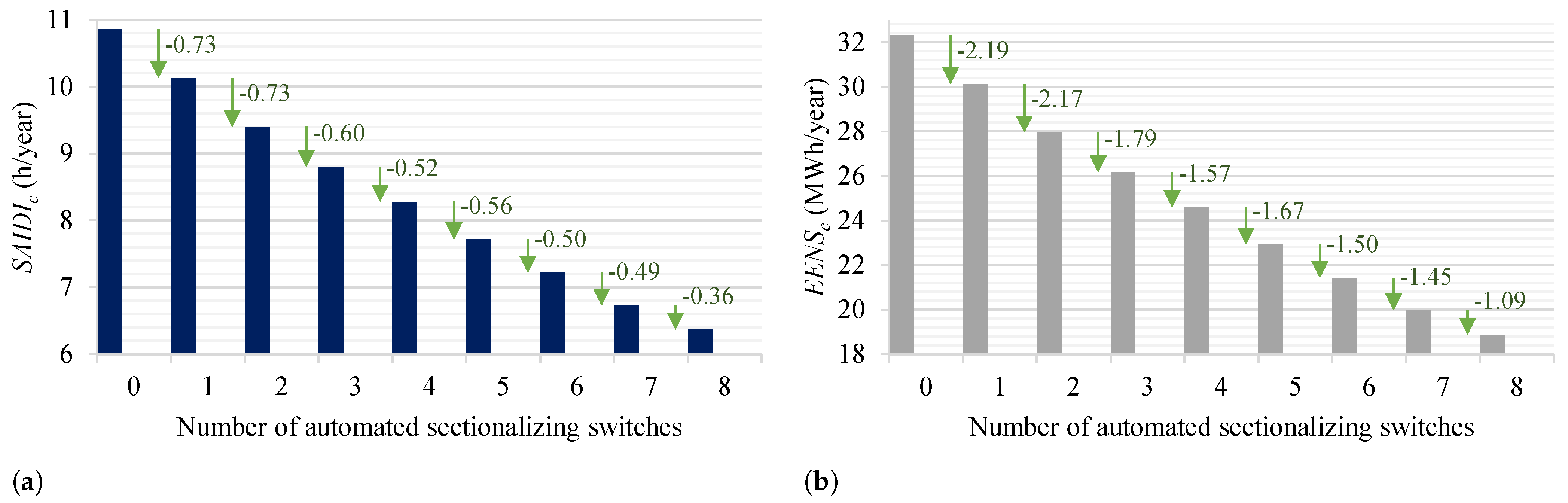
decrease when the number of automated switches increases. Additionally, note that without automation of switches, these indices represent the reliability without expansion projects. It is also worth noting that the S A I F I c is not affected by the automation of switches, as the energy supply cannot be restored in a time shorter than the minimum duration of sustained interruptions.
To assess the impact of reconductoring with covered conductors on S A I F I c , S A I D I c , and E E N S c , we consider here the reconductoring of zones of the network. Initially, zone 4 was reconductored, given that it has the highest contribution of faults to the S A I F I c . Then, the two zones with the highest fault contribution to the S A I F I c were reconductored, and so on, successively, up to ten zones with the highest values of fault contribution to the S A I F I c . Figure 12a,b, respectively, show S A I F I c and S A I D I c versus the number of reconductored zones. When no reconductoring occurs, no changes will take place in the network. When the reconductoring occurs inside zone 4, we obtain E E N S c = 30.43 MWh/year, which represents a reduction of 1.88 MWh/year, while with the reconductoring of eight zones, we obtain E E N S c = 22.32 MWh/year, thus a reduction of 9.99 MWh/year.
The case involving reconductoring illustrates the potential of the proposed method to mitigate the frequency of interruptions, which is intimately related to the consumer satisfaction with the services provided by power distribution utilities. The results thus far discussed also highlight the importance of considering, during planning stages, changes in the network that can lead to a reduction in failure rates.

6. Conclusions

In this article, we introduced a framework for inserting reliability into studies of planning the expansion of primary distribution networks. Further, we described how to determine matrices which allow estimating the most relevant reliability indices, such as SAIFI and SAIDI. The framework proposed and detailed here is illustrated in a flowchart, which describes an algorithm to analytically assess reliability. This algorithm also allows estimating reliability indices, which are adjusted to historical indices of the primary distribution network. We illustrated the potential use and advantages of the proposed framework through a case study using the distribution network at bus 5 of the RBTS and also using a real distribution feeder. The case study confirmed that applying the proposed framework, significant improvements can be achieved in reliability indices. Finally, the extent of these improvements depend on the particular expansion project considered.
The results we presented in this paper showed that the proposed framework can guide the location of the installation and automation of sectionalizing switches by identifying the zones in which the faults most contribute to the reliability indices. In addition, the numerical results demonstrated a positive impact on the reliability of a real feeder, which comes from the installation of an NC sectionalizing switch in the most critical zone of this feeder. Additionally, an improvement was also observed in the reliability of the real feeder as more sectionalizing switches are automated, and more network zones are reconductored with conductors with lower failure rates. Therefore, the proposed framework can support the decision of investments in network expansion projects during planning stages. The impact on reliability coming from different expansion projects can be measured and compared by the user of the proposed framework to achieve the required reliability indices.
Due to the flexibility of the proposed framework, future work may address the insertion of several other expansion projects that impact the reliability of power distribution systems, including distributed energy resources. The incorporation of the expansion of the network to meet load, usually called greenfield planning, is also an alternative for future study, since the proposed framework can be adjusted to adopt different failure rates. Finally, we are currently expanding the framework introduced in this article to consider the costs of investments in expansion projects indicated by the user.

Supplementary Materials

The following supporting information can be downloaded at: https://www.mdpi.com/article/10.3390/en15145073/s1.

Author Contributions

Conceptualization, G.L.A., G.A.d.C. and M.R.; methodology, G.L.A., G.A.d.C. and M.R.; validation, R.C.L.; investigation, G.L.A., G.A.d.C.; writing—original draft preparation, G.L.A., G.A.d.C. and M.R.; writing—review and editing, R.C.L., L.A.P.; supervision, M.R.; project administration, M.R.; funding acquisition, M.R., R.C.L., L.A.P. All authors have read and agreed to the published version of the manuscript.

Funding

This study was financed in part by the Coordenação de Aperfeiçoamento de Pessoal de Nível Superior—Brasil (CAPES)—Finance Code 001. This research was funded by Research and Development program of CEEE Grupo Equatorial Energia, regulated by ANEEL, project number PD-05707-2006/2020. Finally, the authors thank the National Council for Scientific and Technological Development (CNPq)—Brazil—for the financial support (grant number 306126/2019-2).

Institutional Review Board Statement

Not applicable.

Informed Consent Statement

Not applicable.

Data Availability Statement

The data and results for the case studies presented in this article are available in Supplementary Materials.

Conflicts of Interest

The authors declare no conflict of interest.

References

  1. Masoum, M.; Fuchs, E. Power Quality in Power Systems and Electrical Machines, 2nd ed.; Academic Press: Cambridge, MA, USA, 2015. [Google Scholar]
  2. Georgilakis, P.S.; Hatziargyriou, N.D. A review of power distribution planning in the modern power systems era: Models, methods and future research. Electr. Power Syst. Res. 2015, 121, 89–100. [Google Scholar] [CrossRef]
  3. Escalera, A.; Hayes, B.; Prodanović, M. A survey of reliability assessment techniques for modern distribution networks. Renew. Sustain. Energy Rev. 2018, 91, 344–357. [Google Scholar] [CrossRef]
  4. Alotaibi, I.; Abido, M.; Khalid, M.; Savkin, A. A comprehensive review of recent advances in smart grids: A sustainable future with renewable energy resources. Energies 2020, 13, 6269. [Google Scholar] [CrossRef]
  5. Chaves, T.; Martins, M.; Martins, K.; de Macedo, A.; de Francisci, S. Application study in the field of solutions for the monitoring distribution transformers of the overhead power grid. Energies 2021, 14, 6072. [Google Scholar] [CrossRef]
  6. Billinton, R.; Allan, R.N. Reliability Evaluation of Engineering Systems: Concepts and Techniques, 2nd ed.; Plenum Press: New York, NY, USA, 1992. [Google Scholar]
  7. Aschidamini, G.L.; da Cruz, G.A.; Resener, M.; Ramos, M.J.S.; Pereira, L.A.; Ferraz, B.P.; Haffner, S.; Pardalos, P.M. Expansion Planning of Power Distribution Systems Considering Reliability: A Comprehensive Review. Energies 2022, 15, 2275. [Google Scholar] [CrossRef]
  8. Billinton, R.; Allan, R.N. Reliability Evaluation of Power Systems, 2nd ed.; Plenum Press: New York, NY, USA, 1996. [Google Scholar]
  9. Lotero, R.; Contreras, J. Distribution system planning with reliability. IEEE Trans. Power Deliv. 2011, 26, 2552–2562. [Google Scholar] [CrossRef]
  10. IEEE. IEEE Std 1366-2012; IEEE Guide for Electric Power Distribution Reliability Indices. IEEE: Piscataway, NJ, USA, 2012; pp. 1–43.
  11. Escalera, A.; Castronuovo, E.; Prodanović, M.; Roldán-Pérez, J. Reliability assessment of distribution networks with optimal coordination of distributed generation, energy storage and demand management. Energies 2019, 12, 3202. [Google Scholar] [CrossRef] [Green Version]
  12. Chowdhury, A.; Koval, D. Power Distribution System Reliability: Practical Methods and Applications; Wiley: Hoboken, NJ, USA, 2009. [Google Scholar]
  13. Billinton, R.; Li, W. Reliability Assessment of Electric Power Systems Using Monte Carlo Methods, 1st ed.; Springer: New York, NY, USA, 1994. [Google Scholar]
  14. Brown, R. Electric Power Distribution Reliability, 2nd ed.; CRC Press: Boca Raton, FL, USA, 2008. [Google Scholar]
  15. López-Prado, J.; Vélez, J.; Garcia-Llinás, G. Reliability evaluation in distribution networks with microgrids: Review and classification of the literature. Energies 2020, 13, 6189. [Google Scholar] [CrossRef]
  16. Tabares, A.; Munoz-Delgado, G.; Franco, J.; Arroyo, J.; Contreras, J. An Enhanced Algebraic Approach for the Analytical Reliability Assessment of Distribution Systems. IEEE Trans. Power Syst. 2019, 34, 2870–2879. [Google Scholar] [CrossRef]
  17. Sperandio, M. Planejamento da Automação de Sistemas de Manobra em Redes de Distribuição. Ph.D. Thesis, Federal University of Santa Catarina, Florianópolis, Brazil, 2008. [Google Scholar]
  18. Wang, C.; Zhang, T.; Luo, F.; Li, P.; Yao, L. Fault incidence matrix based reliability evaluation method for complex distribution system. IEEE Trans. Power Syst. 2018, 33, 6736–6745. [Google Scholar] [CrossRef]
  19. Zhang, T.; Wang, C.; Luo, F.; Li, P.; Yao, L. Analytical Calculation Method of Reliability Sensitivity Indexes for Distribution Systems Based on Fault Incidence Matrix. J. Mod. Power Syst. Clean Energy 2020, 8, 325–333. [Google Scholar] [CrossRef]
  20. Li, R.; Wang, W.; Chen, Z.; Jiang, J.; Zhang, W. A review of optimal planning active distribution system: Models, methods, and future researches. Energies 2017, 10, 1715. [Google Scholar] [CrossRef] [Green Version]
  21. Georgilakis, P.; Arsoniadis, C.; Apostolopoulos, C.; Nikolaidis, V. Optimal allocation of protection and control devices in smart distribution systems: Models, methods, and future research. IET Smart Grid 2021, 4, 397–413. [Google Scholar] [CrossRef]
  22. Resener, M.; Haffner, S.; Pereira, L.; Pardalos, P. Optimization techniques applied to planning of electric power distribution systems: A bibliographic survey. Energy Syst. 2018, 9, 473–509. [Google Scholar] [CrossRef]
  23. Jooshaki, M.; Abbaspour, A.; Fotuhi-Firuzabad, M.; Muñoz-Delgado, G.; Contreras, J.; Lehtonen, M.; Arroyo, J.M. An Enhanced MILP Model for Multistage Reliability-Constrained Distribution Network Expansion Planning. IEEE Trans. Power Syst. 2022, 37, 118–131. [Google Scholar] [CrossRef]
  24. Tabares, A.; Muñoz-Delgado, G.; Franco, J.F.; Arroyo, J.M.; Contreras, J. Multistage reliability-based expansion planning of ac distribution networks using a mixed-integer linear programming model. Int. J. Electr. Power Energy Syst. 2022, 138, 107916. [Google Scholar] [CrossRef]
  25. Hamidan, M.A.; Borousan, F. Optimal planning of distributed generation and battery energy storage systems simultaneously in distribution networks for loss reduction and reliability improvement. J. Energy Storage 2022, 46, 103844. [Google Scholar] [CrossRef]
  26. Heidari, S.; Fotuhi-Firuzabad, M. Reliability evaluation in power distribution system planning studies. In Proceedings of the International Conference on Probabilistic Methods Applied to Power Systems (PMAPS), Beijing, China, 16–20 October 2016. [Google Scholar] [CrossRef]
  27. Heidari, S.; Fotuhi-Firuzabad, M.; Kazemi, S. Power Distribution Network Expansion Planning Considering Distribution Automation. IEEE Trans. Power Syst. 2015, 30, 1261–1269. [Google Scholar] [CrossRef]
  28. Dias, E.B. Avaliação de Indicadores de Continuidade e seu Impacto no Planejamento de Sistemas de Distribuição. Master’s Thesis, University of São Paulo, São Paulo, Brazil, 2002. [Google Scholar]
  29. Billinton, R. A test system for teaching overall power system reliability assessment. IEEE Trans. Power Syst. 1996, 11, 1670–1676. [Google Scholar] [CrossRef] [Green Version]
  30. Diestel, R. Graph Theory, 5th ed.; Graduate Texts in Mathematics; Springer: Berlin, Germany, 2017. [Google Scholar]
  31. Xie, K.; Zhou, J.; Billinton, R. Fast algorithm for the reliability evaluation of large-scale electrical distribution networks using the section technique. IET Gener. Transm. Distrib. 2008, 2, 701–707. [Google Scholar] [CrossRef]
  32. Zidan, A.; Khairalla, M.; Abdrabou, A.M.; Khalifa, T.; Shaban, K.; Abdrabou, A.; El Shatshat, R.; Gaouda, A.M. Fault Detection, Isolation, and Service Restoration in Distribution Systems: State-of-the-Art and Future Trends. IEEE Trans. Smart Grid 2017, 8, 2170–2185. [Google Scholar] [CrossRef]
  33. Zheng, H.; Cheng, Y.; Gou, B.; Frank, D.; Bern, A.; Muston, W. Impact of automatic switches on power distribution system reliability. Electr. Power Syst. Res. 2012, 83, 51–57. [Google Scholar] [CrossRef]
  34. Conti, S.; Rizzo, S.A.; El-Saadany, E.F.; Essam, M.; Atwa, Y.M. Reliability assessment of distribution systems considering telecontrolled switches and microgrids. IEEE Trans. Power Syst. 2014, 29, 598–607. [Google Scholar] [CrossRef]
  35. Li, M.B.; Su, C.T.; Shen, C.L. The impact of covered overhead conductors on distribution reliability and safety. Int. J. Electr. Power Energy Syst. 2010, 32, 281–289. [Google Scholar] [CrossRef]
  36. MATLAB, R2021a; The MathWorks Inc.: Natick, MA, USA, 2021.
  37. Allan, R.; Billinton, R.; Sjarief, I.; Goel, L.; So, K. A Reliability Test System For Educational Purposes - Basic Distribution System Data and Results. IEEE Trans. Power Syst. 1991, 6, 813–820. [Google Scholar] [CrossRef]
Figure 1. Flowchart of reliability assessment assuming no expansion of the distribution network.
Energies 15 05073 g001
Figure 2. Flowchart for the estimation of reliability considering expansion projects.
Energies 15 05073 g002
Figure 3. Feeder used as example to derive the model of the network.
Energies 15 05073 g003
Figure 4. Oriented graph of the example feeder.
Energies 15 05073 g004
Figure 5. Flowchart for the analytical assessment of reliability.
Energies 15 05073 g005
Figure 6. Distribution network at bus 5 of the RBTS [29].
Energies 15 05073 g006
Figure 7. Representation of the distribution network at bus 5 of the RBTS. (a) Zone diagram. (b) Oriented graph.
Energies 15 05073 g007
Figure 8. Zone diagram of the real distribution feeder used as example.
Energies 15 05073 g008
Figure 9. Zones with highest contribution of faults to the reliability indices obtained using the proposed method.
Energies 15 05073 g009
Figure 10. Zones with highest contribution of faults to the reliability indices obtained through the correlated method.
Energies 15 05073 g010
Figure 11. Impact of sectionalizing switches automation on reliability indices. (a) S A I D I c . (b) E E N S c .
Energies 15 05073 g011
Figure 12. Impact of reconductoring on reliability indices. (a) S A I F I c . (b) S A I D I c .
Energies 15 05073 g012
Table 1. Restoration time according to zone classification and protection or switching situation.
Zone ClassificationAverage Restoration Time  ( t res )
ABC
N0--
R- t l + t s w t l + t s w + t s w
T-- t l + t s w + t s w
I t l + t r t l + t s w + t r t l + t s w + t s w + t r
Table 2. Historical failure rates per zone.
Zone12345
λ i h
(failure/year)
F10.010.010.010.01
F20.010.010.040.040.04
F30.010.010.010.01
F40.010.010.010.01
Table 3. Reliability indices for the distribution network at bus 5 of the RBTS.
Ref. [29]Correlated MethodProposed Method
S A I F I c  (interruptions/year)0.23250.23250.2325
S A I D I c  (h/year)3.55123.55123.5512
A S A I c  (%)99.959599.959599.9595
E E N S c  (MWh/year)40.119439.669638.4903
Table 4. Failure rates per zone obtained through the proposed method.
Zone12345
λ i c
(failure/year)
F10.05870.05530.05180.0471
F20.03670.03670.07360.06670.0853
F30.04710.04830.04360.0553
F40.05530.05530.03670.0587
Table 5. Failure rate per zone obtained through the correlated method.
Zone12345
λ i c
(failure/year)
F10.06860.06370.05880.0523
F20.03760.03760.04740.03760.0637
F30.05230.05390.04740.0637
F40.06370.06370.03760.0686
Table 6. Contribution of faults in zones to the reliability indices obtained using the proposed method.
Zone12345
c S A I F I i
(int./year)
F10.01880.01770.01660.0151
F20.01000.01000.02020.01820.0233
F30.00450.00460.00420.0053
F40.01710.01710.01140.0182
c S A I D I i
(h/year)
F10.28660.29040.27210.1965
F20.12970.16380.32870.29770.3305
F30.05940.08990.06290.0697
F40.26190.25950.17230.2799
c E E N S i
(MWh/year)
F12.78893.07362.87992.1327
F21.19891.32372.65722.40612.8182
F31.68882.09611.85722.0849
F42.40142.81201.75212.5186
Table 7. Contribution of faults in zones to the reliability indices obtained using the correlated method.
Zone12345
c S A I F I i
(int./year)
F10.02200.02040.01890.0168
F20.01030.01030.01300.01030.0174
F30.00500.00510.00450.0061
F40.01980.01980.01160.0213
c S A I D I i
(h/year)
F10.33560.33560.30980.2184
F20.13310.16810.21200.16810.2476
F30.06600.10060.06840.0805
F40.30270.30000.17680.3278
c E E N S i
(MWh/year)
F13.26583.55263.27932.3712
F21.23081.35891.71341.35892.1111
F31.87772.34562.02052.4099
F42.77563.25031.79872.9493
Table 8. Impact of reconductoring on reliability indices.
Case without Expansion ProjectsCase with ReconductoringReduction (%)
S A I F I c  (int./year)0.23250.2208 5.03
S A I D I c  (h/year)3.55123.3860 4.65
A S A I c  (%)99.959599.9614
E E N S c  (MWh/year)38.490337.0812 3.66
Table 9. Impact of automation with switches on reliability indices.
Case without Expansion ProjectsCase with Switch AutomationReduction (%)
S A I F I c  (int./year)0.23250.23250
S A I D I c  (h/year)3.55123.3254 6.36
A S A I c  (%)99.959599.9620
E E N S c  (MWh/year)38.490336.6013 4.91
Table 10. Reliability indices obtained for a real distribution feeder.
Correlated MethodProposed Method
S A I F I c  (interruptions/year)19.6619.66
S A I D I c  (h/year)10.8610.86
A S A I c  (%)99.876099.8760
E E N S c  (MWh/year)32.3832.31
Publisher’s Note: MDPI stays neutral with regard to jurisdictional claims in published maps and institutional affiliations.

