Abstract
Methanol is considered to be a viable option for reducing greenhouse gas (GHG) emissions in shipping, the second-highest emitter after road freight. However, the use of fossil methanol is insufficient to meet climate change targets, while renewable methanol is yet unavailable on a commercial scale. This paper presents a novel biorefinery concept based on biomass solvolysis to produce crude lignin oil (CLO) from forest residues, a drop-in biofuel for methanol-propelled ships, and evaluates its environmental and economic profiles. In the base scenario, CLO can achieve emission saving of 84% GHG compared to fossil alternatives, and a minimum selling price (MSP) of $821 per ton of methanol equivalent (ME), i.e., within the range of the current bio-methanol production costs. The emission of GHGs of co-produced ethanol can be reduced by 67% compared to fossil analogues. The increase of renewable electricity share to 75% is capable of shrinking emissions by 1/5 vs. the base case, while fossil methanol losses, e.g., of that in cellulose pulp, can boost emissions by 63%. Low-pressure steam use in the biomass pretreatment, as well as biorefinery capacity increase by a factor of 2.5, have the greatest potential to reduce MSP of CLO to $530 and $614 per ton of ME, respectively.
1. Introduction
Maritime shipping plays an important role in trade and commerce, transporting more than 80% of all goods, and the demand for freight shipping is expected to grow further [1,2]. Although shipping is the least energy-intensive freight mode, it is the second-highest GHG emitter after road freight [3,4], mainly due to the use of much less refined fuels, such as heavy fuel oil (HFO) and marine diesel [2,4]. Overall, the shipping sector contributes 4 to 9% of the global sulphur oxides, 10 to 15% of nitrogen oxides and up to more than 2% of anthropogenic CO2 emissions, the latter expected to grow by 50% to 250% towards 2050 [2,5]. Other waterborne transport-related air pollutants posing additional risks to human health include particulate matter, non-methane volatile organic compounds and carbon monoxide [6].
The transition to biofuels is considered as a more promising short- to mid-term pathway towards climate-neutral shipping, though this mainly concerns drop-in fuel options, i.e., biofuels that can be blended with HFO and diesel [4]. However, these options are not yet available on a commercial scale [2,4], leaving aside fatty acid methyl ester (FAME) that, in fact, does not meet specifications required for many marine engines and has its own sustainability issues concerning its feedstock origin, and heavy vegetable oil (HVO), that is still a very costly option.
On the other hand, fossil methanol can be also regarded to as a short-term transitory solution for the shipping sector, with the potential to reduce its CO2 engine emissions by 20% compared to HFO [7], as well as to decrease sulphur oxides (SOx), nitrogen oxides (NOx) and particulate matter emissions by 99%, 60% and 95%, respectively [8]. Nonetheless, it is not enough to meet the decarbonization target set by the International Maritime Organization (IMO) aiming at the reduction of the total annual GHG emissions from international shipping by at least 50% vis-a-vis 2008 before 2050 [5]. Nowadays, there are over 20 methanol-propelled ships and more are coming, making viable a gradual transition to renewable methanol options [7]. At the same time, renewable methanol is not yet available on a commercial scale and features high production costs [9]. Moreover, the low energy density of methanol requires an up to three times more frequent bunkering compared to the current fossil fuels [2].
Lignocellulosic biofuels that can be blended with methanol, i.e., methanol drop-in fuels, offer a potential to improve the lifecycle emissions and calorific value of such blends, and, hence, can be also considered as a viable option for the short- to mid-term pathways to carbon-zero shipping.
While in the recent years the valorization of non-edible lignocellulosic carbohydrates to ethanol has attracted a large attention in the context of decarbonization of the road transport [10], lignin contained in biomass was mainly treated as a side stream and used for biorefinery internal energy supply [11]. In the meantime, biomass delignification using solvolysis technology offers an opportunity to valorize both streams. Recent studies showed the benefit of using methanol for the lignin-first upgrading of woody biomass with the production of cellulose pulp and lignin oil intermediate, where the latter comprises a mixture of lignin oligomers and C5 sugars in the methanol solvent able to target marine fuel application directly [12]. Later on, experimental trials at the multi-purpose pilot plant at the Chemelot Campus in Geleen, the Netherlands, were conducted to scale-up the solvolysis process up to 150 litres of crude lignin oil (CLO) on a daily basis [13] and, currently, there are efforts being undertaken to prove the feasibility of the continuous production of CLO and cellulose pulp at a 1 kt facility planned to be built in Geleen.
With the purpose of helping to promote the sustainable production at a commercial scale, this paper analyses environmental profiles of co-produced CLO, a drop-in biofuel for methanol-propelled ships, and cellulosic ethanol in a biorefinery located in the Netherlands. This biorefinery uses forest residues from the local supply chains and embeds the solvolysis biomass pretreatment technology designed by Vertoro, a Dutch company. Given future commercialization plans, this paper also evaluates the minimum selling price of CLO and different feedstock supply and energy integration options of such biorefinery, addressing relevant technical and methodological uncertainties.
2. Materials and Methods
2.1. Feedstock Supply Model
As the feedstock, the biorefinery utilizes forest residues (FR) that are obtained as a side stream of harvesting operations in commercial forests that include small roundwood, branches and stem tips [14]. The annual availability of FR in the Netherlands was estimated at approximately 230 kton (fresh material), of which about half is obtained from forest management and half from landscape works [15]. Those estimates presume that dead wood, as well as needles and leaves, is an important part of the forest nutrient cycle, thus allowing harvesting only once or twice in a rotation period of 75 years, when all leaves and needles are left on the ground. We assumed that the biorefinery will utilize 100 kton of such residue.
With the initial moisture after collection of 50 wt%, the FR are stored at the roadside to allow for the natural drying reducing its water content to 25 wt% on average, with the remaining 32.5 wt% being cellulose, 20.7 wt% lignin, 20.3 wt% hemicellulose and 1.5 wt% ash [14,16,17,18]. The FR is further chipped at the roadside, or at the collection point using a drum chipper, and transported to the biorefinery by heavy-duty trucks with the freight load factor of 5.79 t and the feedstock loss rate of 2%. In the biorefinery, the residue is, first, dried in a container with hot waste air of 24–26°C to decrease moisture to 8 wt%, and then in an indirect steam-tube drier to 1 wt% of water. That is followed by FR grinding to a particle size of 1 mm with a grinder power requirement of 58 kWh/t of dried FR, as calculated based on a regression model provided by Wang et al. [19].
The electric fan power required for the container drying was taken equal to 4 kW, with the average water removal of 28 kg/h [20]. The indirect steam-tube dryer was modelled using Aspen Plus® software v.10 (Eindhoven, The Netherlands), assuming the humidity of dryer exhaust at 0.75 kg water/kg dry air [21], and the drying temperature limited to 100°C to avoid thermal decomposition of biomass constituents. Energy consumption during harvesting, chipping, local transportation and regeneration were derived from a model for a large-scale production of wood chips from FR in the UK [18].
In the base scenario, the distance between the FR collection point and the biorefinery was assumed to be equal to 145 km, that is within the reasonable range of distances reported by Han et al. [16]. The Ecoinvent database was used to retrieve the impacts from freight transport given the European emission standard Euro VI. The FR transportation cost was derived from the Dutch freight transportation report and was taken at a level of 0.366 €/tkm in 2017 [22].
2.2. Biorefinery Model
With the annual FR capacity of 65.3 kton (25 wt% water), a biorefinery located at the Port of Rotterdam produces 26.6 kton of CLO comprising a mixture of lignin oligomers and methylated glycosides, and 10.3 kton of denatured ethanol.
In the biorefinery, FR, after being dried to the moisture level of 1 wt% (wet basis) and ground, undergoes solvolysis with methanol, resulting in a CLO with methanol blend of 1:1 (based on mass), being the first final biorefinery product, and cellulose pulp that is further hydrolysed to glucose using on-site produced enzymes, and then fermented to ethanol. The biomass solvolysis technology was developed by Vertoro, a Dutch company [12].
The solvolysis process (Figure 1) uses a pressure and temperature of 40 bar and 180 °C respectively. Sulphuric acid is used as a catalyst to release cellulose and convert lignin to lignin oligomers and hemicellulose to methylated pyranosides (both monomeric and oligomeric). The degree of biomass delignification (DL) amounts to 95 wt%.
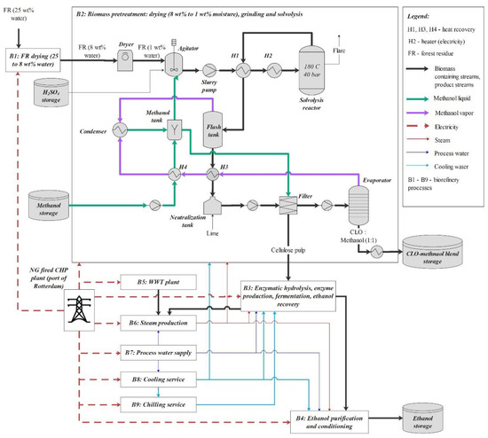
Figure 1.
Biomass pretreatment process—principal flow diagram and its integration into cellulosic ethanol biorefinery.
The slurry released after solvolysis is, first, flashed to atmospheric pressure allowing to recycle a part of methanol, then neutralized with quicklime and sent to a filter press. At the latter, CLO blended with methanol is separated from its solid fraction comprising mainly unconverted cellulose, solid lignin, and ash. In order to ensure a satisfactory solid separation, the filter press is coupled with a fresh methanol washing system, where additional methanol input is estimated based on the mass of cellulose in the pulp, namely 6:1. At the next step, CLO diluted in methanol is concentrated to a mass ratio of 1:1 in a settled downstream evaporator, and methanol vapour is condensed and recycled to the solvolysis section.
The cellulose pulp obtained through filtering is valorized to ethanol (99.5% purity) via subsequent enzymatic hydrolysis, fermentation, and ethanol conditioning. Design parameters for the cellulose conversion processes, as well as for enzyme production, wastewater treatment (WWT) plant, cooling and chilling facilities were derived from a model developed by NREL [23,24]. Cellulose-to-glucose and glucose-to-ethanol conversion rates were taken equal to 90% each. Steam is supplied from an on-site boiler that is, in the base scenario, fuelled by 6.1% with biogas produced internally, by 3.6% with solid residues and by 0.1% with WWT sludge, while the remaining energy deficit is covered by externally supplied bark-chips with LHV of 4.8 MJ/kg. The Vertoro biomass pretreatment process was designed in Aspen Plus® v.10 and integrated into the NREL model. The inventory of the biorefinery and FR supply models is provided in Table 1.

Table 1.
Biorefinery inventory for the production of 1 t of CLO.
2.3. Life Cycle Assessment and Economic Models
The life-cycle assessment (LCA) methodology was applied to evaluate the environmental profiles of the final products using the ISO 14,040 series methodology [25], with a system boundary set as well-to wheel/haul (Figure 2). Functional units were 1 GJ of CLO (excluding blending agent methanol) and 1 GJ of denatured ethanol, as recommended by the EU Renewable Energy Directive (RED) [26]. As an additional scenario for CLO, the functional unit of 1 tkm was deemed to be adequate to reflect the main function of freight transportation. The complete list of processes used in LCA is summarized in Table A1 of Appendix A.
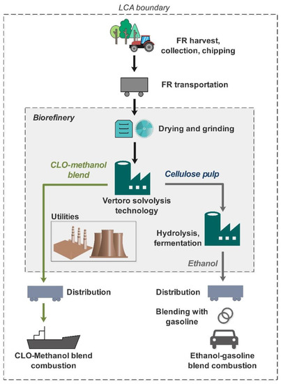
Figure 2.
Well-to-wheel/haul system boundary.
The allocation method for the base scenario, as recommended by RED, was based on the energy content [26]. To reflect the underlying physical relationship between material and energy inputs on one hand, and process outputs on the other, within the base scenario, methanol was regarded as a blending agent and excluded from the allocation (see Appendix A, Table A2 and Table A3). The allocation procedure was applied to a sub-divided product system following the methodology described in Obydenkova et al. [27,28].
The discounted cash-flow analysis was used to determine the minimum selling price (MSP) of CLO, where the latter reflected the price at the economic breakeven point.
The cost of equipment for biomass storage and handling, cellulose hydrolysis, fermentation, solids recovery and ethanol conditioning, as well as for enzyme production, WWT, boiler, process water supply and cooling sections were obtained using size factoring exponents m from the NREL report [24] and cost versus capacity relationship:
where subscripts “1” and “2” refer to equipment with a known purchase price and to that one for which costs are yet to be defined, respectively.
Cost2 = Cost1∙(Capacity2)/(Capacity1)m
Furthermore, the solid biomass handling equipment was added to the boiler section to take into account unloading and conveying bark chips. The cost of biomass pretreatment section was calculated based on price quotations from vendors for the 1 kt plant in Geleen. Additional direct and indirect costs were added to capital expenditures (CAPEX) to account for costs related to the site development, piping, warehouse, project contingency, etc. in line with the methodology described in the NREL report [24]. Numerical inputs to the economic model are summarized in Appendix B, Table A4.
Operational expenses included the costs of chemicals, materials and energy required to operate a biorefinery at its full capacity (see Appendix B, Table A5), as well as other fixed operational costs. Direct wages and benefits were calculated assuming five operators per shift, five shifts in total, as well as accounting for other required employees (see Appendix B, Table A6).
Assumptions on equity financing and depreciation schemes, while distinguishing between assets related to the cellulosic ethanol plant and those related to steam production, were taken similarly to those used in the NREL economic model [24]. All costs were converted into US dollars as of the project year 2021 using average plant cost indices as deflator [29].
The MSP of CLO was found iteratively by setting its value so as the project NPV is equal to zero.
2.4. Scenarios
Single point sensitivity analysis was conducted to evaluate the impact of the assumptions taken in the designed value chain on the environmental and economic profiles of biofuels. Table 2 summarizes the scenarios generated for this analysis.
Table 2.
Scenarios description and inputs to a single point sensitivity analysis.
2.4.1. Biorefinery Integration into the Energy Network
Infrastructure can have a significant impact on the environmental and economic performance of a biorefinery [28], which stresses the importance of an energy integration scenario analysis. Scenarios used in this analysis are summarized in Table 2.
Heat Network Integration
In the base scenario, it was assumed that the biorefinery uses bioenergy (bark-chips) to offset the thermal energy deficit caused by using lignin as biofuel.
Given possible limitations to the bark-chip supply, especially in line with the rising demand for green energy, two different energy integration options were analysed: (i) when the heat deficit is offset by steam supplied from a local natural gas-fired (NG-fired) CHP plant in Rotterdam [30], or (ii) when residual or waste heat sources are used for FR drying and methanol evaporation.
The impacts of heat produced at the NG-fired 400 MW CHP facility in The Netherlands, as well as of bark-chips at a consumer site in Europe, were retrieved from the Ecoinvent database [31], while the GHG emission associated with industrial waste heat that is regarded as a waste product from another industrial process was derived from a website providing Dutch CO2 emission factors [32].
The cost of steam produced from industrial waste heat was determined by different factors, including the temperature of flue gases, heat recovery system design, collection network and operational parameters. This paper utilized the range of costs of 1.16 to 4.13 €/t for saturated three-bar steam produced via a heat recovery steam generator from flue gases in such industries as cement, steel and silicon production and pulp and paper industry, located in Rotterdam [33].
Electricity Network Integration and Future Power Mix
In the base scenario, it was assumed that electricity was bought from the NG-fired 400 MW CHP plant located in Rotterdam [30]. However, the target set by The Netherlands Climate Act (May, 2019) will require the deep decarbonization of the energy sector, including power supply. While the share of renewables in the current Dutch electricity mix amounts to 12% [31], mainly from wind, this share will increase to 75% by 2030 [34]. Following this, an additional scenario using the Dutch 2030 electricity mix was set up to analyse the impact of power decarbonization on environmental profiles of CLO and ethanol. This mix was developed assuming proportional increase of the current shares of wind, solar and biomass-generated electricity in the total electricity mix, while decreasing the share of fossils.
The base power price used in this paper was taken to be equal to 125.2 $/MWh, that corresponds to The Netherlands 2021 average price for consumers [35], and the average of projected 2030 electricity prices at 42.2 $/MWh was taken for the scenario that involves power decarbonization solutions [36].
Methanol Origin
The base scenario assumed the use of fossil methanol for the biomass solvolysis process. However, due to the potential for the decarbonization of different economic activities via the use of methanol and an overall increase in the methanol demand, it was projected that, by the year 2050, the output of bio-methanol will exceed current, predominantly fossil, methanol production capacity by about one third [9]. Such capacity stands at 135 Mt of bio-methanol (obtained through biomass gasification), that is far below its potential taking into account biomass available, like waste and residues from forestry and agriculture, along with energy crops [9]. Thus, an additional scenario was set up to explore the opportunity of displacing the fossil methanol with the bio-based one. The environmental profile for the global distribution of bio-methanol, representing its production from biomass via the syngas route using the current energy and material mixes and its transportation, was retrieved from the Ecoinvent database [31].
The cost of fossil methanol was taken to be equal to 175 $/t, that is the average of current methanol prices, while the cost of bio-methanol at 734 $/t was the average from the reported bio-methanol price range assuming its production from a higher quality feedstock [9].
2.4.2. Technical Parameters Uncertainty
While technical parameters for the biomass pretreatment model were based on laboratory experiments and pilot tests at the Brightlands Chemelot Campus, which were batch based, the transition from batch processes to the continuous ones entailed further technological uncertainties that can alter environmental and economic results.
The degree of delignification (DL) of 95 wt%, one of the key technical parameters, was derived from laboratory experiments reported by Kouris et al. (2021) [12]. The magnitude of this parameter was dependent on the methanol-to-biomass ratio, acid loading and temperature, while under additional nitrogen pressure it fell within 50.2 and 98.8 wt%. Thus, the DL of 80 wt%, that is close to the median of the reported range, was taken for the sensitivity analysis.
The variance of the methanol-to-dry-FR mass ratio in the solvolysis section was assumed to lie within 3:1 and 7:1, i.e., within the ranges of ratios tested in laboratory. Additionally, a scenario representing a more advanced solid separation system was modelled, assuming the use of only a half of methanol required for the cellulose washing compared to the base scenario. Furthermore, two scenarios representing fossil and bio-methanol losses with cellulose pulp were modelled to evaluate the importance of methanol recovery in a biorefinery.
The modelling scenarios are summarized in Table 2.
2.4.3. Forest Residue Supply Chain Uncertainty
The main assumptions featuring a high level of uncertainty refer to the feedstock supply distance, moisture content of residues and the involvement of natural drying into the residue supply chain. Overall, four additional scenarios (Table 2) were established to test those uncertainties, including doubled delivery distance, 8 wt% and 50 wt% water content in residues and the omission of natural drying that is optionally compensated by container drying using the Dutch current power mix.
2.4.4. Methodological Uncertainty-Allocation Procedure
The allocation procedure can have a significant impact on the environmental profiles of biorefinery products imposing the necessity to test different allocation methods to decrease the related methodological uncertainty [27]. To that end, additional scenarios were set to analyse those impacts as summarized in Table 2.
There were two principally different groups of allocation methods, namely: one excluding blending agent, i.e., methanol, from the allocation procedure, and the other treating methanol as a part of the product. The default method was based on energy content, excluding methanol. Other methods include allocation based on the mass of valuable components (MVC), the total mass of flows, exergy content and economic value allocation. In the MVC method, burdens from the solvolysis section were partitioned based on the mass of cellulose in the pulp and the mass of C5 sugars and lignin oligomers in CLO, while burdens imposed by cellulose valorization processes were split based on the mass of ethanol and the combustible part of lignin residue (i.e., mass of the cake excluding water and ashes).
The inputs to allocation methods and allocation factors, as well as the details of the allocation procedure are summarized in Appendix A (Table A2 and Table A3).
2.5. Distribution of Biofuels and Biofuel Combustion
Given the intended final use, it was assumed that the distribution of CLO and ethanol follow the pattern of heavy fuel oil (HFO) and gasoline distribution mixes, respectively. Environmental profiles for those distribution mixes were derived from the Ecoinvent database [31].
Combustion emission factors for ethanol, methanol and gasoline were derived from the GREET® and GREET-marine® models [37,38], and converted to impact categories using specific characterization factors. Because of the lack of data related to emission factors for such GHG as nitrous oxide, as well as for NOx and CO emission from CLO combustion, the related scope of the analysis was narrowed down to fossil carbon dioxide and sulphur emissions, whose combustion emission factors were taken to be equal to zero based on the fossil carbon and sulphur content in lignin oil produced.
2.6. Dealing with Functionality
In the default model, the functional unit used for the analysis of the environmental footprint of CLO was based on energy as was recommended by RED. However, it did not consider volumetric energy densities of related fuels and cargo delivery logistics.
Although the CLO-methanol blend (1:1) and methanol have similar LHVs (20.2 MJ/kg versus 19.9 MJ/kg), their volumetric energy densities vary significantly (19.4 MJ/l versus 15.7 MJ/l). This difference can play a crucial role in the fuel storage on container ships and, subsequently, on the distance these ships can travel without refuelling. In the current paper, we have analysed how the difference in volumetric energy densities would affect such shipping patterns and associated carbon dioxide emissions per one tkm functional unit.
Following the methodology described in the GREET-marine® model [37], each trip was divided into three segments, which all have distinctive fuel consumption and emission factors due to different speed, load factors (i.e., portion of the rated engine power that is utilized during the process), and the use of either main or auxiliary engines. The container ship was assumed to travel in normal cruising conditions at the design speed of 39.21 km/h. This speed was lowered to 33.35 km/h during the transit through the reduced speed zones (RSZs). Those RSZs are often established near ports and allow limiting fuel consumption and emissions within the designated region. Finally, the time that the container ship spends at a dockside in the port of departure and arrival (dwell time, hoteling) was assumed to be 22 h. Additionally, an assumption concerning energy requirements for CLO-methanol blend-fired engine was taken like the one that involves methanol. The detailed input data and modelling approach are provided in the Supporting information.
2.7. Impact Assessment
For the analysis, the life cycle impact assessment (LCIA) methods recommended in the framework of the Environmental Footprint analysis [39,40] were used, which refer to the mid-point LCIA methods, namely: the climate change impact with a 100-year time horizon, particulate matter and respiratory inorganics impact, photochemical ozone formation, acidification and terrestrial eutrophication, marine aquatic eutrophication and the fossil fuels depletion.
The formula to calculate GHG emission saving from biofuels was adopted from RED [26]:
where EB is the total emissions from biofuel and EF is the fossil fuel comparator, representing its well-to-wheel GHG emissions.
Saving = (EF − EB)/EF
3. Results and Discussion
3.1. Base Scenario
3.1.1. Minimum Selling Price and Costs
The minimum selling price (MSP) of CLO was 846 $/t or 821 $/t of methanol equivalent (ME), thus falling within the range of the reported costs of the bio-methanol production of 455–1013 $/t when higher quality feedstock (6–15 $/GJ) is used [9].
Operational expenses amounted to about 60% of the total cost; of that figure the feedstock supply was responsible for 46%, chemicals and energy inputs for 29%, and wages, labour burden, maintenance, and property insurance together were responsible for 25% of those total expenses.
Concerning chemicals and energy inputs, steam production dominated these expenses with a share of 45%, followed by the group of carbohydrates valorization processes, at 20%, and biomass pretreatment process at 17%, while the WWT plant, feedstock drying, process water supply and cooling services altogether were responsible for the other 18% (Figure 3). Steam production was dominated by the cost of bark chips at 84%. Expenses related to the carbohydrate valorization processes were mainly determined by the cost of glucose at 63%, electricity at 28%; while 88% of expenses related to the biomass pretreatment process stem from the purchases of power.
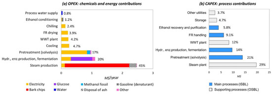
Figure 3.
Chemicals and energy contribution into operational expenses and installed equipment costs (ISBL—inside battery limits; OSBL—outside battery limits).
Capital investment, whose share in total costs amounts to 40%, was dominated by the steam production plant at 29%, biomass pretreatment at 21%, carbohydrates valorization at 14%, and WWT at 12%, see Figure 3. The forest residue handling, ethanol and solids recovery, storage, and utilities altogether were responsible for about 24% of the total installed equipment costs.
3.1.2. LCA Results
The global warming potential (GWP) of CLO at 14.8 kgCO2-eq/GJ exhibited an 84% GHG emission saving compared to fossil alternative, and it was more than half of that of bio-methanol (Figure 4). The CLO blend with fossil methanol (1:1) reduced GHG emission by 43.3% compared to the reference fuel. The significant improvement was also observed in the fossil fuel depletion potential (223 MJ/GJ) compared to both fossils and bio-methanol (1572 and 406 MJ/GJ, respectively).
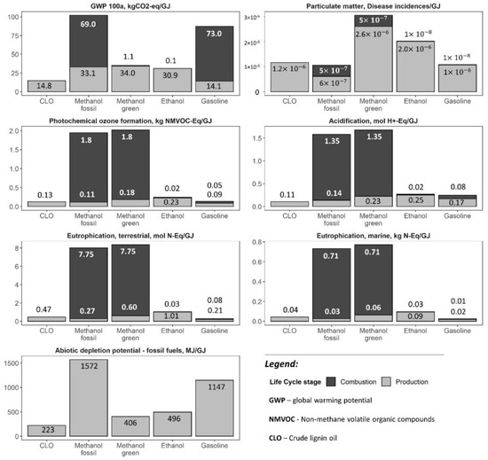
Figure 4.
LCA results-base scenario (this figure excludes combustion emissions of CLO).
There were four biorefinery processes responsible for about 75% of the climate change and fossil fuel depletion impacts of CLO, namely: biomass solvolysis at 30–34%, steam production at 19–20%, FR collection at 12–13%, and transportation at 12% (Figure 5). Those impacts were mainly attributable by 36–43% to the use of electricity, by 16–18% to bark chips for energy production and by 27–28% to diesel combustion during the FR supply and CLO distribution by heavy-duty vehicles (Figure 6). Concerning impacts associated with the import of electricity, 65% of such impacts were related to biomass pretreatment.
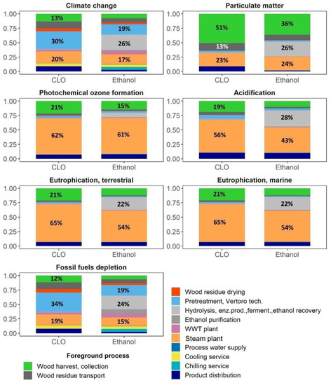
Figure 5.
Foreground processes contribution analysis.
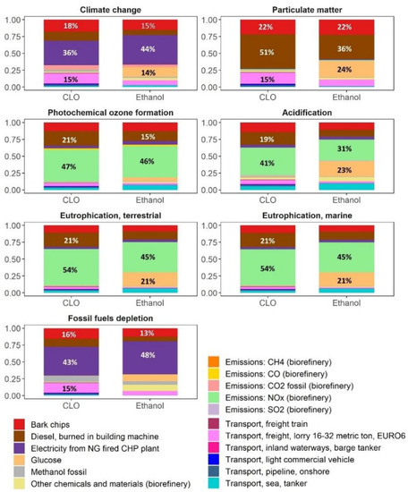
Figure 6.
Analysis of background processes and direct emissions contribution (the term “direct emissions” refer to air pollutants emitted directly during biorefinery operations).
The GWP of ethanol in the base scenario was 31.0 kgCO2-eq/GJ, i.e., resulting in a 67% GHG emission saving compared to the RED fossil fuel comparator. This impact was dominated by the complex of processes involved in the valorization of carbohydrates at 26% (Figure 5), mainly due to glucose and electricity, that was followed by biomass pretreatment at 19%, basically due to electricity, and energy production at 17% due to the use of bark chips. The overall share of electricity, glucose, and bark chips contribution to the climate change impact of ethanol amounted to 44%, 14% and 15%, respectively (Figure 6).
The impact of particulate matter of CLO on a human health of 1.1 × 10⁻⁶ disease/GJ was more than half of that for bio-methanol, while being approximately the same as of fossil methanol (Figure 4). However, while the impact of CLO and bio-methanol mainly stemmed from the production stage, for fossil methanol it was almost equally spread between the production and combustion stages. There were three main processes, all associated with the biomass supply, responsible for more than 85% of the particulate matter impact, with a contribution of FR harvest operations at 51%, bark chips used for steam production at 22% and FR transportation at 13% (Figure 5). The main contributors to the ethanol impact associated with particulate matter also stemmed from the use of bio-products, namely: FR harvest at 36%, glucose used in enzymatic hydrolysis at 24% and bark chips used for energy production at 22% (Figure 5 and Figure 6).
The impacts of CLO production on the photochemical ozone formation, 0.13 kg NMVOC-eq/GJ, acidification, 0.11 mol H+-eq/GJ, terrestrial and marine eutrophication, 0.47 mol N-eq/GJ and 0.04 kg N-eq/GJ, were in the range of those impacts for fossil and bio-methanol, while the main impact of methanol was associated with the combustion phase (Figure 4), mainly due to NOx emissions. The steam production section, mainly due to NOx emissions (42–54%) and FR harvest (19–21%), were among the main contributors to these impacts (Figure 5 and Figure 6). The related profiles of ethanol were additionally affected by the use of glucose for enzyme production (6–23%).
The omission of CLO combustion test results can be regarded to as one of the most important limitations of this paper around such health and environmental impacts as PM emissions, photochemical ozone formation, acidification, and eutrophication.
Although the said impacts of CLO were in the range of those reported for fossil and bio-methanol, overall methanol profile was dominated by the combustion phase, mainly due to NOx emissions, which have primarily the thermal origin. In the meantime, there was an evidence of a potential NOx combustion emission reduction using lignin derived oxygenates blends with diesel compared to pure diesel, that was mainly due to reduced LHV of the blend, and, as a result, the combustion temperature [41]. Thus, the similar NOx emission can be expected from methanol and CLO-methanol blends as having compatible LHV values.
3.2. Scenario Analysis
3.2.1. Biorefinery Integration into Infrastructure
The integration of the biorefinery under review into energy network may play a pivotal role in the climate change impact of both CLO and ethanol (Figure 7). Substituting steam produced from bark chips with that from the local NG-fired CHP plant (scenario I-2) showed the worst performance among all results, resulted in 20% and 17% GWP growth compared to the base scenario for CLO and ethanol, while the decarbonization of electricity (scenario I-3) will ensure the lowest GWP corresponding to its 20% and 23% reduction for CLO and ethanol, respectively.
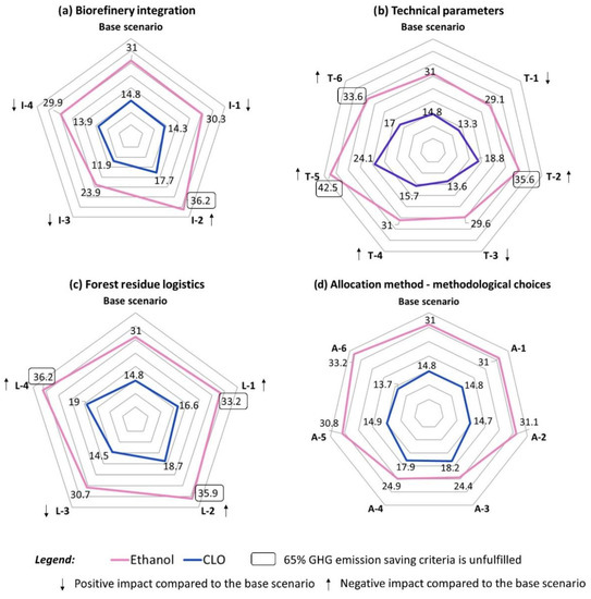
Figure 7.
GWP results-single point sensitivity analysis.
The displacement of fossil methanol using the bio-based one (scenario I-4), as well as using waste heat for FR drying and methanol evaporation (scenario I-1) had moderate positive impact on the GWP of both products, resulting in its reduction by 3 to 6% for CLO and by 2 to 4% for ethanol compared to the base scenario (Figure 7).
On the contrary, using waste heat for said processes, had the greatest CLO MSP reduction potential among other energy integration scenarios (Scenarios I-1-Low Price and I-1-High Price) of 33–35%, while using heat from an NG-fired CHP plant (scenario I-2) allowed a 15% MSP decrease compared to the base scenario (Figure 8). This MSP decrease stemmed mainly from the reduced CAPEX for the on-site steam production.
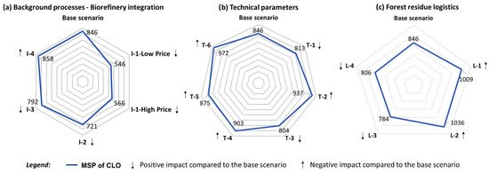
Figure 8.
Results of a single-point sensitivity analysis.
Using bio-methanol instead of the fossil one under basic technical assumptions had a rather immaterial effect on the lignin oil MSP, resulting in an about 1% growth in Scenario I-4.
A decrease in the base MSP by 6% in the scenario utilizing the 2030 electricity mix (Scenario I-3) was due to the fact that the 2021 average Dutch power price in the base scenario was almost three times of that projected for 2030, though the latter was expected to be strongly dependent on the price of fossil energy carriers [36].
Thus, the further valorization of the proposed solvolysis-based biorefinery concept might utilize the advantages of low boiling temperature solvents, such as methanol, entailing the opportunity to operate under the low-pressure saturated steam (about 3 bar), as that steam can be recovered from waste hot flue gases from e.g., cement, steel and other industries [33].
3.2.2. Sensitivity to Technical Parameters
For the biorefinery that used fossil methanol for solvolysis, additional methanol losses (scenario T-5), e.g., with cellulose pulp, had the highest impact on GWP of CLO and ethanol among other scenarios, resulting in its 63% and 37% growth, respectively (see Figure 7), while using bio-methanol (see Scenario T-6) can mitigate the consequences of additional methanol losses, that, however, was not enough for ethanol to meet the GHG emission saving criteria set by the RED. Additionally, using bio-methanol in that case (Scenario T-6) resulted in the highest among tested scenarios MSP exhibiting its growth by 15% compared to the base scenario (see Figure 8).
Both GWP and economic profiles of products will benefit from the reduction of methanol used in the biomass pretreatment. The decrease in the methanol-to-biomass ratio in the solvolysis reactor from 4:1 to 3:1 (scenario T-1) improved GWP of CLO and ethanol by 10% and 6%, respectively (Figure 7), and the MSP of CLO by 4% (Figure 8). The half-fold cut of the methanol-to-cellulose ratio in the filtration process (scenario T-3) will allow 5–8% GWP and 5% MSP reduction compared to the base case.
Conversely, the 7:1 ratio of the methanol-to-incoming biomass in the solvolysis reactor (scenario T-2) resulted in the increase of GWP of CLO and ethanol by 27% and 15%, respectively, and of lignin oil MSP by 11% that corresponded to the second highest ones among tested technical variables.
The decrease of DL in the solvolysis process from 95% to 80% (Scenario T-4) would have a modest negative impact, increasing its GWP and MSP by 6–7% (see Figure 7 and Figure 8). At the same time, a less efficient DL did not reflect on the GWP profile of ethanol that was due to more lignin becoming available for energy purposes, affecting positively ethanol value chain.
The obtained results point at the necessity to carefully evaluate, in line with the biorefinery upscaling, parameters favouring higher biomass loading, such as, for instance, pressure in the solvolysis rector. The recovery of methanol from cellulose pulp, unless it is not valorized downstream, would become another challenge to be resolved during that upscaling process. Options available for the latter might include, for instance, pulp drying with downstream methanol condensation or pulp washing with water.
3.2.3. Sensitivity to the Logistics of Forest Residues
The optimization of feedstock collection and delivery system might be needed to improve the environmental and economic profiles of CLO and ethanol. While the base scenario in this paper assumed the natural drying of FR, allowing to half its initial water content, this assumption might be strongly affected by seasonality. The assumption about natural drying of FR played a pivotal role in both the GWP and economic profiles of the products. Whenever natural drying was excluded (Scenarios L-2 and L-4), GWP increased by 26–28% for CLO and by 16–17% for ethanol vis-a-vis to the base assumption and the MSP of CLO for those scenarios was raised by 20–22% (see Figure 7 and Figure 8). At the same time, although using container drying at the collection point would decrease GHG emissions associated with its transportation to a biorefinery (due to a lower mass), it would not allow to offset the emissions imposed by the power consumed by electric fan, that was currently assumed to be the Dutch average power mix (Scenario L-4) (Figure 7). Hence, the transition of local suppliers to renewable electricity is another pivotal factor in the overall success of the valorization of FR towards biofuels.
The delivery distance of FR to a biorefinery was another main stressor of the CLO environmental and economic performance. With increased by a factor of two delivery distance, the GWP and MSP values lifted up by 12% and 20% compared to the base scenario, respectively (Figure 7 and Figure 8).
Figure 9 demonstrates Pareto front lines of main environmental impacts of FR transportation (i.e., GHG and PM emissions) and the corresponding MSP of CLO. In this figure, it was assumed that natural drying was not available. The results are presented regarding the Pareto preference order of minimal emissions and MSP, where the first and the last preference order refers to the best and the worst choice, respectively. These results highlight a trade-off between GHG and PM emissions imposed by the use of electricity to dry FR at the collection point, on one hand, and emissions imposed by FR transportation to a biorefinery, on the other. As a result, under the supply distance of about 160 km, any moisture content was acceptable to minimize environmental and economic dimensions, while at the distance of above 160 km, FR drying up to 8 wt% moisture was the only option to improve both economic and environmental profiles of the FR supply chain.
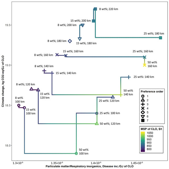
Figure 9.
The Pareto front lines for each Pareto preference order of minimal GHG and PM emissions and minimal MSP of CLO when natural drying is not available (the development of Pareto preference order follows the methodology described by Roocks [42], for the conditions when better tuples are required to be strictly better in all dimensions, i.e., for tuples t, t’ ∈ D, t < pt’ ∧ t < qt’ ∧ t < rt’, where p, q and r are preferences, such as GHG, PM and MSP).
3.2.4. Sensitivity to Allocation Methods
The allocation issue has been widely discussed by LCA practitioners [27,43,44]. In general, the consistency of results obtained via different allocation approaches points at their reliability [27].
By default, allocation based on energy content excluding the blending agent (methanol) was used to distribute GHG emissions between products, resulting in 14.8 and 31.0 kgCO2-eq per 1 GJ of CLO and ethanol, respectively (Figure 7). Nearly the same results were obtained using other allocation methods that exclude methanol, as well as via applying economic allocation (scenarios A-1, A-2, A-5, A-6). These scenarios resulted in the range of 13.7–14.9 kgCO2-eq/GJ for CLO and 30.8–33.2 kgCO2-eq/GJ for ethanol. Concerning the economic allocation, it should be noted that this method utilized production costs obtained in the current paper, rather than volatile market prices.
On the other hand, a good agreement was achieved between scenarios that include methanol in the allocation procedure (Scenarios A-3 and A-4). Those scenarios resulted in a higher impact associated with CLO (17.9–18.2 kgCO2-eq/GJ) and a significantly lower impact of ethanol (24.4–24.9 kgCO2-eq/GJ).
The discordance between these groups of allocation methods is supported by a similar observation concerning the inconsistency of LCA results obtained via two opposite allocation scenarios, including or excluding water from the allocation base [27]. The distortion observed might be highlighting the importance of the elimination of so called “dead” mass (e.g., blending agents, water) from the allocation procedure.
In multifunctional systems, like the current biorefinery, allocation procedures should be able to support another LCA goal aimed at the identification of “opportunities to improve the environmental performance of products” [25], that, however, requires establishing proper links between environmental stressors and individual environmental profiles of biorefinery products. From this perspective, the MVC allocation method appears more appropriate, as it allows, for instance, to reflect how the load of chemicals and enzymes affects the output of target products (i.e., CLO, cellulose, and ethanol). Noteworthy is that, in the current biorefinery, the MVC and energy content allocation methods, whereas the latter excludes methanol, showed identical results.
3.2.5. Biorefinery Capacity, Financing and Price Elasticity
Fixed capital investments (FCI) are the main factor having a significant impact on MSP of CLO. A 25% change of FCI causes an MSP response of about 20% (Figure 10), that also points at the impact the scale factor on the biorefinery economic feasibility of which is in an agreement with the observation made by Tschulkov et al. [45], highlighting the biorefinery scale being among decisive economic factors.
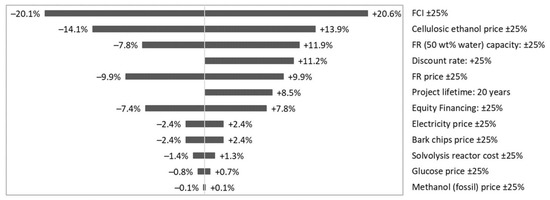
Figure 10.
Impact of biorefinery capacity, financing conditions and prices on the MSP of CLO.
Given the current cellulosic ethanol price is down by 25%, this will approach the minimum 2030 price estimate, and elevates MSP of CLO up by 14% (Figure 10). However, while the minimum 2030 ethanol price estimate stems from the assumption of a constant cost of feedstock, the future increasing competition for biomass could keep that price at the level of 1200 $/t in 2030 [46], close to the current price estimate adopted in the base scenario.
Figure 11 demonstrates the importance of the economy of scale for the biorefinery viability. Under a low cellulosic ethanol price of 805 $/t, which corresponds to the year 2030 low estimate, a biorefinery capacity below 91 kt (based on fresh FR) will not allow CLO to compete with bio-methanol.
Given the current cellulosic ethanol price hovering around 1220 $/t on the most important markets (e.g., Germany [47]), a biorefinery capacity of above 62 kt will be required to produce competitive lignin oil, which, with the refinery capacity going up to 250 kt, will result in MSP of $614 per ton of ME that subsequently allows falling under the medium price estimate for bio-methanol. With cellulosic ethanol prices above 1750 $/t, the capacity exceeding 215 kt based on fresh FR will ensure the production of CLO at a cost of below 455 $/t, the current lowermost cost estimate of bio-methanol production (Figure 11).
Discount rate is the fourth factor by magnitude causing an MSP response of above 10 percent (Figure 10).
Concerning the FR price, if it is up by 25%, this will be an equivalent of 10 $/GJ and persisting at the highest point of reported Dutch forest residue [48,49]. The impact of that price on MSP of CLO can be also regarded to as significant, lifting MSP of CLO by approximately 10%.
The response of CLO MSP to other parameters and price volatility was observed at a level of below 9%.
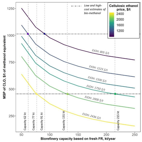
Figure 11.
MSP of CLO as a function of a biorefinery capacity and cellulosic ethanol price. The six- tenths rule was applied to approximate the cost of equipment at different biorefinery capacities. Current price of bio-methanol corresponds to feedstock cost at 6–15 $/GJ [9]; cellulosic ethanol prices of 805 $/t, 1223 $/t and 2436 $/t correspond to the 2030 low estimate [46], 2021 average price and end-of-May 2022 Swedish ethanol price [50], respectively.
3.3. Biorefinery Capacity and Shipping
The higher volumetric energy density enables a CLO-methanol-propelled vessel to travel 3347–4463 km (23.9%) further than if it was fuelled with methanol. In other words, when a panamax ship with a cargo capacity of 4818 twenty-foot equivalent unit (TEU) fuelled with the CLO-methanol blend leaves the port of Rotterdam, it can reach the port of Shanghai in China, which is 19,535 km away without refuelling, while the same container ship propelled with methanol, will have to hotel in the port of Bangkok in Thailand to refuel on its way to China.
Due to these cruising distances and vessel dwell time in ports, when an auxiliary engine is used, the fuel consumption and related emissions per unit of tonne-kilometre further decrease, though not significantly. The specific fuel consumption of the CLO-methanol blend and methanol were found to be 7.05 g/tkm and 7.17 g/tkm, respectively, that corresponds to engine carbon dioxide emission of 4.74 and 9.63 gCO2/tkm.
The travelling time of a panamax ship from the port of Rotterdam to the port of Shanghai amounts to 22.6 days with the total CLO-methanol blend (1:1) consumption of 6.098 kt per one-way trip that corresponds to 8.7 of such trips per year possible at a given annual biorefinery CLO capacity. The detailed results are provided in the Supporting information.
4. Conclusions
Lignocellulosic biofuels that can be blended with methanol offer a potential to improve the lifecycle emission of such blends and can be regarded as a short- to mid-term pathway towards climate neutral shipping.
The study presents a novel lignin valorization route towards marine fuel based on a biomass solvolysis pretreatment technology developed by Vertoro, a Dutch company, and analyses the GHG emission profile and economic value of such fuel. This concept includes the valorization of lignin to crude lignin oil (CLO) as a marine biofuel, and cellulose to ethanol.
The co-production of CLO and ethanol allows to achieve a more than 65% GHG emission saving compared to fossil fuels; thus, these biofuels fulfil the GHG emission saving criteria set by the EU Renewable Energy Directive. The CLO can be produced at the minimum selling price of 821 $/t of methanol equivalent that can be further decreased to $530–$549 with the use of low-pressure steam from waste heat sources for forest residues drying and methanol evaporation.
There are four main hotspots related to lignin oil value chain, namely: steam production, biomass pretreatment, forest residue harvest, collection, and transportation to a biorefinery, contributing to more than 75% of climate change and fossil fuel depletion impact categories. The steam plant, with its share of 56–65%, also dominates the photochemical ozone formation, acidification, and eutrophication, while forest residue harvest and collection contribute to 43–64% of particulate matter impact.
The sustainable co-production of CLO and cellulosic ethanol might require comprehensive measures to overcome identified hotspots and to improve the value chain of the biofuels furthermore. Pilot tests should carefully evaluate the possibility of decreasing the amount of methanol in the solvolysis section, as well as methanol losses and its recovery in the biorefinery. The decarbonization of electricity will play a pivotal role in improving climate change and fossil fuel depletion impact, as this would enable CLO and ethanol to reach a GHG emission saving of 75–87%.
Given a delivery distance of forest residue exceeding 160 km, the optimization of the supply chain shall include options for residue drying to below 10 wt% moisture at the collection site. However, if forced drying is an issue while natural drying is not available, the use of renewable electricity to that end will be crucial to reach a satisfactory GHG emission saving criteria.
Concerning methodological choices, the importance of testing different allocation methods should be noted. In this paper, we found a major disagreement in the results, of about 20%, between the groups of scenarios that included and those that did not include methanol, i.e., the blending agent, into the allocation procedure.
Combustion tests on CLO shall be performed to decrease the uncertainty connected to engine emissions contributing to such impacts as particulate matter, photochemical ozone formation, acidification, and eutrophication.
Supplementary Materials
The following supporting information can be downloaded at https://www.mdpi.com/article/10.3390/en15145007/s1: Transportation of cargo-model.
Author Contributions
Conceptualization, S.V.O.; methodology, S.V.O. and L.V.E.D.; software, S.V.O.; validation, S.V.O. and L.V.E.D.; formal analysis, S.V.O. and L.V.E.D.; resources, D.M.J.S. and Y.v.d.M.; data curation, S.V.O.; writing—original draft preparation, S.V.O. and L.V.E.D.; writing—review and editing, P.D.K. and Y.v.d.M.; visualization, S.V.O.; supervision, M.D.B., D.M.J.S. and Y.v.d.M.. All authors have read and agreed to the published version of the manuscript.
Funding
This research received no external funding.
Data Availability Statement
Not applicable.
Conflicts of Interest
The authors declare no conflict of interest.
Nomenclature
| AF | allocation factor |
| CAPEX | capital expenditures |
| CHP | combined heat and power |
| CLO | crude lignin oil |
| DL | degree of delignification |
| FCI | fixed capital investments |
| FR | forest residue |
| GHG | greenhouse gases |
| GWP | global warming potential |
| ISO | the International Organization for Standardization |
| LCA | life-cycle assessment |
| LHV | lower heating value |
| ME | methanol equivalent |
| MSP | minimum selling price |
| MVC | mass of valuable components |
| NMVOC | non-methane volatile organic compounds |
| NPV | net present value |
| NREL | the National Renewable Energy Laboratory |
| PM | particulate matter |
| RED | EU Renewable Energy Directive |
| TEU | twenty-foot equivalent unit |
Appendix A
Appendix A.1. LCA–Background Processes
System boundaries, geography, and system modelling approach for the LCA background processes are provided in Table A1.
Table A1.
Background processes for the LCA model.
Table A1.
Background processes for the LCA model.
| Product/Activity | System Boundary | Geography * | System Model |
|---|---|---|---|
| Chemicals and materials | |||
| Methanol fossil | Market for methanol | GLO | Allocation, cut-off by classification |
| Bio-methanol | Market for methanol | RoW | Allocation, cut-off by classification |
| Sulphuric acid | Market for sulphuric acid | RER | Allocation, cut-off by classification |
| Sodium hydroxide to generic market for neutralizing agent | Market for neutralizing agent | GLO | Allocation, cut-off by classification |
| Corn steep liquor (of project US life cycle inventory database) | Production | RNA | Allocation, cut-off by classification |
| Diammonium phosphate | Market for diammonium phosphate | RER | Allocation, cut-off by classification |
| Glucose | Market for glucose | GLO | Allocation, cut-off by classification |
| Ammonia anhydrous, liquid | Market for ammonia anhydrous, liquid | RER | Allocation, cut-off by classification |
| Sulphur dioxide, liquid | Market for sulphur dioxide, liquid | RER | Allocation, cut-off by classification |
| Quicklime, milled, packed | Market for quicklime, milled, packed | RER | Allocation, cut-off by classification |
| Gasoline (denaturant) | Market for petroleum | GLO | Allocation, cut-off by classification |
| Water, completely softened | Market for water, completely softened | RER | Allocation, cut-off by classification |
| Bark chips, wet, measured as dry mass | Market for bark chips, wet, measured as dry mass | Europe without Switzerland | Allocation, cut-off by classification |
| Diesel, burned in building machine | Market for diesel, burned in building machine | GLO | Allocation, cut-off by classification |
| Heavy fuel oil | Market group for heavy fuel oil | RER | Allocation, cut-off by classification |
| Energy supply | |||
| Electricity, medium voltage | Market for electricity, medium voltage | NL | Allocation, cut-off by classification |
| Electricity - heat and power co-generation, natural gas, conventional power plant, 400 MW | Production | NL | Allocation, cut-off by classification |
| Heat- heat and power co-generation, natural gas, conventional power plant, 400 MW | Production | NL | Allocation, cut-off by classification |
| Transportation | |||
| Transport, freight, lorry 16–32 metric ton, EURO6 | Market for transport, freight, lorry 16–32 metric ton, EURO6 | RER | Allocation, cut-off by classification |
| Transport, freight, sea, tanker for petroleum | Market for transport, freight, sea, tanker for petroleum | GLO | Allocation, cut-off by classification |
| Transport, pipeline, onshore, petroleum | Market for transport, pipeline, onshore, petroleum | RER | Allocation, cut-off by classification |
| Transport, freight train | Market group for transport, freight train | RER | Allocation, cut-off by classification |
| Transport, freight, inland waterways, barge tanker | Market for transport, freight, inland waterways, barge tanker | RER | Allocation, cut-off by classification |
| Transport, freight, light commercial vehicle | Market group for transport, freight, light commercial vehicle | RER | Allocation, cut-off by classification |
* GLO–average global production; RER–Europe; RoW–rest of the world; RNA—Region North America; NL—The Netherlands.
Appendix A.2. Allocation Methods
The current study evaluates such allocation methods as energy and exergy content (excluding and including blending agent), mass of valuable components (MVC), the total mass (excluding and including blending agent) and economic value. Allocation factors (AF) for these methods, except for MVC one, were found using the next equation:
where Fi refers to either energy or exergy content of flow i, or to its mass, or to the cost.
AF = (Fi/∑Fi)·100%
The energy content of a flow is defined based on its lower heating value (LHV):
where m is a mass of an ith product-stream.
Fi = mi LHVi
The costs of CLO and intermediate products, i.e., cellulose pulp, diluted ethanol and lignin residue were calculated using methodology described by Obydenkova et al. [28], and the base allocation method was used to that end. These costs, however, exclude labour and land related costs, as well as working capital, depreciation and taxes.
Allocation based on MVC utilizes the mass of cellulose, C5 sugars and lignin oligomers to partition burdens after solvolysis section and in the mass of ethanol and combustible part of the lignin cake (i.e., mass of the cake excluding water and ashes) after ethanol recovery section:
where AF(MVC) is allocation factor obtained via MVC method; subscripts CP, CLO, DE and LR refer to cellulose pulp, crude lignin oil, diluted ethanol, and lignin residue, respectively; w is a mass fraction.
AFCP(MVC) = (mcellulose in CP/(mcellulose in CP + mlignin oligomers in CLO + mC5 sugars in CLO)) × 100%
AFCLO (MVC) = ((mlignin oligomers in CLO + mC5 sugars in CLO)/(mcellulose in CP + mlignin oligomers in CLO + mC5 sugars in CLO)) ×100%
AFDE (MVC) = (methanol in DE/(methanol in DE + mLR (1 − wH2O in LR − wash in LR))) 100%
AFLR (MVC) = (mLR (1 − wH2O in LR − wash in LR)/(m ethanol in DE + mLR (1 − wH2O in LR − wash in LR))) × 100%
Allocation method based on exergy content includes both physical (Eph) and chemical (Ech) exergy, which were found using the next equations:
where h and s are the specific mass enthalpy and entropy of a flow, respectively; T is a temperature; subscript “0” refers to the reference conditions (25 °C and 1 atm); echi is the specific molar chemical exergy of substance i and Mi is its molecular weight.
Eph = [(h − h0) − T0·(s − s0)]·m
Echi = Σ(echi/Mi)·mi
Specific molar chemical exergy was defined using the equation from [51]:
where g is Gibbs function at the reference conditions (25 °C and 1 atm); n are stoichiometric coefficients in the fuel combustion reaction; echCO2, echH2O(l), echO2, echN2, echSO2 are standard chemical exergies (water in a liquid state); subscript “F” refers to the fuel in question.
ech = [gF + nO2·gO2 − nCO2·gCO2 − nH2O·gH2O(l) − nN2·gN2− nSO2·gSO2] +
[nCO2·echCO2 + nH2O·echH2O(l) + nN2·echN2 + nSO2·echSO2 − nO2·echO2]
[nCO2·echCO2 + nH2O·echH2O(l) + nN2·echN2 + nSO2·echSO2 − nO2·echO2]
Table A2.
Inputs to allocation procedure.
Table A2.
Inputs to allocation procedure.
| Product * | Mass, kg/h | LHV, MJ/kg | Cost, $/t |
|---|---|---|---|
| CP | 2765 | 15.5 | 376 |
| CLO, excluding methanol | 3164 | 20.5 | 510 |
| CLO, including methanol | 6265 | 20.0 | - |
| DE | 2371 | 13.3 | 687 |
| LR | 681.6 | 2.92 | 141 |
| CLO-methanol blend composition (wt%): | |||
| Lignin oligomers and C5 sugars | 49.5 | ||
| Methanol | 49.5 | ||
| Water | 1.00 | ||
| CP composition (wt%): | |||
| Cellulose | 93.0 | ||
| Lignin | 3.0 | ||
| Ash | 4.0 | ||
| DE composition (wt%): | |||
| Ethanol | 50.0 | ||
| Water | 50.0 | ||
| LR composition (wt%): | |||
| Water | 35.1 | ||
| Ash | 22.5 | ||
| Lignin | 11.6 | ||
| Cellulose | 17.5 | ||
| Glucose | 0.15 | ||
| Lactic acid | 0.27 | ||
| Other combustible compounds | 12.9 | ||
| Standard chemical exergy (ech) at 25°C and 1 atm, kJ/mol: | |||
| Sulphur dioxide (SO2) | 313.4 | ||
| Oxygen (O2) | 3.97 | ||
| Nitrogen (N2) | 0.72 | ||
| Carbon dioxide | 19.87 | ||
| Water (liquid) | 0.9 | ||
| Gibbs function of formation (g) at 25°C and 1 atm, kJ/mol: | |||
| Lignin | −267.1 | ||
| Xylan | −721.3 | ||
| Cellulose | 2.38 × 10⁻¹³ | ||
| Glucose | −930.5 | ||
| Ethanol | −174.2 | ||
| Lactic acid | −526.4 | ||
| Sulphur dioxide (SO2) | −300.1 | ||
| Oxygen (O2) | 0 | ||
| Nitrogen (N2) | 0 | ||
| Carbon dioxide | −394.4 | ||
| Water | −237.2 | ||
* CP—cellulose pulp; CLO—crude lignin oil; DE—diluted ethanol; LR—moist lignin residue.
Table A3.
Allocation factors.
Table A3.
Allocation factors.
| Process | Product * | Allocation Method and Scenario | ||||||
|---|---|---|---|---|---|---|---|---|
| Energy, Excl. Methanol (Base Scenario) | MVC (Scenario A-1) | Total Mass Excl. Methanol (Scenario A-2) | Total Mass Incl. Methanol (Scenario A-3) | Energy, Incl. Methanol (Scenario A-4) | Economic Value (Scenario A-5) | Exergy, Excl. Methanol (Scenario A-6) | ||
| Biomass pretreatment | CP | 39.8% | 45.3% | 46.6% | 30.6% | 25.5% | 39.2% | 47.2% |
| CLO | 60.2% | 54.7% | 53.4% | 69.4% | 74.5% | 60.8% | 52.8% | |
| Ethanol recovery | DE | 94.1% | 80.4% | 77.7% | 77.7% | 94.2% | 94.4% | 88.1% |
| LR | 5.9% | 19.6% | 22.3% | 22.3% | 5.8% | 5.6% | 11.9% | |
* CP—cellulose pulp; CLO—crude lignin oil; DE—diluted ethanol; LR—moist lignin residue.
Appendix B
Inputs to the economic model and materials, chemicals and energy prices are provided in Table A4 and Table A5.
Table A4.
Inputs to economic model.
Table A4.
Inputs to economic model.
| Description | Unit | Base Value | Ref. |
|---|---|---|---|
| Installed equipment cost | |||
| Biomass handling | M$ | 6.1 | [24] |
| Biomass pretreatment (solvolysis) | M$ | 13.9 | Vendor quotations and own calculations |
| Enzymatic hydrolysis, fermentation | M$ | 6.4 | [24] |
| Enzyme production | M$ | 3.1 | [24] |
| Ethanol, solids recovery and ethanol conditioning | M$ | 3.9 | [24] |
| WWT plant | M$ | 8.2 | [24] |
| Steam production | M$ | 19.6 | [24] |
| Process water supply, cooling, and chilling services | M$ | 2.5 | [24] |
| Ethanol and CLO storage | M$ | 3.2 | [24] |
| Annual operational expenses | |||
| Cost of feedstock | M$ | 8.9 | Calculated |
| Cost of chemicals, energy, and materials, excluding feedstock | M$ | 5.5 | Calculated |
| Fixed operating costs (wages, labour burden, maintenance, insurance) | M$ | 4.8 | Calculated |
| Depreciation | |||
| Biorefinery | |||
| Declining balance rate | % | 200 | [24] |
| Recovery period | years | 7 | [24] |
| Steam production | |||
| Declining balance rate | % | 150 | [24] |
| Recovery period | years | 20 | [24] |
| Annual production | |||
| CLO | kt | 26.6 | Calculated |
| Cellulosic ethanol | kt | 10.3 | Calculated |
| General | |||
| Project year | year | 2021 | - |
| Number of operating hours | h/year | 8410 | [24] |
| Discount rate | % | 10 | [24,52] |
| Equity Financing | % | 40 | [24] |
| Number of years for loan | % | 10 | [24] |
| Construction period | years | 3 | [24] |
| Start-up time | months | 3 | [24] |
| Corporate income tax rate | % | 25 | [53] |
Table A5.
Materials, chemicals and energy prices.
Table A5.
Materials, chemicals and energy prices.
| Input | Unit | Base Scenario | Ref. |
|---|---|---|---|
| Chemicals and material prices | |||
| Methanol fossil | $/t | 175 | [9] |
| Bio-methanol | $/t | 734 | [9] |
| Glucose | $/t | 712 | [24] |
| Cellulosic ethanol | $/t | 1223 | [46,47] |
| FR at biorefinery gate (25 wt% moisture) | $/t | 137 | Calculated based on data from [22,49] |
| Bark chips | $/GJ | 5 | [9] |
| Sulphuric acid | $/t | 110 | [24] |
| Corn steep liquor | $/t | 108 | [24] |
| Diammonium phosphate | $/t | 1298 | [24] |
| Ammonia | $/t | 550 | [24] |
| Sulphur dioxide | $/t | 428 | [24] |
| Cellulase nutrient mix | $/t | 1007 | [24] |
| Sorbitol | $/t | 1481 | [24] |
| Boiler chemicals | $/t | 6126 | [24] |
| Cooling tower chemicals | $/t | 3671 | [24] |
| Disposal of ash | $/t | 39 | [24] |
| Calcium oxide | $/t | 77 | Calculated based on data from [31] |
| Calcium hydroxide | $/t | 245 | [24] |
| Gasoline | $/t | 222 | [35] |
| Water | $/t | 0.311 | [24] |
| Energy prices | |||
| Electricity price 2021 | $/MWh | 125.2 | [35] |
| Low pressure steam (3 bar) | $/MJ | 6.84∙10−4 (min) 2.44∙10−3 (max) | Calculated based on data from [33] |
| Steam from natural gas | $/MJ | 1.59∙10−2 | [35] |
Table A6.
Labour requirements.
Table A6.
Labour requirements.
| Position | Number of Employees |
|---|---|
| Plant manager | 1 |
| Plant engineer | 1 |
| Maintenance supervisor | 1 |
| Maintenance technician | 1 |
| Lab manager | 1 |
| Lab technician | 2 |
| Shift supervisor | 5 |
| Shift operator | 25 |
| Yard employee | 1 |
| Clerk, secretary | 1 |
References
- International Transport Forum. ITF Transport Outlook 2019; OECD: Paris, France, 2019. [Google Scholar] [CrossRef]
- Hsieh, C.-W.C.; Felby, C. Biofuels for the Marine Shipping Sector; IEA Bioenergy: Copenhagen, Denmark, 2017; Available online: https://www.ieabioenergy.com/wp-content/uploads/2018/02/Marine-biofuel-report-final-Oct-2017.pdf (accessed on 12 June 2022).
- International Transport Forum. ITF Transport Outlook 2021; OECD: Paris, France, 2021. [Google Scholar] [CrossRef]
- International Energy Agency. Energy Technology Perspectives 2020; IEA: Paris, France, 2020; Available online: https://www.iea.org/reports/energy-technology-perspectives-2020 (accessed on 6 June 2022).
- Initial IMO Strategy on Reduction of GHG Emissions from Ships. 2018. Available online: https://wwwcdn.imo.org/localresources/en/OurWork/Environment/Documents/Resolution%20MEPC.304%2872%29_E.pdf (accessed on 6 June 2022).
- European Environment Agency. European Maritime Transport Environmental Report 2021; EEA: Copenhagen, Denmark, 2021. [Google Scholar] [CrossRef]
- Forsyth, A. All at Sea—Methanol and Shipping. 2022. Available online: https://www.methanol.org/wp-content/uploads/2022/01/Methanol-and-Shipping-Longspur-Research-25-Jan-2022.pdf (accessed on 6 June 2022).
- Methanol as an Alternative Fuel for Vessels. 2018. Available online: https://sustainableworldports.org/wp-content/uploads/MKC-TNO-and-TU-Delft_2018_Methanol-as-an-alternative-fuel-for-vessels-report.pdf (accessed on 6 June 2022).
- Innovation Outlook: Renewable Methanol; IRENA: Abu Dhabi, United Arab Emirates, 2021; Available online: https://www.irena.org/-/media/Files/IRENA/Agency/Publication/2021/Jan/IRENA_Innovation_Renewable_Methanol_2021.pdf (accessed on 6 June 2022).
- Raj, T.; Chandrasekhar, K.; Naresh Kumar, A.; Rajesh Banu, J.; Yoon, J.J.; Kant Bhatia, S.; Yang, Y.H.; Varjani, S.; Kim, S.H. Recent advances in commercial biorefineries for lignocellulosic ethanol production: Current status, challenges and future perspectives. Bioresour. Technol. 2022, 344, 126292. [Google Scholar] [CrossRef] [PubMed]
- Obydenkova, S.V.; Kouris, P.; Hensen, E.J.M.; Heeres, H.J.; Boot, M.D. Environmental economics of lignin derived transport fuels. Bioresour. Technol. 2017, 243, 589–599. [Google Scholar] [CrossRef] [PubMed]
- Kouris, P.D.; Huang, X.; Ouyang, X.; van Osch, D.J.G.P.; Cremers, G.J.W.; Boot, M.D.; Hensen, E.J.M. The impact of biomass and acid loading on methanolysis during two-step lignin-first processing of birch wood. Catalysts 2021, 11, 750. [Google Scholar] [CrossRef]
- Vertoro Takes Step towards Large-Scale Production of ‘Green Oil’ in a Pilot Plant. Available online: https://www.tue.nl/en/news/news-overview/29-06-2020-vertoro-takes-step-towards-large-scale-production-of-green-oil-in-a-pilot-plant/ (accessed on 5 April 2022).
- Whittaker, C.; Mortimer, N.; Murphy, R.; Matthews, R. Energy and greenhouse gas balance of the use of forest residues for bioenergy production in the UK. Biomass Bioenergy 2011, 35, 4581–4594. [Google Scholar] [CrossRef] [Green Version]
- Vonk, M.; Theunissen, M. The Harvest of Logging Residues in the Dutch Forests and Landscape. 2007. Available online: https://www.probos.net/biomassa-upstream/pdf/finalmeetingpaperharvestofloggingresidues.pdf (accessed on 15 January 2022).
- Han, J.E.A.; Palou-Rivera, I.; Dunn, J.B.; Wang, M.Q. Well-to-Wheels Analysis of Fast Pyrolysis Pathways with GREET; Argonne National Laboratory: Lemont, IL, USA, 2011. Available online: https://greet.es.anl.gov/publication-wtw_fast_pyrolysis (accessed on 5 April 2022).
- Phyllis2 Database. Available online: https://phyllis.nl/Browse/Standard/ECN-Phyllis#pine%20wood (accessed on 17 October 2021).
- Elsayed, M.A.; Matthews, R.; Mortimer, N.D. Carbon and Energy Balances for a Range of Biofuels Options; Resources Research Unit Sheffield Hallam University: Sheffield, UK, 2003. Available online: https://www.osti.gov/etdeweb/servlets/purl/20359706 (accessed on 30 January 2021).
- Wang, J.; Gao, J.; Brandt, K.L.; Wolcott, M.P. Energy consumption of two-stage fine grinding of Douglas-fir wood. J. Wood Sci. Off. J. Jpn. Wood Res. Soc./Jpn. Wood Res. Soc. 2018, 64, 338–346. [Google Scholar] [CrossRef] [Green Version]
- Nordhagen, E. Drying of Wood Chips with Surplus Heat from Two Hydroelectric Plants in Norway. 2011. Available online: http://citeseerx.ist.psu.edu/viewdoc/download?doi=10.1.1.1075.1756&rep=rep1&type=pdf (accessed on 6 June 2022).
- De Kam, M.J.; Vance Morey, R.; Tiffany, D.G. Biomass Integrated Gasification Combined Cycle for heat and power at ethanol plants. Energy Convers. Manag. 2009, 50, 1682–1690. [Google Scholar] [CrossRef]
- Meulen, S.V.D.; Grijspaardt, T.; Mars, W.; Geest, W.V.D.; Roest-Crollius, A.; Kiel, J. Cost Figures for Freight Transport—Final Report. 2020. Available online: https://www.kimnet.nl/publicaties/formulieren/2020/05/26/cost-figures-for-freight-transport (accessed on 10 April 2022).
- Davis, R.; Tao, L.; Scarlata, C.; Tan, E.C.D.; Ross, J.; Lukas, J.; Sexton, D. Process Design and Economics for the Conversion of Lignocellulosic Biomass to Hydrocarbons: Dilute-Acid and Enzymatic Deconstruction of Biomass to Sugars and Catalytic Conversion of Sugars to Hydrocarbons; NREL/TP-5100-62498; National Renewable Energy Lab. (NREL): Golden, CO, USA, 2015. Available online: https://www.osti.gov/servlets/purl/1176746 (accessed on 6 June 2022)NREL/TP-5100-62498.
- Humbird, D.; Davis, R.; Tao, L.; Kinchin, C.; Hsu, D.; Aden, A.; Schoen, P.; Lukas, J.; Olthof, B.; Worley, M.; et al. Process Design and Economics for Biochemical Conversion of Lignocellulosic Biomass to Ethanol: Dilute-Acid Pretreatment and Enzymatic Hydrolysis of Corn Stover; NREL/TP-5100-47764; National Renewable Energy Lab. (NREL): Golden, CO, USA, 2011. Available online: https://www.osti.gov/servlets/purl/1013269 (accessed on 6 June 2022).
- ISO 14040:2006; Environmental Management—Life Cycle Assessment—Principles and Framework. ISO: Geneva, Switzerland, 2006. Available online: https://www.iso.org/obp/ui/#iso:std:iso:14040:ed-2:v1:en (accessed on 6 June 2022).
- Directive (EU) 2018/2001 of the European Parliament and of the Council of 11 December 2018 on the Promotion of the Use of Energy from Renewable Sources (Recast) (Text with EEA Relevance). 2018. Available online: https://eur-lex.europa.eu/eli/dir/2018/2001/oj#d1e32-147-1 (accessed on 6 June 2022).
- Obydenkova, S.V.; Kouris, P.D.; Smeulders, D.M.J.; Boot, M.D.; Meer, Y. Modeling life-cycle inventory for multi-product biorefinery: Tracking environmental burdens and evaluation of uncertainty caused by allocation procedure. Biofuels Bioprod. Biorefining 2021, 15, 1281–1300. [Google Scholar] [CrossRef]
- Obydenkova, S.V.; Kouris, P.D.; Smeulders, D.M.J.; Boot, M.D.; Meer, Y. Evaluation of environmental and economic hotspots and value creation in multi-product lignocellulosic biorefinery. Biomass Bioenergy 2022, 159, 106394. [Google Scholar] [CrossRef]
- Plant Cost Index. Available online: https://www.chemengonline.com/site/plant-cost-index/ (accessed on 5 April 2022).
- Enecogen. Welcome to Enecogen. Available online: https://enecogen.nl/en/general-information/ (accessed on 21 February 2022).
- Ecoinvent v.3.8. Available online: https://ecoinvent.org/the-ecoinvent-database/ (accessed on 1 May 2022).
- CO2 Emissiefactoren. Lijst Emissiefactoren. Available online: https://www.co2emissiefactoren.nl/lijst-emissiefactoren/ (accessed on 21 February 2022).
- Ali, H.; Eldrup, N.H.; Normann, F.; Andersson, V.; Skagestad, R.; Mathisen, A.; Øi, L.E. Cost estimation of heat recovery networks for utilization of industrial excess heat for carbon dioxide absorption. Int. J. Greenh. Gas Control 2018, 74, 219–228. [Google Scholar] [CrossRef]
- Hammingh, P.; Daniels, B.; Koutstaal, P.; Schure, K.; Hekkenberg, M.; Menkveld, M. Netherlands Climate and Energy Outlook 2020 Summary. 2020. Available online: https://www.pbl.nl/sites/default/files/downloads/pbl-2020-netherlands-climate-and-energy-outlook-2020-summary-4299.pdf (accessed on 5 April 2022).
- StatLine. Available online: https://www.cbs.nl/en-gb (accessed on 6 April 2022).
- Afman, M.; Hers, S.; Scholten, T. Energy and Electricity Price Scenarios 2020–2023–2030. Input to Power to Ammonia Value Chains and Business Cases. 2017. Available online: https://cedelft.eu/wp-content/uploads/sites/2/2021/04/CE_Delft_3H58_Energy_and_electricity_price_scenarios_DEF.pdf (accessed on 5 April 2022).
- ANL. Life Cycle Analysis of Conventional and Alternative Marine Fuels in GREET™. 2013. Available online: https://greet.es.anl.gov/publication-marine-fuels-13 (accessed on 5 April 2022).
- GREET® Model. The Greenhouse Gases, Regulated Emissions, and Energy Use in Technologies Model. Available online: https://greet.es.anl.gov/ (accessed on 2 February 2022).
- 2013/179/EU. Commission Recommendation of 9 April 2013 on the Use of Common Methods to Measure and Communicate the Life Cycle Environmental Performance of Products and Organisations Text with EEA Relevance. 2013. Available online: https://eur-lex.europa.eu/legal-content/EN/TXT/?uri=CELEX%3A32013H0179 (accessed on 12 February 2022).
- Schau, E.; Castellani, V.; Fazio, S.; Diaconu, E.; Sala, S.; Zampori, L.; Secchi, M. Supporting Information to the Characterisation Factors of Recommended EF Life Cycle Impact Assessment Methods: New Methods and Differences with ILCD; European Commission: Brussels, Belgium, 2018. [Google Scholar] [CrossRef]
- Zhang, Z.; Kouris, G.D.; Kouris, P.D.; Hensen, E.J.M.; Boot, M.D.; Wu, D. Investigation of the combustion and emissions of lignin derived aromatic oxygenates in a marine diesel engine. Biofuels Bioprod. Biorefining 2021, 15, 1709–1724. [Google Scholar] [CrossRef]
- Roocks, P. Computing Pareto Frontiers and Database Preferences with the rPref Package. R J. 2016, 8, 393–404. [Google Scholar] [CrossRef] [Green Version]
- Moretti, C.; Corona, B.; Edwards, R.; Junginger, M.; Moro, A.; Rocco, M.; Shen, L. Reviewing ISO Compliant Multifunctionality Practices in Environmental Life Cycle Modeling. Energies 2020, 13, 3579. [Google Scholar] [CrossRef]
- Cai, H.; Han, J.; Wang, M.; Davis, R.; Biddy, M.; Tan, E. Life-cycle analysis of integrated biorefineries with co-production of biofuels and bio-based chemicals: Co-product handling methods and implications. Biofuels Bioprod. Biorefining 2018, 12, 815–833. [Google Scholar] [CrossRef]
- Tschulkow, M.; Compernolle, T.; Van den Bosch, S.; Van Aelst, J.; Storms, I.; Van Dael, M.; Van den Bossche, G.; Sels, B.; Van Passel, S. Integrated techno-economic assessment of a biorefinery process: The high-end valorization of the lignocellulosic fraction in wood streams. J. Clean. Prod. 2020, 266, 122022. [Google Scholar] [CrossRef]
- E4tech. Ramp up of Lignocellulosic Ethanol in Europe to 2030. 2017. Available online: https://www.e4tech.com/resources/127-ramp-up-of-lignocellulosic-ethanol-in-europe-to-2030.php (accessed on 5 April 2022).
- Germany Ethyl Alcohol Prices. Available online: https://www.selinawamucii.com/insights/prices/germany/ethyl-alcohol/ (accessed on 3 June 2022).
- IRENA. Global Bioenergy Supply and Demand Projections: A Working Paper for REmap 2030. 2014. Available online: https://www.irena.org/publications/2014/Sep/Global-Bioenergy-Supply-and-Demand-Projections-A-working-paper-for-REmap-2030#:~:text=Global%20biomass%20supply%20potential%20in,(37%2D66%20EJ) (accessed on 5 April 2022).
- BioBoost. Biomass Based Energy Intermediates Boosting Biofuel Production. 2013. Available online: https://www.bioboost.eu/ (accessed on 6 April 2022).
- Sweden Ethanol Prices, 30-May-2022. Available online: https://www.globalpetrolprices.com/Sweden/ethanol_prices/ (accessed on 3 June 2022).
- Moran, M.J.; Shapiro, H.N.; Boettner, D.D.; Bailey, M.B. Principles of Engineering Thermodynamics 7th Edition SI Version; Wiley: Hoboken, NJ, USA, 2011. [Google Scholar]
- Van Dael, M.; Kuppens, T.; Lizin, S.; Van Passel, S. Techno-economic Assessment Methodology for Ultrasonic Production of Biofuels. In Production of Biofuels and Chemicals with Ultrasound; Fang, Z., Smith, J.R.L., Qi, X., Eds.; Springer: Dordrecht, The Netherlands, 2015; pp. 317–345. [Google Scholar] [CrossRef]
- Netherlands Corporate-Taxes on Corporate Income. Available online: https://taxsummaries.pwc.com/netherlands/corporate/taxes-on-corporate-income#:~:text=Standard%20corporate%20income%20tax%20(CIT,to%20the%20first%20income%20bracket (accessed on 20 April 2022).
Publisher’s Note: MDPI stays neutral with regard to jurisdictional claims in published maps and institutional affiliations. |
© 2022 by the authors. Licensee MDPI, Basel, Switzerland. This article is an open access article distributed under the terms and conditions of the Creative Commons Attribution (CC BY) license (https://creativecommons.org/licenses/by/4.0/).