1. Introduction
When nonlinear loads are connected to a power supplying network (PSN), the PSN and other linear consumers connected to it are affected [
1,
2]. Since the 1970s, with the widespread use of static power converters, these phenomena have intensified, affecting the periodic sinusoidal electric waveforms of absorbed currents and supply voltages. The non-sinusoidal supply voltages in the PSN adversely affect other consumers in the same PSN [
2]. In addition, due to the occurrence of higher switching frequencies, electromagnetic interferences may occur, the PSN and other equipment in the vicinity of nonlinear loads being involved [
3]. Therefore, due to the non-sinusoidal currents (usually periodic) that are absorbed by nonlinear loads (which can be individual or collective consumers of power), one has to adopt measures to limit some parameters/quality indices of power/energy. Power/energy quality standards usually provide technical specifications relative to these limits, either for individual entities (consumers), or for collective entities (at the power supplying points) [
4,
5,
6,
7,
8].
The existing standards from the domain of power quality (PQ) should be submitted to significant improvements for two major reasons: the first one is related to the reconsideration of the type of loads supplied from static power converters (including loads of medium or high powers supplied from medium voltages) and the second one relies on wider operational frequency ranges of certain loads.
A specific frequency range (2(3)–150 kHz) is neglected by both PQ norms and, respectively, by electromagnetic compatibility (EMC) norms (with extension to conducted emissions or electromagnetic susceptibility (EMS)) [
4,
5,
6,
7,
8].
Therefore, new meters with capabilities in accomplishing tests in larger frequency ranges should be conceived. They should rely on the use of some known transforms (e.g., Fast Fourier Transform—FFT [
9], or on transforms which became more popular nowadays (e.g., Wavelet Discrete Transform—DWT) [
10].
Not only new hardware equipment, but also some theories already employed in the standards in force [
5,
6,
7], or possible to occur in the future are to be developed.
The existing theories are related either to the possibility to test and quantify the electromagnetic quantities (powers, energies) [
4,
5,
6,
7,
11,
12,
13,
14], or to the possibility to reduce the unpleasant power effects [
15,
16,
17,
18]. In order to provide operational safeness of equipment, often in practice, one has to apply measures to reduce unwanted effects on power. The emphasis on such effects was done firstly in the first half of the 20th century [
11], whilst the first measures to reduce them relied on the use of passive filters.
Over time, filters of this type became to be used as components in more complex compensation equipment, such as hybrid filters [
19,
20,
21].
The development of drives based on power electronics, mainly after 1970, was accompanied by certain drawbacks. The greatest of them refers to the injection of current harmonics (and consequently of voltage harmonics) in the PSN, with unpleasant effects over the operation of some equipment and over the entire network. Unfortunately, there is no universal solution for this, instead solutions for particular cases (or solutions adopted such as to be applicable to an entire group of loads or equipment) were conceived [
2,
19,
20,
21,
22,
23]. The adopted solutions refer to the use of active filters (shunt or series, depending on application) and/or hybrid filters, owing to the advantages provided by them as compared to the use of passive filters [
19,
24]. Some of these advantages are: (a) automated adaptation to the fluctuations and harmonic profile of the loads from the networks; (b) possibility to perform the total or partial compensation of the reactive power in a continuous way, depending on the rated power of the active filter inverter, without any transients [
25]; (c) possibility to compensate simultaneously an impressive number of harmonic orders; (d) unlike the passive filters, insignificant decaying of the filtering performance when the source impedance decreases.
Other current harmonic reduction techniques have recently appeared, (e.g., the third harmonic current injection technique) [
26], which can reduce the size and cost of components in the harmonic injection path, developed at the model level. There are currently hybrid filtering solutions to suppress harmonic resonance and to reduce harmonic distortion [
27]. The use of a variable conductor for a parallel active power filter has the disadvantage of using many sensors, so it has complicated harmonic detection [
28].
Therefore, a technique has been developed that uses the parallel active power filter based on source current detection for antiparallel resonance with robustness to parameter variations for power factor correction using capacitor banks [
28].
From a technical point of view, the efficiency of the use of filters can be evaluated taking into account both the total harmonic distortions (THD) of voltages and currents at the connection points of the loads to the PSNs, as well as the possible compensation of reactive energy/power fundamental harmonics—in the case of balanced loads [
2,
24,
29,
30]. Maximum values for (a group of) higher harmonic orders are also assessed and included in standards [
7]. However, the possible limitations for some categories of powers due to harmonics are not included, especially for large loads.
Answers for other questions must also be found, such as [
2]: (a) Should a global evaluation be performed? (b) What techniques should be used to quantify the filtering efficiency? Alternative options should be: just reducing the harmonic distortion versus reducing the harmonic distortion jointly with the compensation of the reactive energy/power for the fundamental harmonic; (c) what is the value of the power absorbed by a load submitted to compensation [
2]?
2. Using Theories for Powers in Three-Phase Systems for the Real-Time Compensation of the Currents/Voltages Harmonics and of Power Factor
When it comes for PQ, irrespective of the adopted type of filter and control structure, the specialty literature usually refers to the diminishing of high distortions (HD) of the currents absorbed by the supplying source and, eventually, to the diminishing of HD of the supplying voltages in the point where the loads are connected [
7]. Existing standards consider limits of HDs and, eventually, improvements of the power factor along the fundamental harmonic [
5,
6]. No standards related to power efficiency were issued in order to consider specifications of powers and power factors. Conclusions on applying a certain compensation method are often accompanied by confusions. Many of them are related to the modality to define various power quantities for non-sinusoidal and/or non-symmetric regimes [
2]. Some of the power-related theories cannot be used to calculate the power efficiency of a method used for non-sinusoidal regimes compensation which often is accompanied by a high consumption of reactive power along the fundamental harmonic [
31].
First of all, such a theory must offer the possibility of measuring the power components for three-phase situations. Secondly, it must provide effective real-time compensation solutions. Third, it must offer the possibility to analyze the proposed solutions after compensation, both from a technical point of view and from a financial point of view—related to the return of the investment (ROI) addressed to those who take compensation actions [
31].
Considering the above, we present briefly some aspect related to power definitions along with their capabilities to evaluate the harmonic distortions diminishing, PQ indices and, respectively, other factors which are relevant for the quality of energy/powers. Not all existing power theories are able to provide a correct evaluation of the above-mentioned quantities. Therefore, only two of them will be addressed in this paper, because they allow for a full evaluation, from both technical economic and technical points of view, of the effects of power active filter utilization.
The real case-study presented in this paper approaches an industrial consumer, where a designed active filter was installed, along with the results yielded by its utilization. Both theories rely on the three-phase voltage and current waveforms decomposition using the Fourier series. The decomposition using the Discrete Wavelet Transform (DWT) yielded close results for the analogue PQ indices [
31].
2.1. Using the Theory of Instantaneous Powers
If
va(
t)
, vb(
t)
, vc(
t) are the phase voltages of a three-phase load, whose modified
α,
β, 0 components are v
α(
t),
vβ(
t)
, v0(
t), and these voltages supply the load with the currents
ia(
t),
ib(
t),
ic(
t), whose modified
α,
β, 0 components are
iα(
t),
iβ(
t),
i0(
t), then the instantaneous real power is defined as in the classic theory [
15,
16]:
This instantaneous power can be rewritten as [
15,
32]:
where [
15]:
is the instantaneous real power without zero-components, and [
15]:
is the instantaneous zero power.
Akagi, e.g., suggested the definition of a new variable, called “instantaneous imaginary power,
q(
t)” or
pi(
t) that is not influenced by the zero-sequence components [
15,
16]:
Each of the instantaneous powers defined above contain an average term and a fluctuant term [
15,
16,
17]:
Equation (6b) reveals that, unlike the classic approach, the reactive power computing relies on the mean value of the instantaneous imaginary power [
15,
17].
Based on these definitions, the (re)active powers, considered as averaged quantities along a period of the real and imaginary instantaneous powers will be obtained as:
- -
Starting from the above formulations, many recent studies approached variants that use transformations of co-ordinates toward co-ordinates for electric quantities, all starting from the
p-
q theory [
2,
3]. A series of power components are analyzed in [
16] for three-phase systems with 4 wires (the modified
p-
q formulation, the formulation using the d-q transformation, the p-q-r formulation, and the formulation using vectors are mentioned). Yet, none of these formulations are able to provide solutions for the measurement of the distorting and non-symmetrical effects, respectively, for their estimation by means of indices to be used for the consumer charging [
2,
31].
Moreover, “the theory of instantaneous real and imaginary powers” cannot define an apparent power and consequently cannot define a power factor. It can only provide a diminishing of the current and/or voltage harmonics (including transient components).
Maybe the correct name of this theory will be:
“The compensation based on the definition using the real and imaginary powers definition” (it should not be considered a theory for powers in a three-phase system) [
31].
The diminishing of current harmonic components by using active or hybrid filtering results into the diminishing by default of the voltage harmonics from a three-phase receiver which operates in non-sinusoidal regime. Despite the capability to diminish the voltage and current harmonics, this theory cannot provide the full load compensation which should involve the consumer symmetrization and the improvement of the power factor along the fundamental harmonic [
31]!
Main Modalities to Get the Load Compensation
Two major types of active filters are widely used: series and shunt. Combinations can also be used (e.g., hybrid filters, made of active and passive filters or multiple filters of the same type).
This paper addresses a designed, realized, and tested shunt filter. A brief presentation of shunt filters’ operating and control principles are presented, as approached mainly from a theoretical point of view in the specialty literature [
16,
20,
21,
24,
25,
29,
30,
32].
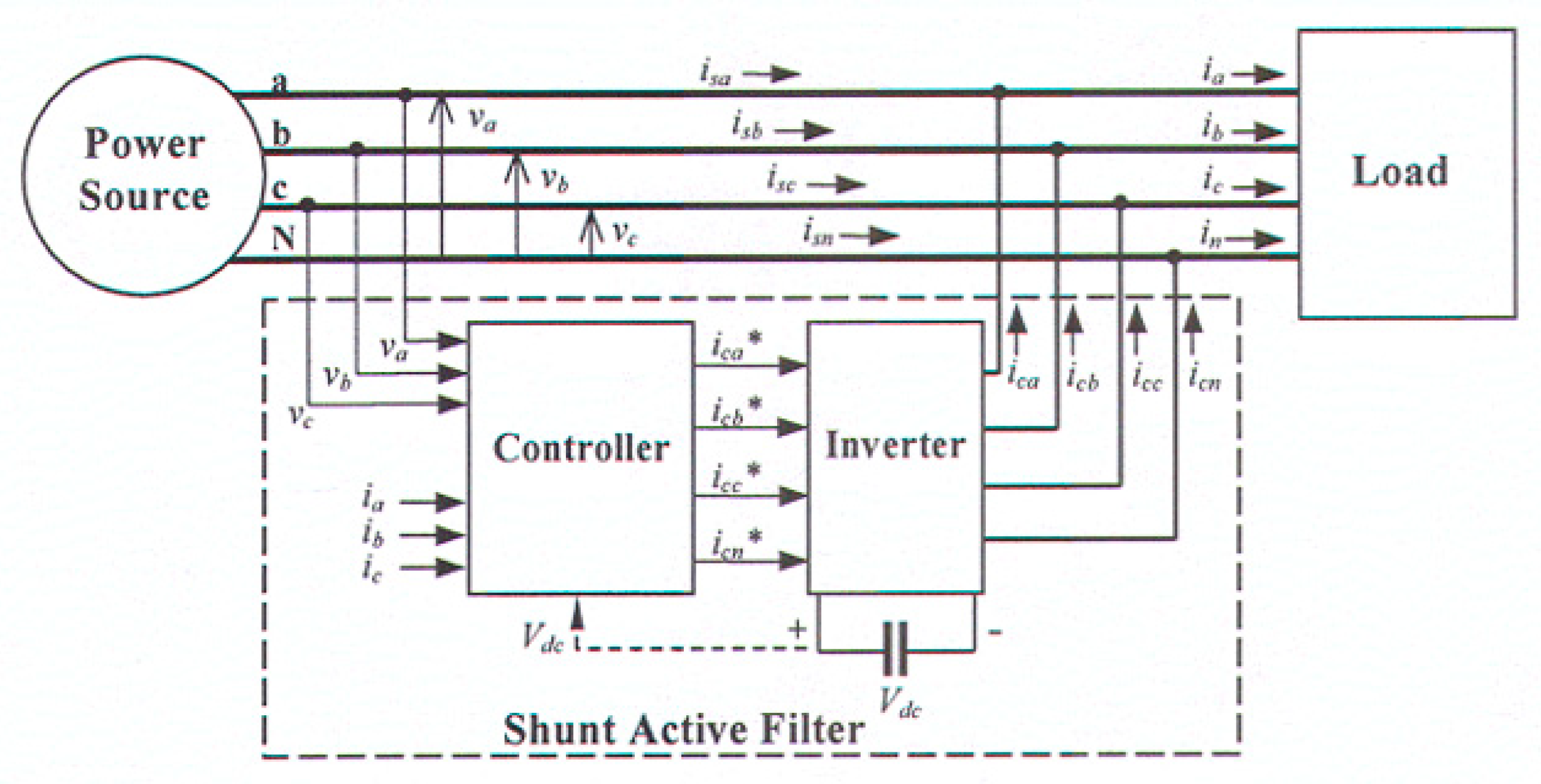
Figure 1 depicts an electric schema for a shunt active filter placed in a three-phase supplying system with null wire, designed for current harmonics compensation and load balancing, aiming to remove the current through the null wire [
33].
The power stage is mainly a voltage source invertor, with a single capacitor (CDC) on the D.C. link (the filter has no internal supplying source). Through control, CDC acts like a current source. The controller uses as inputs the phase voltages (
) and load currents (
) and computes the reference currents (
) which should be used by the inverter to produce the compensation currents (
) [
33].
This solution requires 6 current transducers and 4 voltage transducers and the inverter has 4 terminals (8 switches for the power semiconductors).
For balanced loads without current harmonic orders multiple of 3, there is no need for compensation along the null wire. A single 3-terminal inverter with only 4 current transducers is required and fewer computations have to be done by the controller [
31].
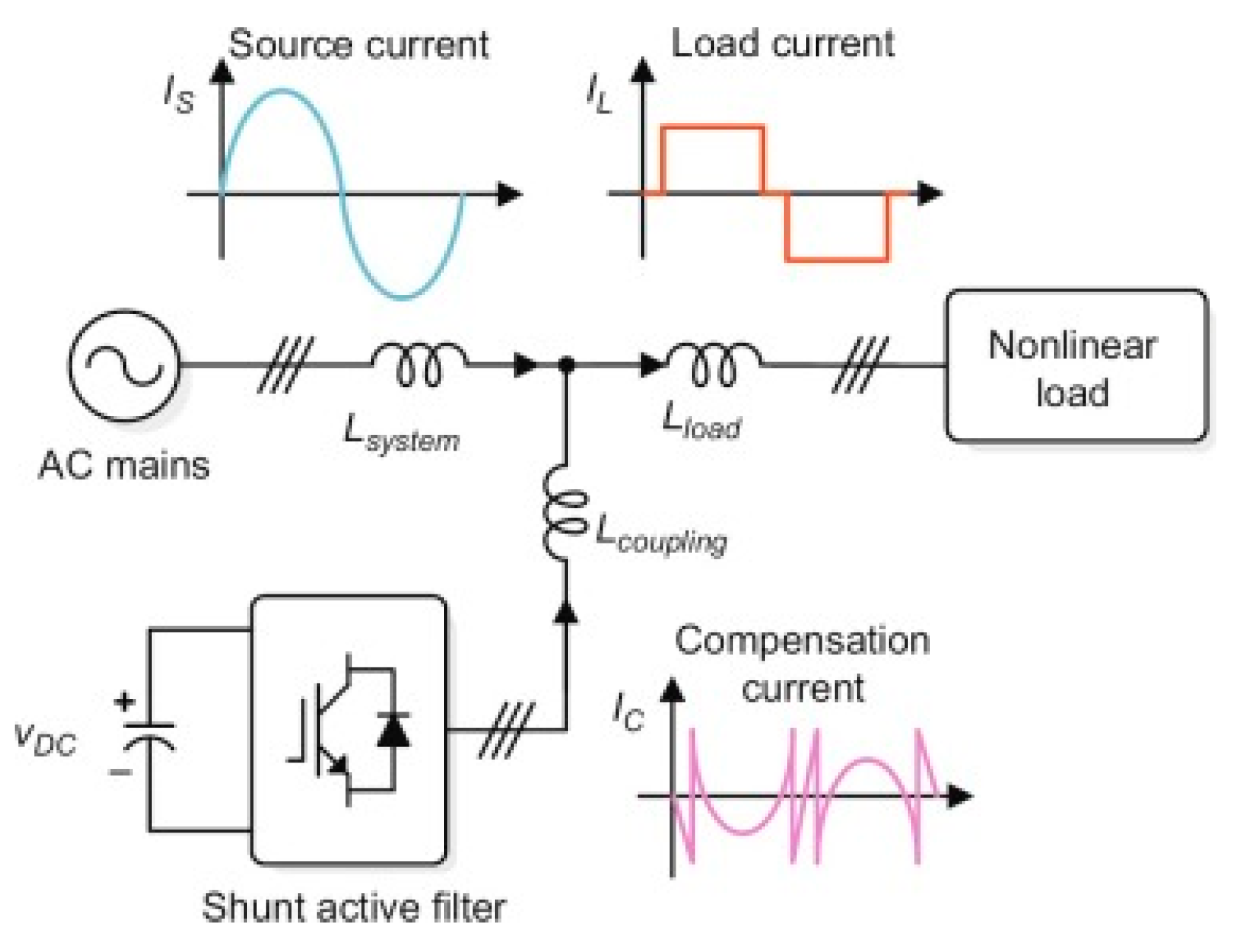
Shunt active power filters compensate current harmonics by injecting equal but opposite harmonic compensating current. In this case, the shunt active power filter operates as a current source injecting the harmonic components generated by the load but phase- shifted by 180 degrees. As a result, components of harmonic currents contained in the load current are canceled by the effect of the active filter, and the source current remains sinusoidal and in-phase with the respective phase-to-neutral voltage [
33]. This principle is applicable to any type of load considered as a harmonic source. In this way, the power distribution system sees the nonlinear load and the active power filter as an ideal resistor. The compensation characteristics of the shunt active power filter in an ideal case are shown in
Figure 2 [
33].
The power’s components
p and
q are written after transposing voltages and currents into the
frame as follows [
16,
20]:
The
p-
q theory belongs to an entire class of methods which can be used for the active filters control and has the following characteristics [
33]:
- −
It is intrinsically a theory for three-phase systems;
- −
It can be applied for three-phase, symmetrical or non-symmetrical systems, if the voltages and/or currents contain higher harmonics;
- −
It relies on instantaneous values and allows for an excellent dynamic response;
- −
It involves simple computations (actually only algebraic expressions which can be implemented using different processors);
- −
It allows some control strategies (e.g., instant constant supplied energy or sinusoidal current).
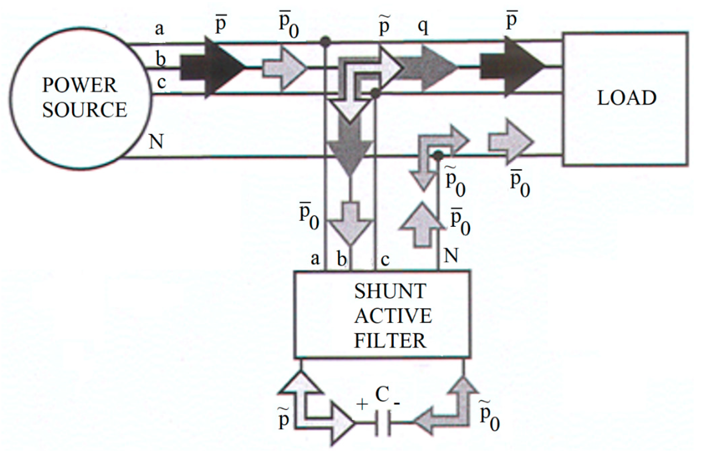
The principle of compensation of power components in this case is depicted by
Figure 3 [
30].
In order to compute the reference currents for compensation in the
coordinates, one has to use Equation (9) and the compensated powers (
and
q) [
33]:
As long as the homopolar current has to be compensated, the homopolar compensated reference current is equal to
i0:
In order to obtain the reference-compensated current using the coordinates
a,
b,
c, the reversed transformation is applied to Equation (10) [
33]:
where [
30]:
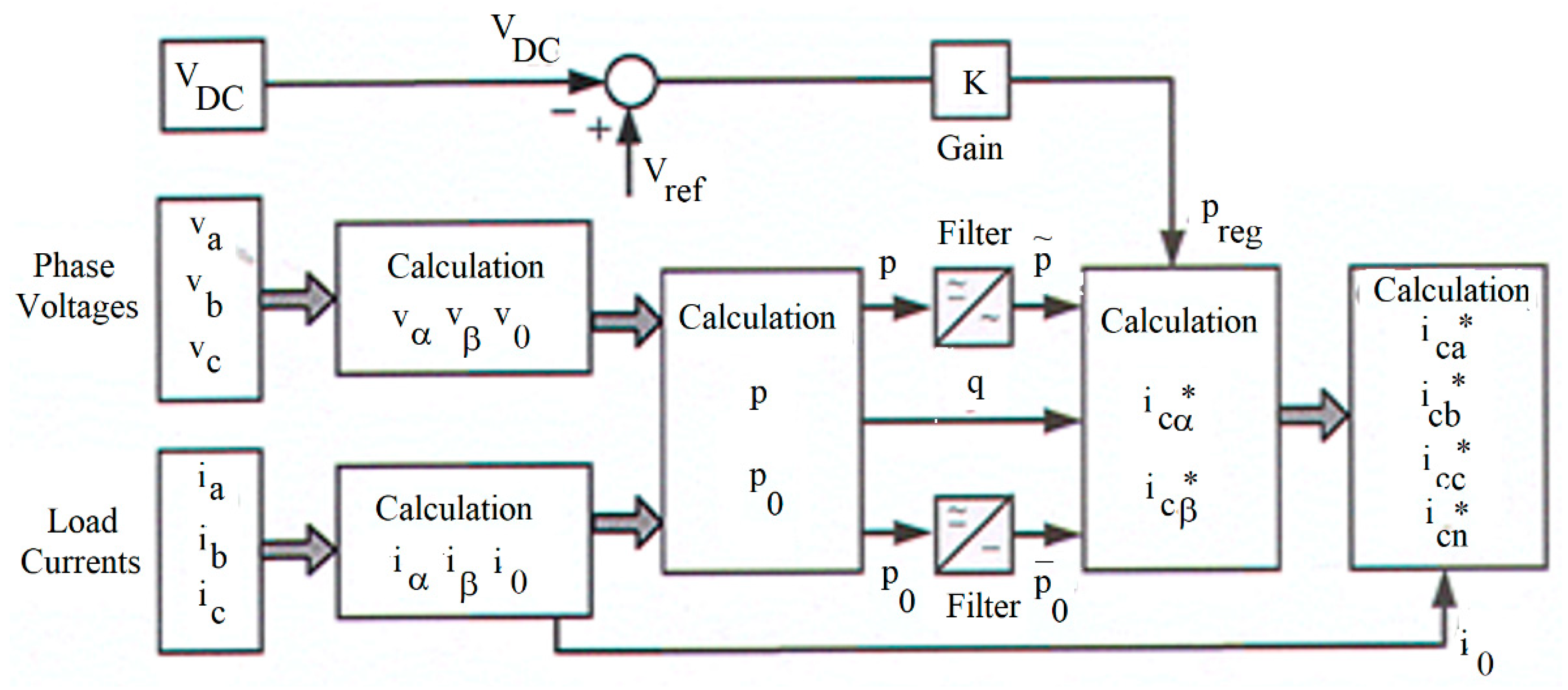
The equations from this subsection are depicted by
Figure 4 and are valid for a control strategy of a shunt active filter for a constant instantaneous power source [
33].
When applied to a three-phase system with sinusoidal symmetrical voltages, the following results are obtained [
33]:
- -
The phase currents from the source become sinusoidal, symmetrical (for an ideal case) and in-phase with the voltages (in other words, the power source “sees” the load as being purely resistive and balanced);
- -
The current through the null wire is forced to zero (even the current harmonics of order 3 are compensated in an ideal case);
- -
The total instantaneous supplied power will be in this case:
Active filters are up-to-date solutions to PQ problems. Shunt active filters allow the compensation of current harmonics and non-symmetries for superior harmonics, together with power factor correction, and can be a much better solution than the conventional approach (such as capacitors for power factor correction and passive filters to compensate for current harmonics) [
33].
The implementation of active filters based on the
p-
q theory are cost-effective solutions, allowing the use of a large number of low-power active filters in the same facility, close to every problematic load (or group of loads), avoiding the flow of current harmonics, reactive currents, and neutral currents through the facility power lines [
33].
Despite all these, the
p-
q theory can evaluate only the current harmonics after compensations. It is unable to evaluate neither the non-symmetry of voltages (which will automatically be decreased after the compensation of the higher current harmonics) [
2], nor the power factor for the fundamental harmonic or after reducing the harmonic weights. Moreover, it cannot evaluate which is the sequence of steps for compensation accomplishing. At theoretic level, one can demonstrate that firstly one has to diminish the current harmonics with an active filter and, afterward, one should improve the power factor considering the rest of harmonics!
2.2. Powers Definition Based on Separation in Active, Reactive, Distorting Powers
The definitions issued by the Romanian C-tin Budeanu in 1927 for reactive and fictitious powers [
11] were used by I.S. Antoniu and M. Gafencu [
12,
13]. They issued a generalization of the single-phase power definitions [
12,
13], considering the (re)active powers as being bi-linear forms [
31]. This theory is named Antoniu–Gafencu theory.
The harmonic decompositions made possible a subsequent determination of (re)active powers for distorting regime by Antoniu and Gafencu [
12]. Using tensors, one can determine relations to define the active, reactive, and distorting powers at balanced or unbalanced three-phase systems which operate in distorting regimes. For a balanced nonlinear load, the voltages and currents can be decomposed as [
12]:
The three-phase systems defined by Equations (15) and (16) allow a vector representation in the linear vector space of the trigonometric polynomials [
12]:
where:
Uj and
Ij (
j = l, 2, 3)—represent the vectors (first-order tensors) corresponding to the voltage and phase current with the vector space E;
represent the projections of the voltage’s vectors
Uj along the axis
Kx/y of a subspace
E1/2 of the odd/even functions. Similar equations can be used for currents.
Based on these observations, using the tensor method, one can deduce the powers for a balanced three-phase network which operates in a distorting regime [
12]. Using the scalar products of the voltage and current vectors for each phase and considering the vectors’ orthogonality condition, one can determine the powers described below [
12]:
(where
represent the phase active powers), or:
- (ii)
Reactive power
The phase reactive powers can be obtained using the scalar products between voltages and current, previously shifted by π/2 (by multiplying with
β):
or:
- (iii)
Distorting power
The distorting power can be expressed with:
Its absolute value can be computed with:
Equation (26) represents the general form of the total distorting power of a three-phase system operating in a distorting regime and is not influenced by the neutral point origin [
12].
Obviously, considering Equations (21), (23), and (29), one can say that the total apparent power of a three-phase system is lower than the sum of phases’ apparent powers (
). [
12]. Therefore, the following relation can be written as [
12]:
The total power factor expresses the relationship between the active power under ideal operation conditions and
S [
12,
31]:
where
represents the active power of all phases.
With this theory, one can define the (re)active, distorting and apparent powers by using the separation of power components according to the Antoniu–Gafencu theory for single-phase systems [
31].
Despite Equation (26), one can evaluate the total distorting power as the sum of the phase distorting powers. Experience proved that the results yielded by Equations (19) and (20) are close to the sum
. As a consequence, one can determine the total apparent power with
and evaluate the power factor with Equation (28) [
31].
The results yielded by Equations (21), (23), and (26) provide modalities for measuring, charging, compensation, and correct definition of some PQ indices before and after compensation, from both technical [
31] and economic points of view.
The distorting power diminishing actually assumes the diminishing of harmonic power components from voltages and currents with different harmonic orders. This process is followed by a diminishing of high harmonic components from the spectrum of (re)active powers [
31].
3. The Schema Used for Testing a Shunt Active Filter
In general, the active filters are developed based on a technology which uses inverters (usually voltage source), employing the Pulse Width Modulation (PWM) of the output voltage [
24]. The active filters can be classified considering criteria such as [
24]: (a) the nature of the compensated current (D.C. versus A.C. filter); (b) the objectives to be reached (active filters installed by individual consumers in order to satisfy their own compensation-related requirements—placed near one or several loads generating identifiable harmonics or active filters installed in substations by owners of low or medium voltage electric networks and/or by distribution feeders), and (c) the configuration of the filtering system.
Considering the configuration and the modality to connect the active filter, Shunt (Parallel) active filters (PAF) remove and/or diminish the harmonic currents [
2], preventing them from penetrating the supplying system. Various topologies (e.g., Dual Parallel Topology or Three-Level Inverter) were conceived [
29,
30].
The PAF compensates the current harmonics by injecting some compensation currents equal in absolute values but opposite to the harmonic currents. PAF is controlled such as to absorb a compensation current from the utility in order to cancel the current harmonics on the A.C. side (e.g., a rectifier with thyristors or a PWM rectifier with a D.C. link capacitor for traction systems). The parallel active filter cannot damp the harmonic resonance between a passive filter and the supplying source impedance [
24].
In order to provide the possibility to check the behavior of a PAF and to make some observations related to its power related efficiency, tests with a filter of this type were made on a test stand.
The initial structure of the modernized trams did not include choppers for the supplying voltage regulation. The authors improved this solution by implementing choppers in the supplying circuit of each tram. Data recorded over 6 months revealed that the supplying technique which included choppers resulted into energy savings of 47% (power electronics was used to improve the drive). The trams’ drive was initially made with 150 kW D.C. motors (300 V D.C.)—each tram was equipped with 2 pairs of motors, one per axle. One chopper per axle was used for acceleration whilst a single chopper was used for regenerative braking (the recovered energy was meant to be sent back to the tram’s supplying network in order to be consumed providing that other trams were simultaneously connected to the same supplying line).
The adopted solution did not solve the problem of power efficiency from the point of view of the society operating the trams. Tests accomplished in the transformation stations revealed that the use of choppers did not reduce the non-sinusoidal regime occurring as a consequence of supplying the tram lines from the secondary winding of certain 20 kV/380 V A.C. transformers, through power rectifiers with diodes which supply a 750 V voltage to the D.C. line.
Therefore, the next step was to improve the power consumption efficiency by compensating the unpleasant effects in the stations used to transform the energy at medium/low voltage.
In order to check the proposed solution’s power efficiency and to evaluate the efficiency of the parallel active shunt, a series of tests were accomplished on a test stand (
Figure 5).
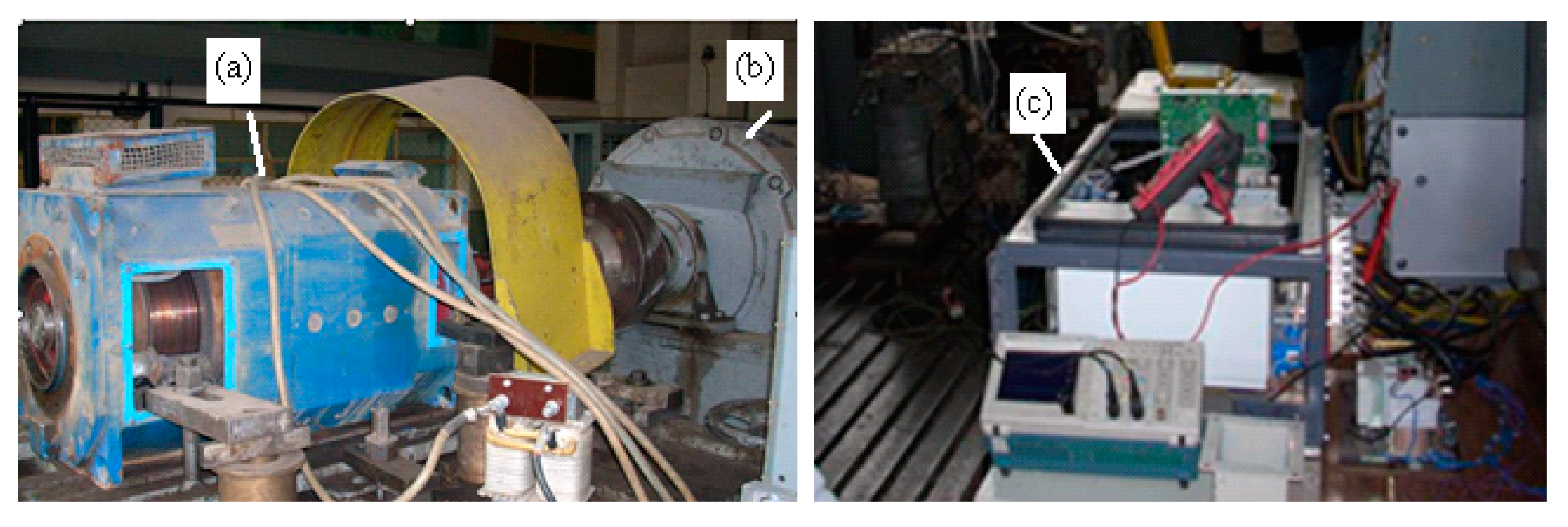
A D.C. motor (
Figure 6a), and a chopper (
Figure 6c) were tested in a schematic with regenerative braking. An asynchronous generator was used for the recovered energy (
Figure 6b).
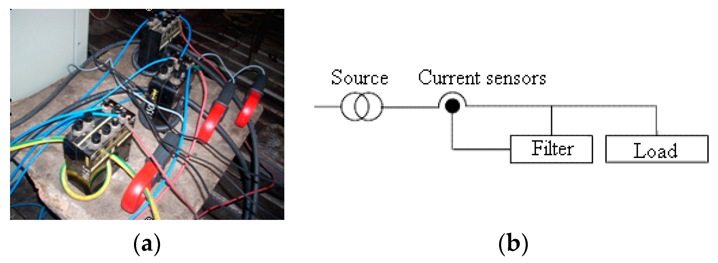
Dedicated data acquisition systems (DAS) were used to measure the currents and voltages from the secondary winding of the transformer (
Figure 7). The currents through filter are acquired by means of current test transformers of high precision (class 0.1) (
Figure 8).
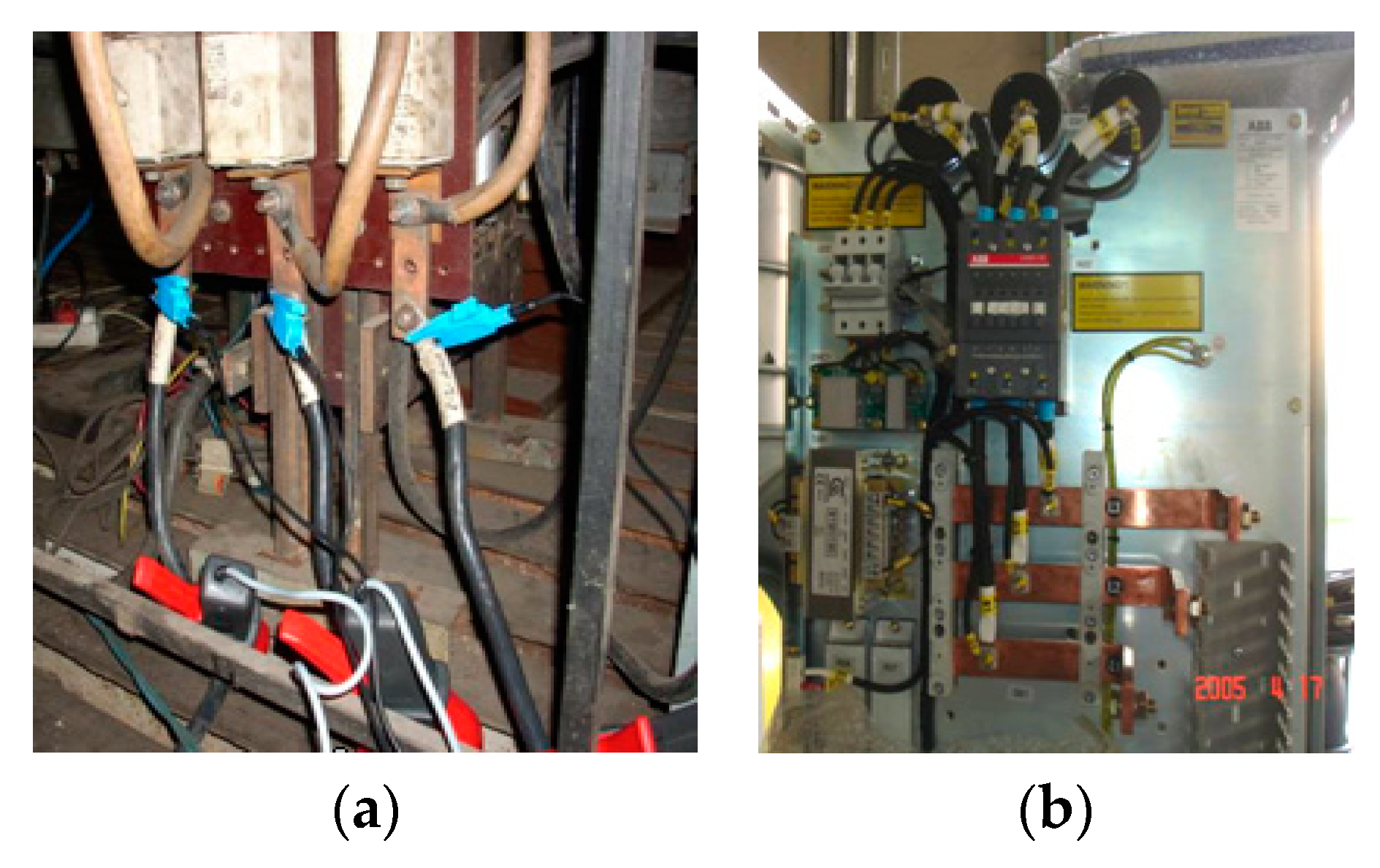
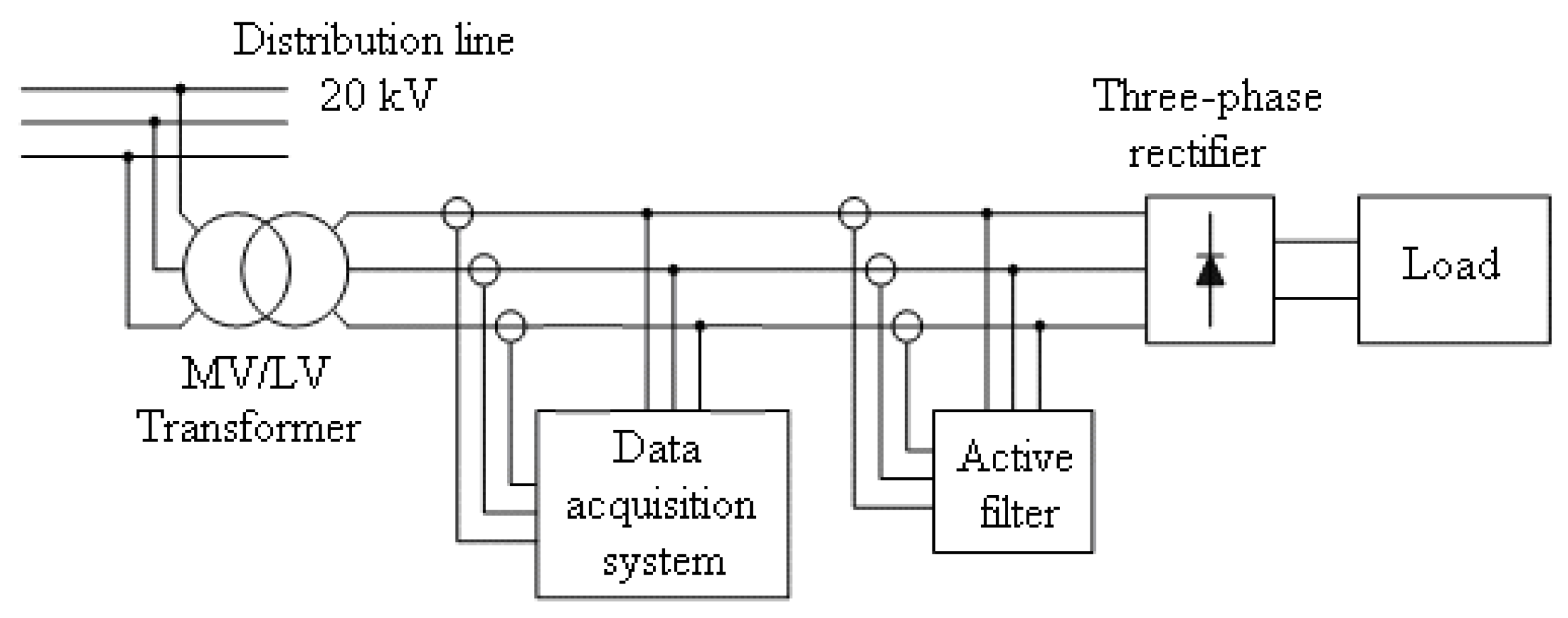
As depicted by the schematic in
Figure 9, the tested circuit contained: a D.C. motor of 150 kW (DCM), supplied by a 930/750 V D.C. step-down chopper, an active filter and a 20 kV/380 V A.C. step-down transformer that supplies a three-phase rectifier with diodes (the employed data acquisition systems (DASs) were not depicted in
Figure 9). During the regenerative braking regime, DCM delivers power in the supplying network.
4. Active Filter Behavior
4.1. Study of Active Filtering in the Permanent Regime of a Traction Motor for Urban Vehicles, Supplied from a Chopper
The tested load consisted in a three-phase rectifier with diodes, chopper, DCM, and asynchronous generator. The analysis was concerned with various powers in the absence/presence of active filtering. Three cases were considered, with or without the active filtering, as follows:
- −
Case α: the D.C. motor was supplied with a power of around 70% from its rated power;
- −
Case β: the D.C. motor was supplied with a power of around 91% from its rated power;
- −
Case γ: the D.C. motor was supplied at its rated power.
The three-phase voltages and currents from the secondary winding of the 20 kV/380 V transformer were acquired with a DAS designed and realized for this application, for each of the analyzed cases. The acquired data were transferred through a serial interface to a PC, where they were processed with dedicated software, based on FFT (developed by authors).
Details are presented below for the case γ, both for a direct supply from the secondary winding of the 20 kV/380 V transformer (without compensation) and, respectively, when the load was supplied after the connection of the active filter.
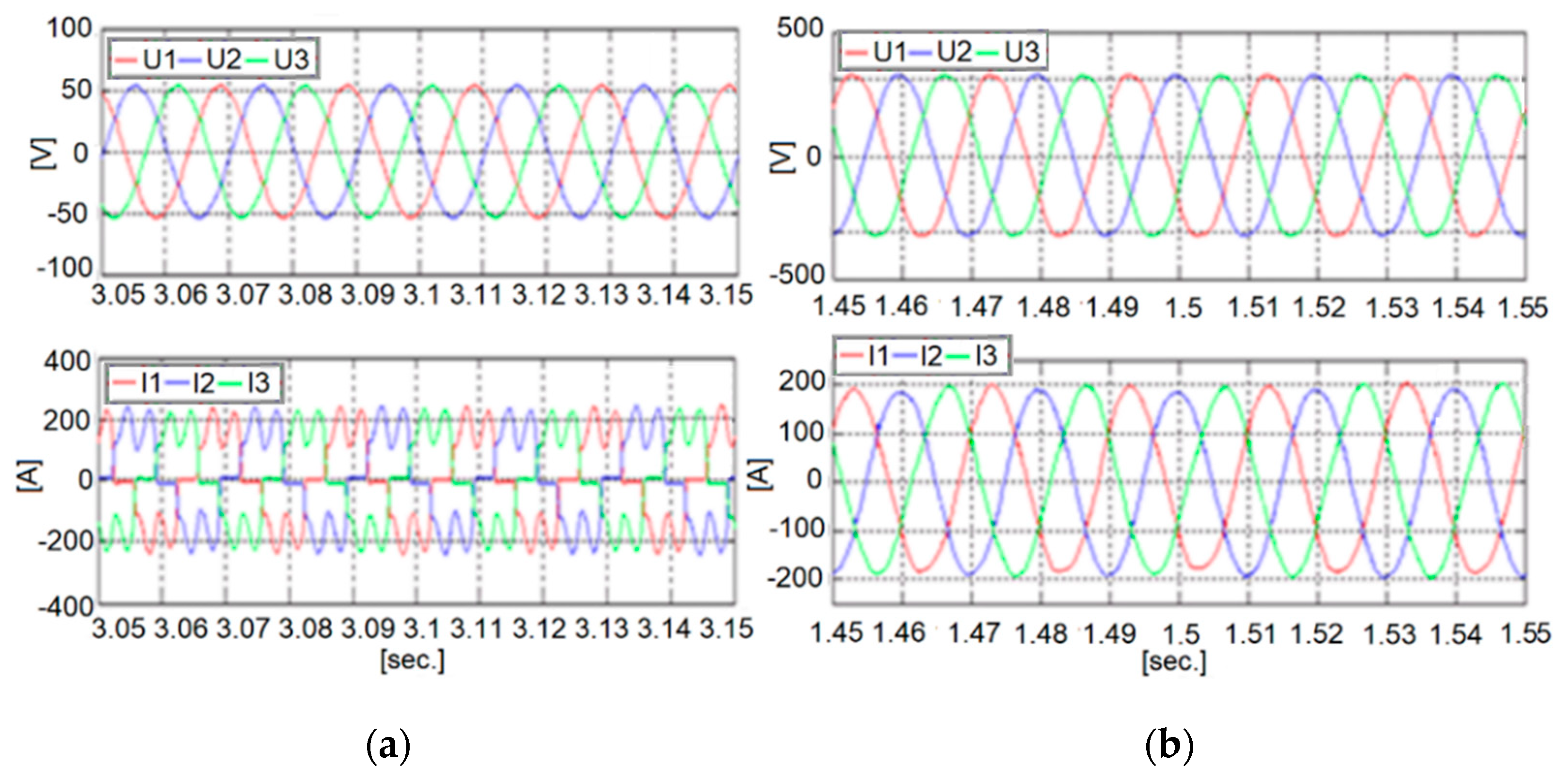
Figure 10 shows the electrical waveforms recorded during the operating regime without compensation and, respectively, without the least significant 49 harmonic orders—due to compensation with the active filter (depending on the setting of the active filter).
Original programs were used to determine the harmonic components: the magnitudes, initial phases, and weights (relative to the fundamental harmonic). The first 25 most significant harmonics of the voltages and absorbed currents are gathered in
Table 1 and
Table 2 (when no compensation was made), and in
Table 3 and
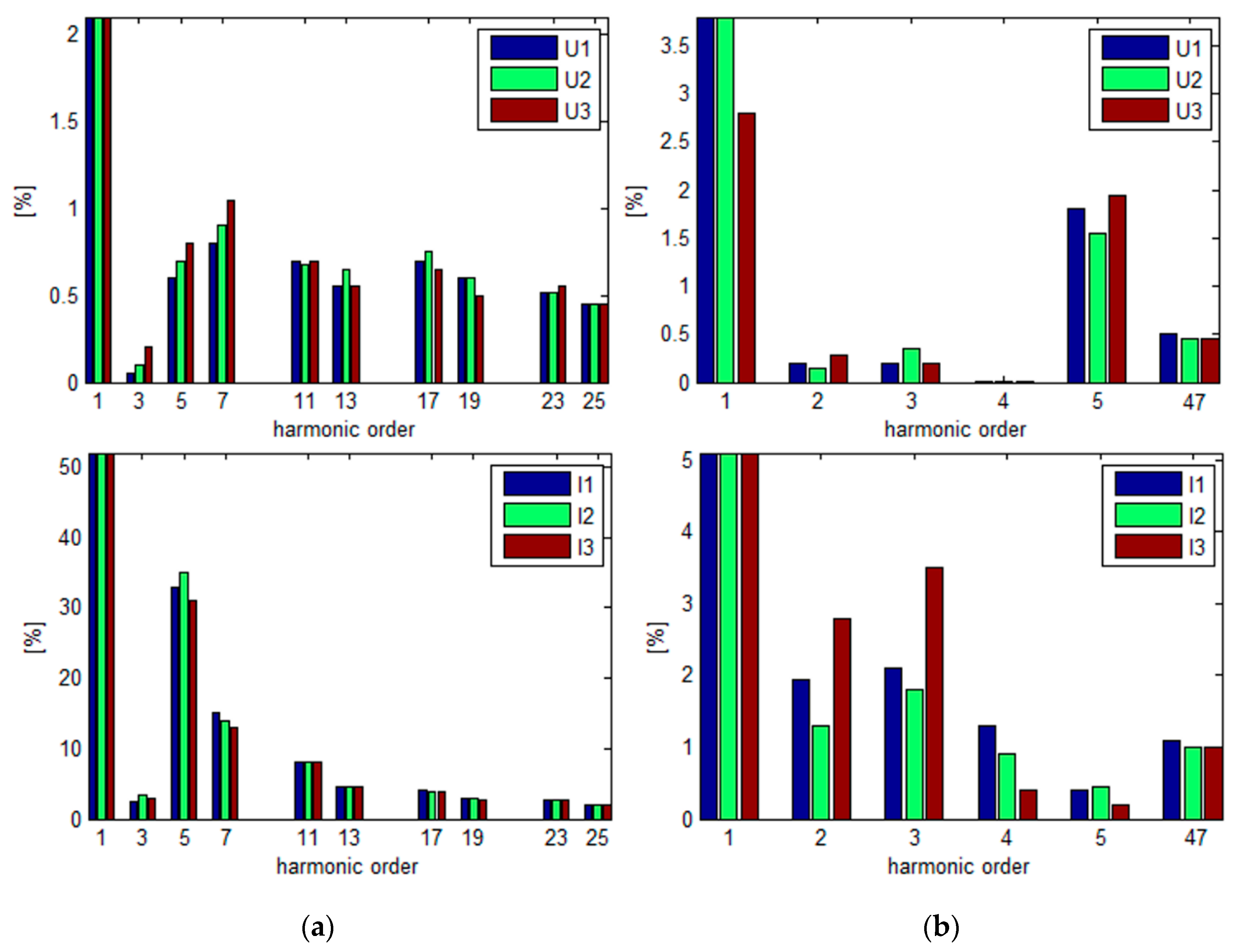
Table 4, respectively (when filtering was made). The harmonic content for both cases are depicted by
Figure 11a,b. The RMS values for phase voltages and absorbed currents, fundamental harmonic of phase voltages, and absorbed currents, as well as certain PQ indices (peak factor and total harmonic distortions) are gathered in
Table 5 for the α, β, and γ cases.
In order to evaluate the power efficiency when using active filtering, quantities such as the active power—(AP), reactive power (RP), distorting power (DP), apparent power (APP), and the power quality factor were also determined.
Equations (20)–(28) were used, because they allow for the determination of apparent power and power factor. Unlike the theory of instantaneous powers, the standard IEEE 1459-2010 might have had been used too, yielding similar conclusions.
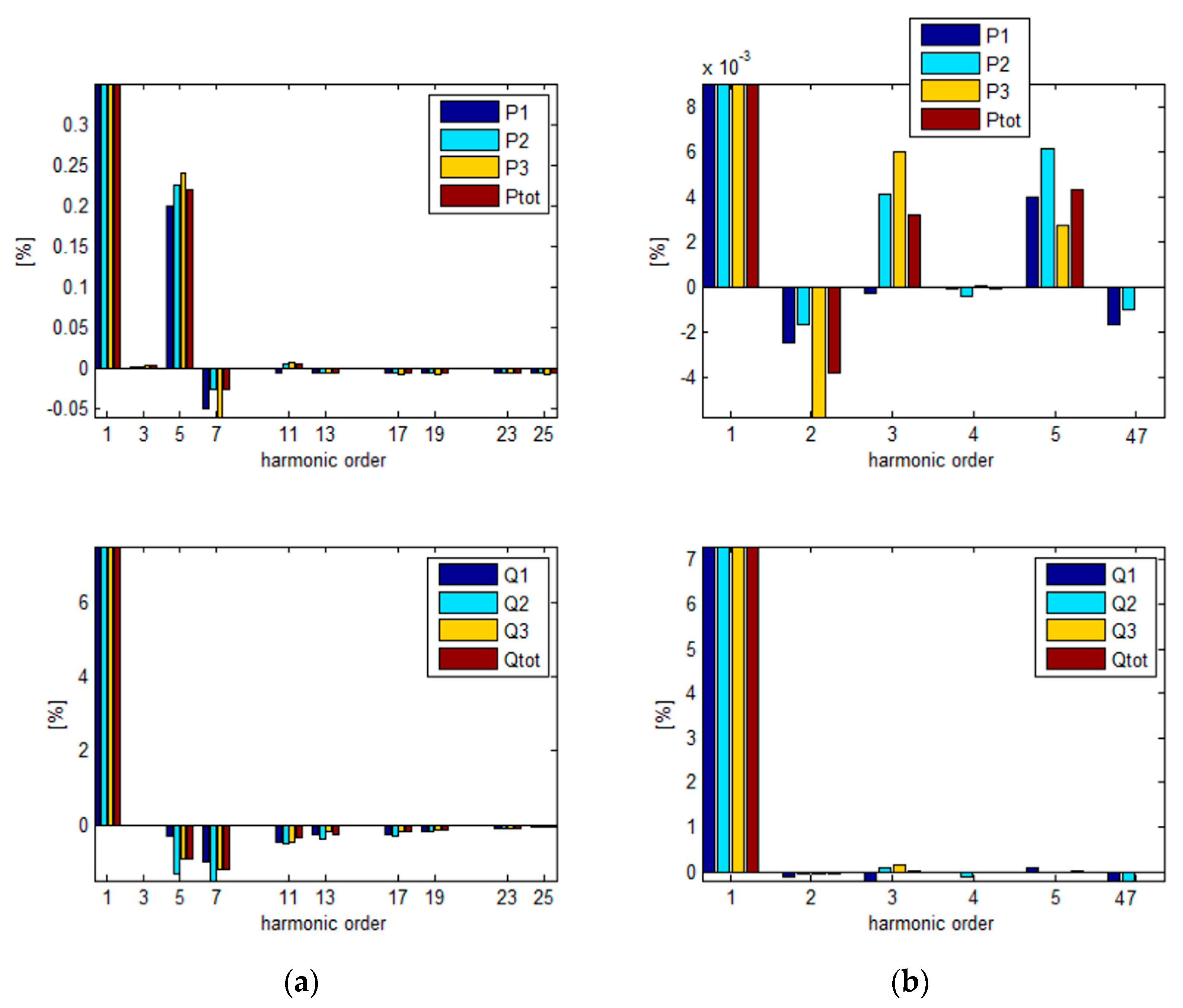
Any of the two approaches concerned with powers determination leads to similar conclusions, differences appearing for powers corresponding to high harmonic orders. Yet, similar conclusions could be drawn relative to the power factor. The spectral components of the phase powers absorbed from the supplying source are depicted in
Figure 12 for the RPs and APs, before and after compensation. The power components are gathered in
Table 6 for all cases (α, β, and γ).
4.2. Study of Active Filtering in a Transient Regime of a Traction Motor for Urban Vehicles, Supplied from a Chopper
The shunt active filter efficiency can be evaluated using the reaction of the driving system at transient regimes, other than those associated to fault regimes [
2].
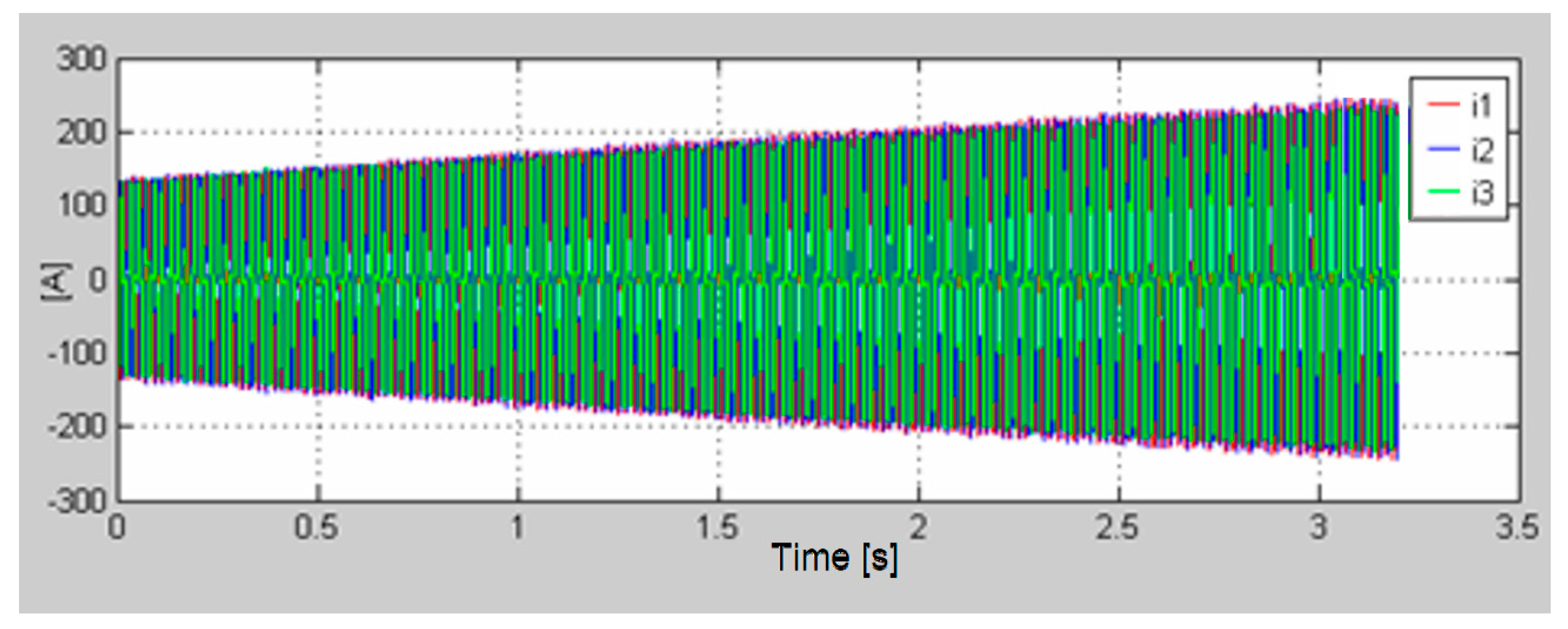
Figure 13 depicts the currents absorbed from the supplying network for the worst case (connecting the load during the start of the driving system).
Data acquired at different moments were analyzed and it was proved that the active filtering was efficient as long as during this transient regime the harmonic currents were below the limits prescribed by IEEE Standard 519 [
2].
5. Active Filter Efficiency Evaluation from Technical Point of View
Another conclusion yielded by the harmonic analysis addressed the diminishing of the HDs of currents absorbed by the load such as they were lower than the limits imposed through the IEEE 519-2914 standard [
5].
For the evaluation of the full load compensation, one has to notice that the load’s power factor (as seen from the source) is around 0.9 (value imposed for the neutral power factor).
The analysis concerning the filter’s efficiency revealed that:
- I.
For identical RMSs of currents absorbed from the source, the total APPs are almost identical, but lower APs (used for the driving system) are lower when the filter is not connected;
- (a)
An AP of 137.71 kW was obtained with the filter disconnected, whilst the filtering resulted into an AP of 147.7 kW (case β);
- (b)
An AP of 149.7 kW was obtained with the filter disconnected, whilst the filtering resulted into an AP of 160.6 kW (case γ).
It means that the useful active power required by the load is the same in both cases from the case I (b), but different active powers absorbed are obtained:
- -
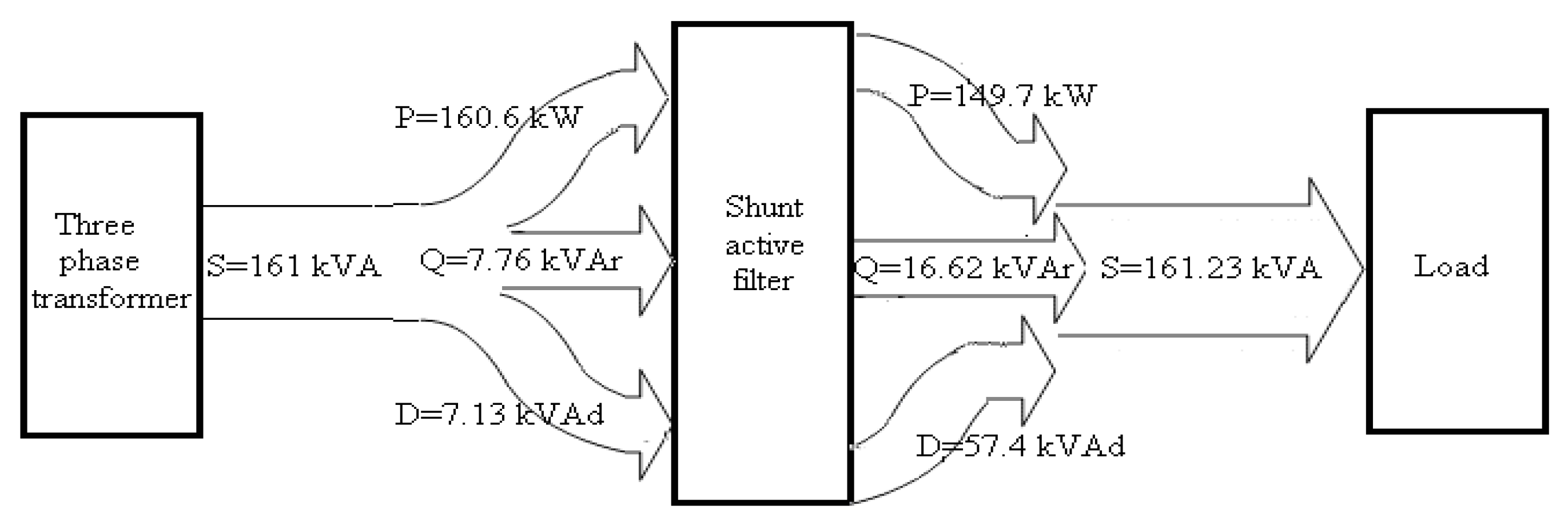
When the load is directly supplied from the transformer’s secondary winding, the total apparent power was equal to 161.23 kVA for rated power, but due to the non-sinusoidal regime, it was divided into: active power (P = 149.7 kW), reactive power (Q = 16.62 kVAr) and, respectively, distorting power (D = 57.4 kVAd). The load induced the non-sinusoidal regime, which affects both the supplying source and the D.C. motor.
- -
The use of a shunt active filter resulted into: identical total apparent power absorbed from the source (S = 161 kVA), increased active power absorbed from the source (P = 160.6 kW) and, respectively, significant diminishing of the reactive and distorting powers (Q = 7.76 kVAr; D = 7.13 kVAd).
This happens because the filter absorbs a quantity of active power higher than that required by the load and reconverts a part of it in additional reactive and distorting powers required by the load. A diagram of power flows is depicted by
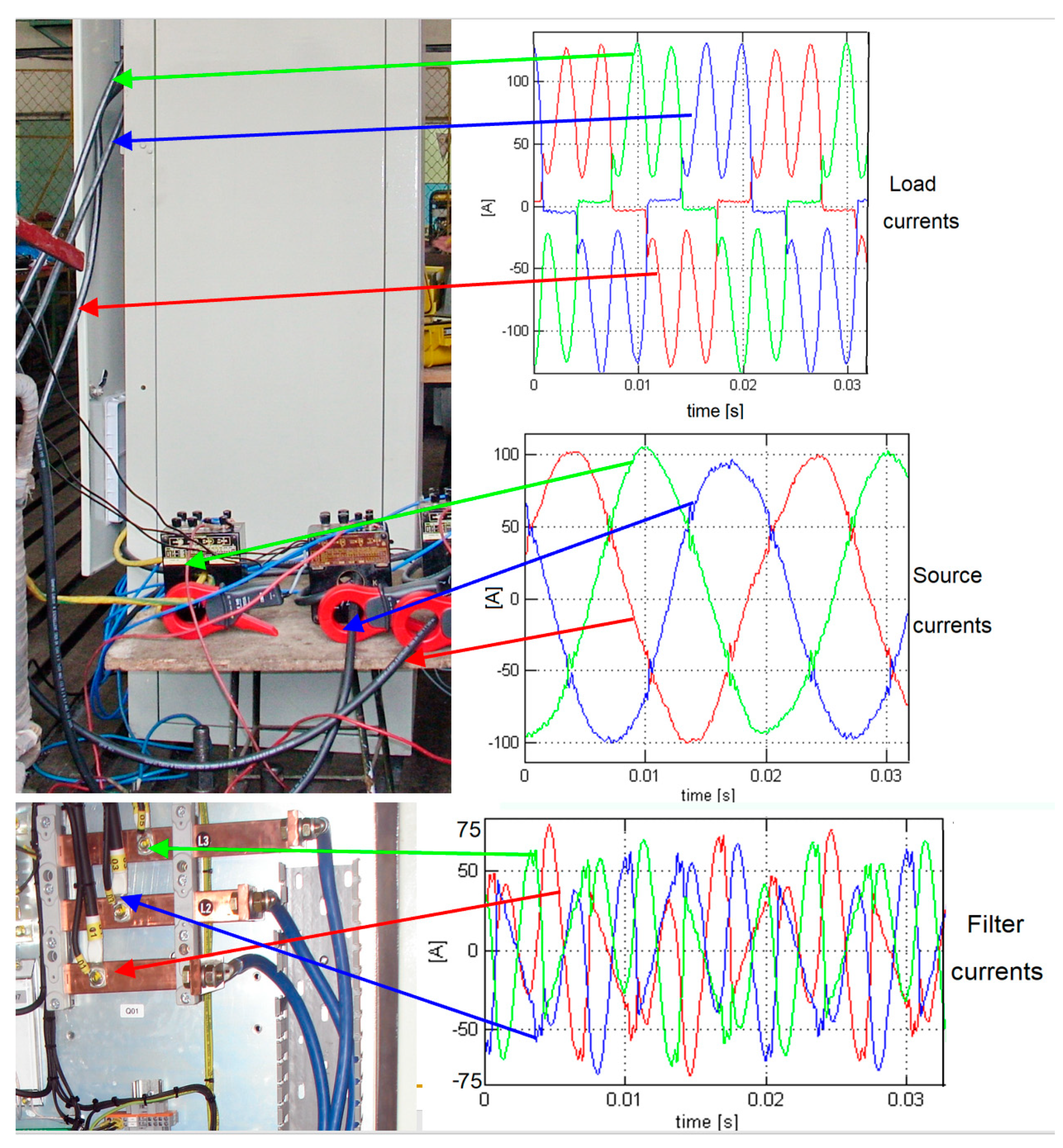
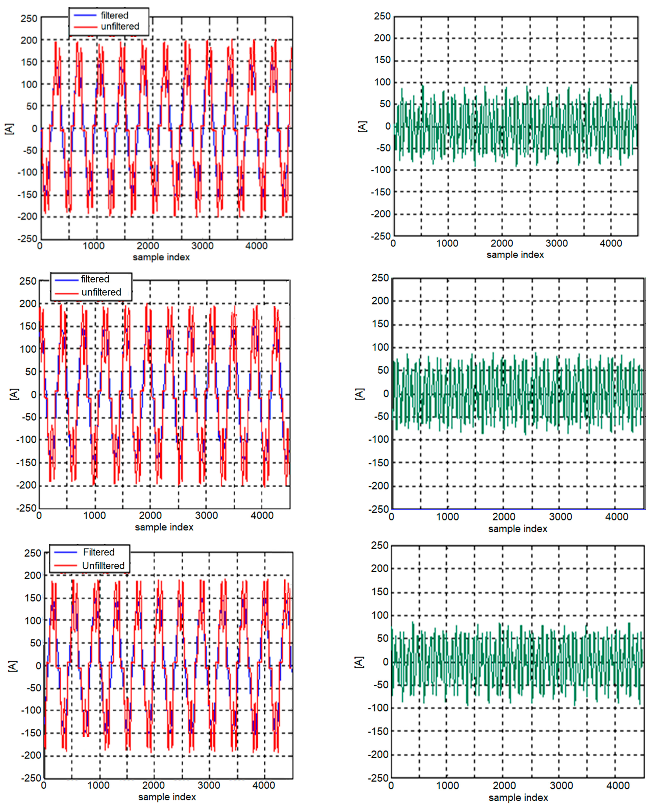
Figure 14 and the values before and after compensation, as well as the currents through filter for a single-phase RMS value of 100 A can be seen in
Figure 15.
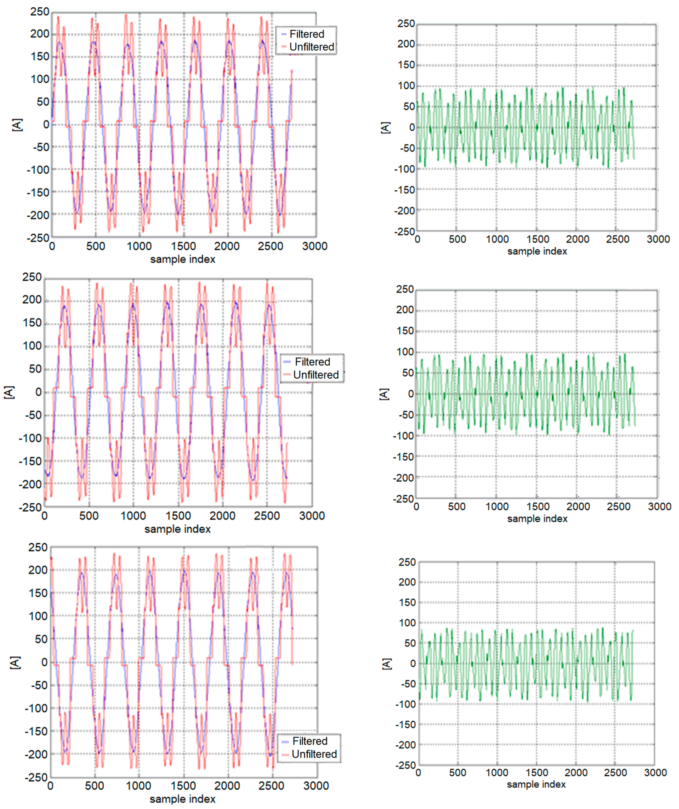
Figure 16 represents the values before and after compensation, as well as the currents through filter for an RMS value of 132 A per phase [
2].
Figure 17 represents the values before and after compensation, as well as the currents through the filter for a single-phase RMS value equal to 142 A.
- II.
The filtering effect was also studied for a different AP absorbed from the source (around 149 kW). When the filter was disconnected, the APP absorbed power was S = 161.23 kVA (case γ) whilst the filtering process resulted into a smaller value (148.08 kVA—case β). Possible explanations for this are given below: (a) When the load is directly supplied from the source, the absorbed current from it is higher; it has an RMS value of almost 142 A per phase and this reveals a significant distortion relative to the supplying source, considering that the counterpart RMS value of the fundamental harmonic is around 132 A. (b) When the load is supplied from the source by means of the shunt active filter, the current absorbed by it is almost sinusoidal, with a single-phase RMS value of around 132, which is very close to that for the fundamental harmonic.
The results presented above prove that the filtering efficiency can be underestimated if it is computed considering the energetic point of view. On the other hand, if it is associated to the fundamental harmonics’ RMS values, the same driving efficiency is obtained, but with an additional consumption of APP in the case when filtering is not provided.
The analysis concerning the filter’s efficiency are summarized in
Table 7, based on the above conclusions (for all α, β, γ cases).
At the same time, for a certain RMS value associated with the fundamental harmonic, the total current harmonics flowing through the load are obviously higher in the case without filtering, as revealed by the currents’ HDs. The use of active filtering results in a diminishing of current harmonics relative to the supplying network. In this way, the impact of harmonic currents over other consumers connected to the supplying network is diminished (the supplying voltages’ distortion does not exceed the limits imposed by the standards).
6. Active Filter Efficiency Evaluation from Financial Point of View
The load keeps on being supplied by non-sinusoidal currents and negative effects are noticed. Therefore, as in the case of nonlinear loads, an analysis from the point of view of power efficiency must be done. For this aim, we proposed to define several factors (coefficients), as follows:
This factor should be considered when evaluating the efficiency of compensation and the ROI for a certain solution selected in order to obtain a full compensation of the load. A value of 7.75% was computed for the analyzed case.
- 2.
A relative coefficient (), related to the additional active power absorbed from the source, which should be used for compensation:
For the cases analyzed in
Section 5,
= 7.28%.
This coefficient is mainly useful for users who intend to install active filters. They will be aware on the additional charge paid for not obeying the limits of the power factor (at least 0.9 for the neutral power factor) and, respectively, for the harmonic currents introduced in the network. They will also be able to determine the economic efficiency of installing the active filter by comparing both coefficients, as explained in the examples below:
- I.
Determining and using CS
The accomplished apparent power saving is determined by the computed difference. This involves, after compensation, an effective apparent power consumptions equal to 148.08 kVA.
From an economical point of view, at a continuous operation within a year, one obtains the following total consumption of apparent power (equivalent to apparent energy):
For an approximate price of 100 Euros/MVAh, tests allowed for an evaluation of saving as follows:
For an estimated price of the filter (including accessories) equal to 100,000.00 Euros, the ROI will be approximated to:
(In this case, we did not consider different categories for the savings of active power and, respectively, of reactive power—charged as 10% from the total active power.)
- II.
Determining and using CP
- II.1.
The use of active filter results in a saving of reactive energy. The difference between the reactive energy before and after compensation has to be computed at the beginning:
For one year, one obtains:
In terms of active power gained, one obtains the following difference (after and before compensation):
In Romania, the consumer is charged for reactive power considering it to be 10% from the consumed active power. Under these conditions, the active energy gain for one year is:
Considering an estimated price for active energy equal to 100 Euros/MWh, the reactive energy price will be equal to 10 Euros/MVAr.
It comes out that the total price of the recovered energy is:
For an estimated price of the filter (including accessories) equal to 100,000.00 Euros, the ROI will be approximated to:
- II.2.
ROI is difficult to estimate due to particularities in national laws.
Therefore, if one uses the coefficient
CP, it comes out that for an active power equal to 160.6 kW, after the filter’s plugging, one obtains a recovering rate equal to:
Considering an active energy price equal to 100 Euros/MWh, one obtains an annual consumption of recovered active energy as follows:
The cost savings due to the active filter are estimated as:
In this case, the ROI will be:
This calculation method yields more accurate results as compared to the case when the prices of recovered active energy and, respectively, of recovered reactive energy are calculated individually (ROI21 and ROI22).
As a consequence, both coefficients defined above (CS and CP) provide useful information with respect to the financial aspects when implementing an active filter for an industrial consumer.
The values of both coefficients reveal similar values for the ROI in both situations (by comparing ROI1 and, respectively, ROI22 from Equations (34) and (44))!
One has to mention that the theory of instantaneous powers does not allow for the evaluation of financial effects induced by the active filter plug-in. A correct estimation of these effects requires definitions for certain power components which should be used for the computation of APs, RPs, DPs, and APPs, along with the power factor.
Therefore, in practice, one has to:
- (a)
Make a technical evaluation of the active filter influence by using either the theory of instantaneous powers or the 2-nd theory, relying on the definitions for APs, RPs, DPs and APPs and power factor, respectively. However, one has to take into account that the theory of instantaneous powers can only be used for the technical solution implementation, including the active filter control;
- (b)
Make a financial evaluation of the active filter influence by using the theory that relies on the definitions for APs, RPs, DPs, and APPs and power factor, respectively, making use of the additional coefficients defined by Equations (29) and (30).
7. Conclusions
The full load compensation for the analyzed cases relies on the following assumptions: (a) the diminishing of harmonic currents absorbed from the supplying source, irrespective of the nature of the driving regime, such as to be lower than the limits imposed by IEEE 519-2014; (b) compensation of the power factor associated with the fundamental harmonic such as to exceed the neutral value [
2]. Therefore, the settings of PAF have to be made in the following sequence: firstly, the harmonic distortion reduction and afterward the compensation of the power factor for the fundamental harmonic.
The current harmonic distortion for the uncompensated load was quite large, not complying with the IEEE 519-2014 Standard. The lower was the current absorbed by the load, the higher was the absorbed current harmonic distortion (as it may be noticed in
Table 5 for the cases α, β, and γ). However, the supply voltage harmonic distortion was greater with the increase of the currents absorbed by the load (see
Table 5—cases α, β, and γ).
Basically, the absorbed current’s magnitudes are influencing the supplying voltages distortion, and not vice versa.
The installation of the shunt active power filter is significantly improving the operating mode of the PSN, but with additional active power consumption from the source.
Therefore, in order to determine the energy efficiency for the proposed solution at the load terminals, two quantities (coefficients) must be introduced (Equations (29) and (30)). They are intended to allow the users of such loads to decide over the solution of improving the energy/PQ, technically and economically. New definitions for new compensation factors are proposed. These are required for full load compensation. Based on the definitions from Equations (29) and (30) and the results yielded by numerical processing, we obtained ROIs around 9.5 years (ROI1 = 9.49 years, ROI22 = 9.76 years). The specialty literature does not provide economical evaluations concerned with the improvement of energy efficiency based on load compensation.
Another technical question which requests an answer is: has an individual compensation of the distorting loads to be performed, or can one use a “per group” load compensation? Both technical and financial calculations and estimations should be used when making such decisions!
The current waveforms from the active filter (
Figure 15,
Figure 16 and
Figure 17) reveal the need for measures to diminish the EMIs which might appear between the filters and the supplying network.
The installation of the shunt active power filter is neither protecting the load nor a part of it (the D.C. motor in this case), against the non-sinusoidal currents owing to the three-phase diode rectifier [
34,
35]. Therefore, for protecting the load in these cases, different protection measures are necessary, with associated costs. Otherwise, the life span of the D.C. motor would dramatically decrease and a series of other load’s components may be subjected to a negative influence.
In this paper, the theory of Antoniu–Gafencu for the non-sinusoidal regime in three-phase circuits was used [
12]. Similar results were obtained with the theory presented in the IEEE 1459-2010 Standard [
4,
5] (for example, the total apparent power determined for the case γ—unfiltered case, was S = 161.230 kVA when Equation (11) was used, whilst when using Equation (13) from the standard IEEE 1459-2010, we obtained S = 161.198 kVA). The distorting and reactive powers for high-order harmonics (appearing in Equations (9) and (11)) correspond to the power components presented in the Standard IEEE 1459-2010 for the non-fundamental effective apparent power. The compensation analyzed in the paper was intended to diminish the reactive and distorting powers. The reactive power absorbed from the source was reduced, whilst the distorting power was reduced through the diminishing of the current distortion (obeying the Standard IEEE 519-2014 [
6]). This is equivalent to the approaching (under the reserve of possible errors) of the power factor (corresponding to the voltage and current fundamental harmonics). The “p-q” theory does not provide the full load compensation, because compensation along the fundamental harmonic cannot be defined [
28]. Basically, the p-q theory is useful for compensating the non-sinusoidal and/or unbalanced regimes, but not for the compensation of the fundamental harmonic (neither a power factor nor a global apparent power can be defined in the p-q theory) [
34,
36].
Another element that can be used to evaluate the filter’s efficiency is the filter’s reaction to transients. For the analyzed cases, the behavior was correct, the transients did not reveal any negative influence over the operation of the entire system (source + filter + load).
Our future work takes as starting point the observation that most of the known compensation solutions (involving passive, active or hybrid filtering, respectively, waveform modelling in various shapes) rely on different implementations of the Fourier transform. Such solutions require many technical restrictions, due to the accuracy of harmonic decompositions, which is acceptable only for low harmonic orders (usually those mentioned in the standards in force for the quality of energy/power). New approaches are required with respect to the decomposition of waveforms whose harmonic spectra include high frequencies. Among them, a special role is played by decompositions based on Wavelet Transforms.
In the same time, new standards should be conceived in order to make a difference between the specific features of energy/power quality and those of Electromagnetic Compatibility at low frequencies (lower than 150 kHz). For the time being, many technical limits affect the accurate measuring equipment for the frequency range 2–150 kHz.
Another issue is related to the accurate extraction of components associated to electromagnetic interferences frequencies (noise) from the signals which also include low frequency components belonging to the domain of the quality of energy/power. Solutions for this technique were conceived by authors in two recent studies [
37,
38].


