Adaptation of Users to Future Climate Conditions in Naturally Ventilated Historic Buildings: Effects on Indoor Comfort

Abstract

User behaviour can significantly affect indoor thermal comfort conditions, as well as energy consumption, especially in existing buildings with high thermal masses where natural cross ventilation is the main strategy to reduce cooling loads. The aims of this paper were: (i) to compare how behavioural changes evaluated by means of rule-based and stochastic models lead to changes in indoor thermal comfort levels, and (ii) to define the patterns of indoor thermal comfort in historic residential buildings in future scenarios. To this end, a historic building located in Molfetta (Southern Italy) was analysed using a dynamic energy simulation engine in five weather scenarios (Typical Meteorological Year, current extreme weather file 2018, predicted weather files for 2020, 2050, and 2080 generated by morphing method), and stochastic and rule-based models for window openings were adopted and compared. The results showed that the stochastic model was more accurate than the rule-based one, resulting in a reduction of discomfort conditions during the summer period between 30% and 50% in all climate scenarios. However, although the differences between predicted discomfort levels using rule-based and stochastic models tended to increase, discomfort levels still appeared to be not acceptable in the 2050 and 2080 scenarios due to the rising temperature driven by climate change.

1. Introduction

The global climate is changing. The average temperature of our planet is changing. According to an analysis conducted by NASA, the temperature has increased by 1.1 °C since 1880, and the cause is largely attributable to the increasingly higher levels in the atmosphere of carbon dioxide (CO₂) and other greenhouse gases produced by human activities [1]. Unfortunately, the rise of temperature is intended to increase, and with the global warming of 1.5 °C, the risks associated with climate change for natural and human systems are higher than ever, as reported by the Intergovernmental Panel for Climate Change (IPCC) in the Special Report on Global Warming [1]. According to Pagliano et al. [2], to be able to apply strategies that fight these global climate changes, however, we need to act locally. For this reason, it is interesting to analyse the changes taking place in the Mediterranean region that, according to the Research Institute for Development [3], appears to be one of the most sensitive regions in the world to climate change. This sensitivity is due both to the localisation of the region in a transition zone between two different climates (temperate in the middle latitudes and arid in the North African area) and to its specific geographical characteristics. The European Union has defined the prevention of the danger of climate change as a priority, defining directives aimed at reducing energy consumption, increasing energy efficiency, and, at the same time, reducing greenhouse gas emissions [4]. To meet the set objectives, however, it is appropriate to significantly increase the energy performance of new buildings, but at the same time, it is necessary to recover and improve the existing building stock. Existing buildings are much more sensitive than new buildings to climate change [5] and are, especially in Italy, in greater numbers than new buildings.

Although not specifically mentioned by the European policies, among existing buildings, historic ones undoubtedly deserve significant attention. Indeed, the renovation of such buildings requires a balance between several criteria, including not only energy consumption reduction, but also the needs of the building fabric, users, as well as economics, and climate change-related factors [6]. Nevertheless, while research on material and technical measures is widely discussed [7], there is a lack of literature concerning the user behaviour in the management of historic buildings, which can significantly affect the energy demand [8]. Likewise, the potential impacts of climate change on occupants’ thermal comfort, HVAC systems, and the energy performance of historic buildings still appear to be understudied, requiring further research to be conducted [6].

This work was intended as a contribution to fill these research gaps, since its main aim was to assess the potential impact of climate change on a historic building in terms of indoor comfort, taking user behaviour into account. Unlike the majority of studies, thermal comfort was evaluated by implementing a stochastic behavioural model of occupants, allowing the uncertainty related to user behaviour to be included in the analyses.

In detail, two objectives were pursued: (i) comparing how behavioural changes evaluated by means of rule-based and stochastic models lead to changes in the regime of indoor operative temperatures; (ii) defining the patterns of indoor thermal comfort in historic residential buildings in future years by using a stochastic model. A simple workflow summarizing the study conceptual framework is given in Figure 1.

1.1. Future Climate Projections and Modelling

Unlike the weather forecast, it is not possible to make certain, deterministic predictions of how the climate will change in the next century and beyond since climate change projections are affected by uncertainties. In order to overcome the problem of uncertainties, it is possible to use models that define certain output values obtained through very specific assumptions related to future forcing scenarios. These scenarios are the so-called Representative Concentration Pathways (RCPs) and were introduced by the IPCC in 2004. There were four scenarios obtained that predict the increasing quantities of greenhouse gas and CO₂ emissions (RCP2.6, RCP4.5, RCP6, and RCP8.5) and were named after the likely values of radiative forcing in 2100 (2.6, 4.5, 6, and 8.5 W/m², respectively) [9]. These scenarios were used as boundary conditions for the Global Circulation Models (GCM). The outputs obtained from a GCM cannot be directly used for Building Performance Simulation (BPS) analyses because they have a monthly temporal scale and a spatial resolution in the range of 100–300 km². In order to make the GCM outputs usable with the BPS tools, they must be scaled to the correct spatial and temporal resolution [10]. There are several approaches to perform this scaling, namely dynamical downscaling, statistical downscaling, and hybrid downscaling.

In dynamic downscaling, regional or local climate information is derived from the Regional Climate Model (RCM). RCMs, similar to GCMs, are numerical models that require pre-established boundary conditions derived from GCMs. RCMs require great computational power to be developed and require a lot of storage space in order to create the data sets. Statistical downscaling, on the other hand, is based on the determination of climate data using rule-based or stochastic approaches. This approach is simpler than dynamic downscaling, in relation to the fact that there is a greater amount of hourly data that can be directly extracted from the RCMs. The morphing method, developed by Belcher et al. [11], is part of the statistical approach, which consists of three transformation algorithms applied to the hourly values of the climatic variables to be transformed. The three algorithms are the shift, the stretch, and the combination of shift and stretch. In some cases, when there is a need to reduce computational resources and the space to store data, it is possible to use hybrid downscaling. After obtaining the outputs from the various RCMs, these are scaled through statistical approaches.

1.2. Stochastic Modelling of User Behaviour within Buildings

As widely documented by the Annex 66 and 79 promoted by the Energy in Building and Communities programme of the International energy Agency (IEA-EBC) on the definition and simulation of occupant behaviour in buildings [12], the behaviour of the occupants is a key aspect for optimising the design of buildings and energy simulations. Having an in-depth knowledge of user behaviour and being able to quantify their impact with respect to building technologies allows researchers and professionals to develop simulations that are much more reliable and consistent with reality. Unfortunately, however, user behaviour is a very complex aspect to evaluate, above all because it is influenced by external factors—such as economics, culture, and climate—but also from internal ones, such as physiological or psychological ones. Precisely because of this complexity, there are many works in the literature that target user behaviour and analyse it in very different ways from each other. Generally, it is possible to use either rule-based models, stochastic models, or data-driven models. For further details, see [13,14]. Rule-based models are deductive models that are based on the presence of a predetermined set or rules or equations that associate an environmental parameter with an action. In this category, deterministic methods and schedules are included. Stochastic models are deductive models that trying to describe the behaviour of a system over time. These models are based on a group of random variables defined on a space of probability Ω and indicated by the parameter t, where t varies in index set T. Usually, the parameter t is called Time. In this way, the entire process is characterised by different results every time the analyses are run. These results are expressed in terms of the probability that a specific event happens according to the explanatory variables considered in the simulation. Four main and different models of adaptive behaviour can be identified.

(1)

Scheduled adaptive behaviour [15,16]: In the scheduled adaptive behaviour, a deterministic approach is used to associate an environmental variable with the action.

(2)

Bernoulli models [17,18]: Bernoulli models predict the probability of finding a building component (with which the occupants interact) in a given state. These models do not provide any information on the adaptive behaviour of the occupants, and it is preferable to use them to represent the energy consumption of a building rather than the indoor comfort conditions.

(3)

Discrete-time Markov models [19,20,21,22] describe the probability that a behaviour is adaptive to a changed condition in the next time interval. They can be developed based on both internal and external variables.

(4)

Discrete-event models [23,24,25]: Discrete-event models are Markov models that link an occupant’s action model to an external event.

Through regressions, it is possible to evaluate the weight of the occupant adaptive behaviour model by developing a certain number of parametric coefficients and making continuous distributions. The regression method is the most reliable for evaluating adaptive behaviour as it allows the evaluation of the probability of a certain event happening, again using explanatory variables. Finally, data-driven models are inductive models where the occupant behaviour is inferred from data collected in-field without using any explicit a priori knowledge on the phenomenon by applying statistical techniques. These include machine learning models and agent-based modelling.

1.3. Thermal Comfort Evaluation in Historic Buildings

In recent years, interest in historic buildings has increased as much as interest in climate change. It has been demonstrated how recovering and renovating buildings, bringing them to performance standards consistent with those provided for by the standard, is essential to increase sustainability and energy performance and to contrast the negative effects of climate change. In the work of Martinez et al. [26], residential, religious, and museum buildings, especially those belonging to the past two centuries, have often been the subject of study in Europe. Many of the studies are concentrated in Italy, which has a relevant share of historic buildings in Europe. Several studies are aimed at understanding thermal comfort conditions in traditional vernacular buildings. Cardinale et al. [27], through the use of building performance simulation, assessed the behaviour of Mediterranean vernacular architecture (Sassi constructions in Matera and Trulli construction in Alberobello), observing high levels of indoor thermal comfort despite the presence of external temperatures exceeding 35 °C. De Berardinis et al. [28] analysed the case of a masonry building in a small town in Abruzzo, assessing its energy behaviour following different technological solutions used to recover the building, while Balocco and Gazzini [29] evaluated, through a numerical analysis, different ventilation systems in historic buildings located in Palermo. Cantin et al. [30] assessed the thermal behaviour and thermal comfort of 11 historical dwellings in France, finding a very strong correlation between indoor and outdoor air temperatures. Ultimately, due to the low air tightness of windows and the high thermal transmittance of walls and roofs, historic buildings act as thermally open systems, whose performances are primarily affected by the outdoor environmental conditions.

Although several studies on indoor comfort in historic buildings have been performed, only a limited number of them include the effects of climate change. Recently, Hao et al. [31] reviewed the literature concerning the effects of global warming on historic buildings, focusing on different aspects such as energy performance and indoor comfort. As they pointed out, a lack of studies on indoor comfort in the future climate in historic buildings can be identified, since research tends to focus more on other topics, such as artifact preservation. An exception is given by [32], who analysed the overheating risk in a typical London dwelling, looking at: (i) four types of envelopes, including an unfilled cavity masonry; (ii) four window-operation scenarios; and (iii) two blind operation settings. Overheating risk was assessed in a bedroom during the occupied hours (night-time). Overheating was first evaluated according to TM52 for three categories (I, II, and III) and second according to a new index based on the duration where adaptive limits are continuously exceeded. Referring to the masonry construction, in the current climate, it did not show overheating problems, even under the worst conditions (window closed and no solar protection). On the contrary, overheating issues significantly increased due to the rising temperatures in 2030 and 2050 scenarios, with doubled values outside TM52 criteria. Even though blind use and window operations allowed the improvement of the overheating problems, Lee et al. pointed out that they cannot be enough to remove the issue, especially in the 2080 scenario. In a further work, Peacock et al. [33] assessed the potential impact of climate change on UK dwellings in terms of overheating based on two indices: the percentage of internal temperatures that exceed 28 °C during the occupant hours and the number of cooling nights in a year, assumed when the temperature of the bedroom at 11 pm exceeds 23.9 °C. They considered two weather scenarios (2005 and 2030) in London and Edinburgh cities, assessing the overheating risk for three construction typologies: a timber-frame dwelling, a twin leaf masonry dwelling with improved insulation, and a pre-1900 solid wall dwelling. They found that high thermal mass dwellings showed the lowest overheating, based on both the indicators. Despite this, the rising outdoor temperatures in 2030 still caused the increase of percentage of internal temperatures that exceed 28 °C, which ranged from 8–12% and from 1–2% in London and Edinburgh, respectively, as well as the number of cooling nights, which ranged from 27–49 and from 84–104, respectively. Escandón et al. [34] evaluated the impact of climate change in terms of adaptive thermal comfort, accounting for a building category that represented more than 40% of post-war residential stock. They pointed out an increase of the percentage of discomfort hours of about 36.6% in 2050.

As can be noticed, all these studies evaluated the energy behaviour and thermal comfort of buildings, but very few considered occupant behaviours. In this regard, one notable work is the one of Ben and Steemers [35], which dealt with the evaluation of the relationship between occupant behaviours in buildings (using a deterministic model) and energy retrofit strategies in existing buildings. The existing literature highlights that the issue of thermal comfort in buildings is of fundamental importance, especially where refurbishment works are needed. As fundamental as thermal comfort is, the behaviour of users—through their habits and the management of spaces and services—can significantly affect buildings’ energy consumptions. The deterministic model used in Ben and Steemers work [35] is a good starting point, but considered users’ presence statically, thus providing an inaccurate representation of the dynamic behaviour of the building.

As shown, studies evaluating climate change impacts on comfort in historical buildings appears to be limited, even more so considering occupant behaviour. The present work attempts to give a contribution to fill these research gaps, assessing thermal comfort in a historic building, both in current and future weather scenarios, by implementing a stochastic behavioural model of occupants. In this way, the uncertainty related to user behaviour has been included in the energy and thermal comfort assessments aiming at providing a more accurate description of the reality.

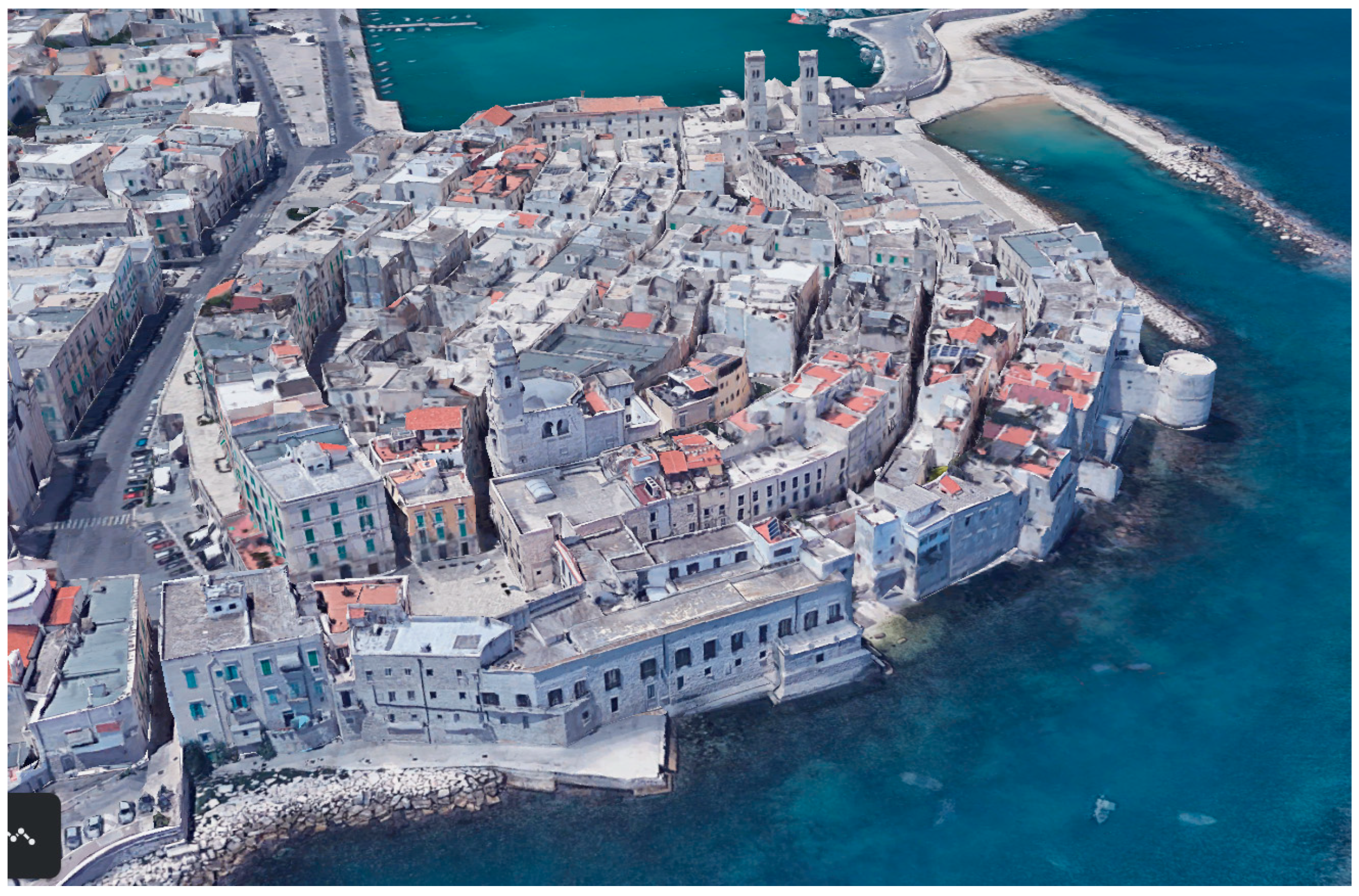
2. Case Study Selection and Monitoring Campaign

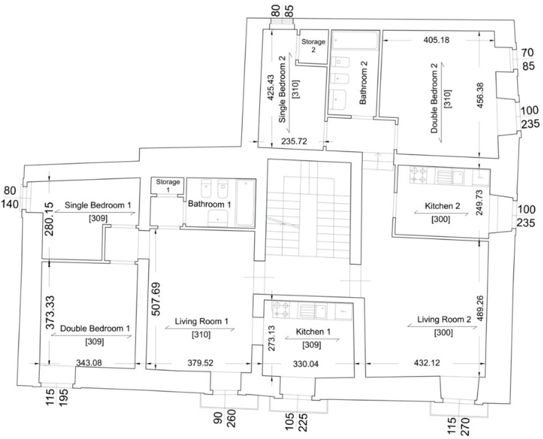
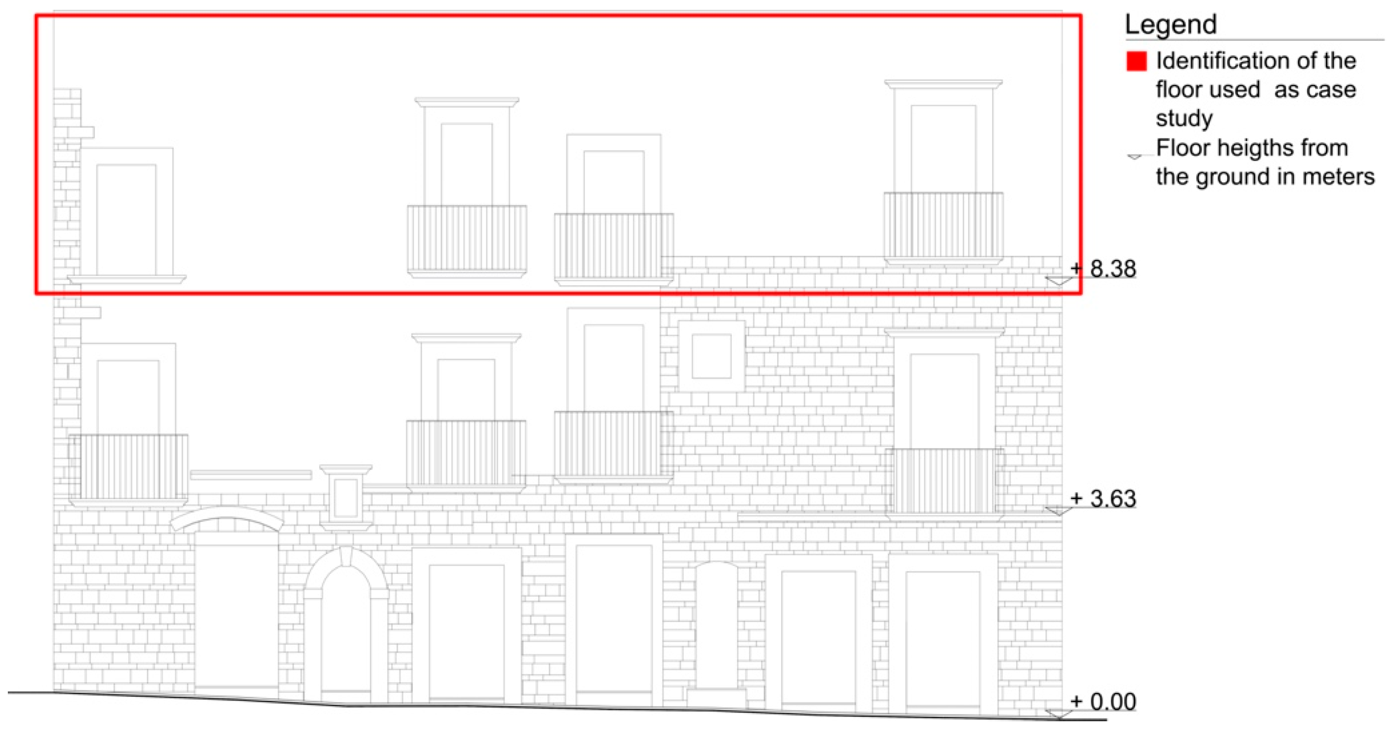
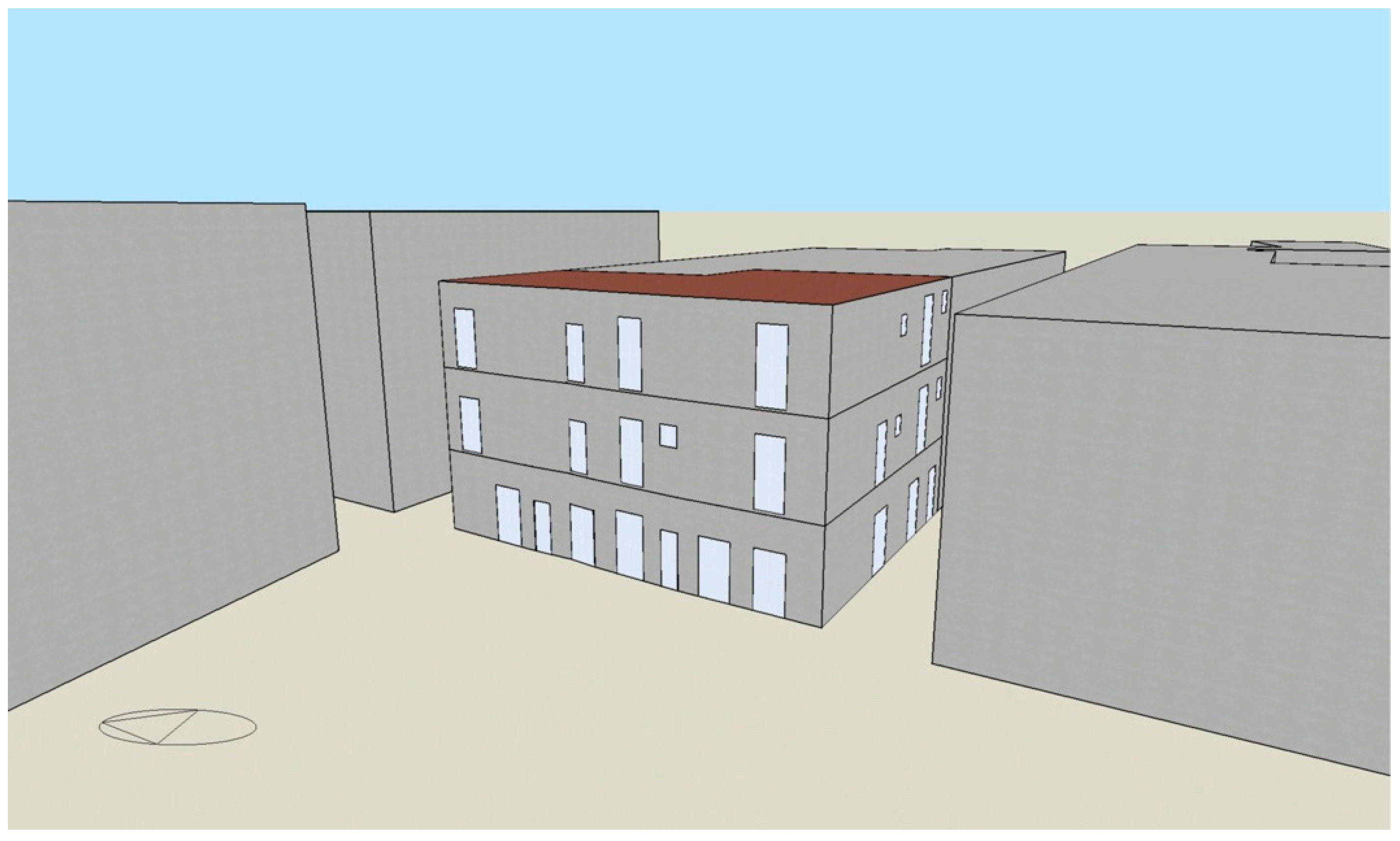
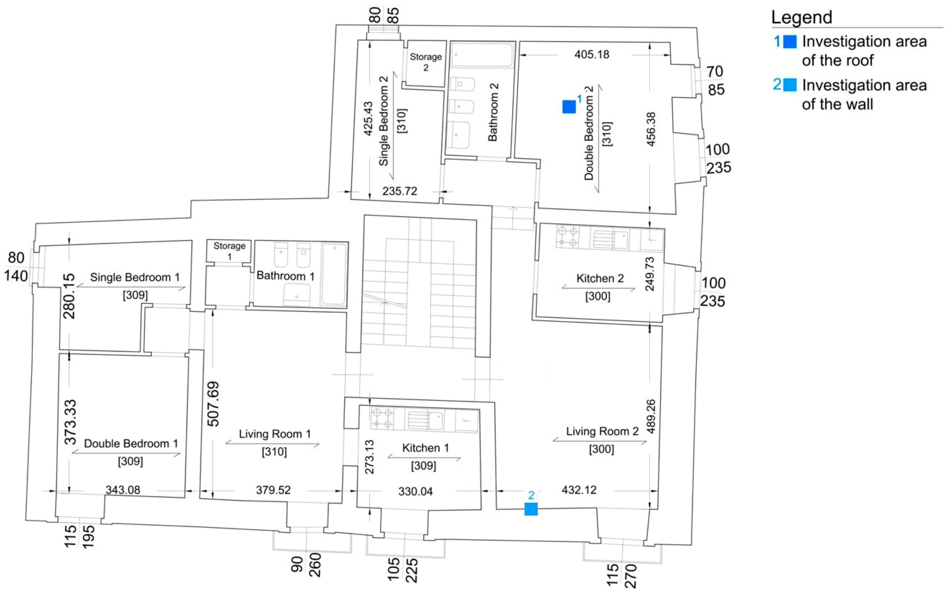
2.1. Case Study Selection

A representative case study that could mimic in a reliable way the behaviour of most of the historic residential buildings was selected. The building analysed is located in Molfetta (Apulia, Italy, 41°12′ N 16°36′ E). The city of Molfetta is characterised by typical south Mediterranean climatic conditions, is located along the coastline of the Adriatic Sea, and is included in the area Csa (hot-summer Mediterranean), according to the Köppen-Geiger climate classification. The building is located within the historic centre, which dates back to the Middle Ages and was developed until the nineteenth century. The historic centre consists of traditional buildings, mainly made of local stone masonry and wooden ceilings, and their arrangement follows a North/Northwest–South/Southeast orientation organised along quite narrow streets. In the historic centre, it is possible to find two recurring building typologies: the “tower-houses”, with narrow façades on the street—from 3 to 5 m wide—and prevalent internal development, and the “palace-houses”, with a large facade on the street and openings in every room. Both types are composed of up to five storeys, with the ground floor generally used as a small shop with an independent entrance and the upper floors arranged in apartments. The shops usually have stone barrel vaults, while the apartments have wooden ceilings.

The building selected was built in the 18th century and can be identified typologically as a “palace-house”. The building falls exactly into the type 1 category of UNI/TR 11552-2014 [36] regarding the construction type. Category 1 is the most common construction technology in most of the Italian regions for buildings built before 1950. From an analysis conducted by Fatiguso et al. [37], the building has typical characteristics such as the ones of all the other neighbouring structures located in the historic centre. The main characteristics of the building are:

-

Quite thin ceilings (about 18 cm depth), composed of wooden beams and decks and stone tiles.

-

Quite thick walls (thicknesses varying between 65–100 cm, following structural requirements), with two layers of square stone blocks and an internal cavity filled with mixtures of mortar and soil.

-

Narrow windows, generally not coeval with the building, with timber frames and double glazing.

-

Ground floor slab made of concrete and placed on a layer of stone and gravel blocks as a barrier against humidity.

Figure 2 and Figure 3 include, respectively, the typical floorplan and the main elevation of the selected building. The building is constituted of three floors. The ground floor was originally used as a shop, but now it has been reconverted into residential apartments, while the two upper floors host two apartments each. The building is located at the corner between two streets, with all the rooms adjacent to the principal streets, apart from the two single-use bedrooms, which are adjacent to the internal courtyard (see Figure 4).

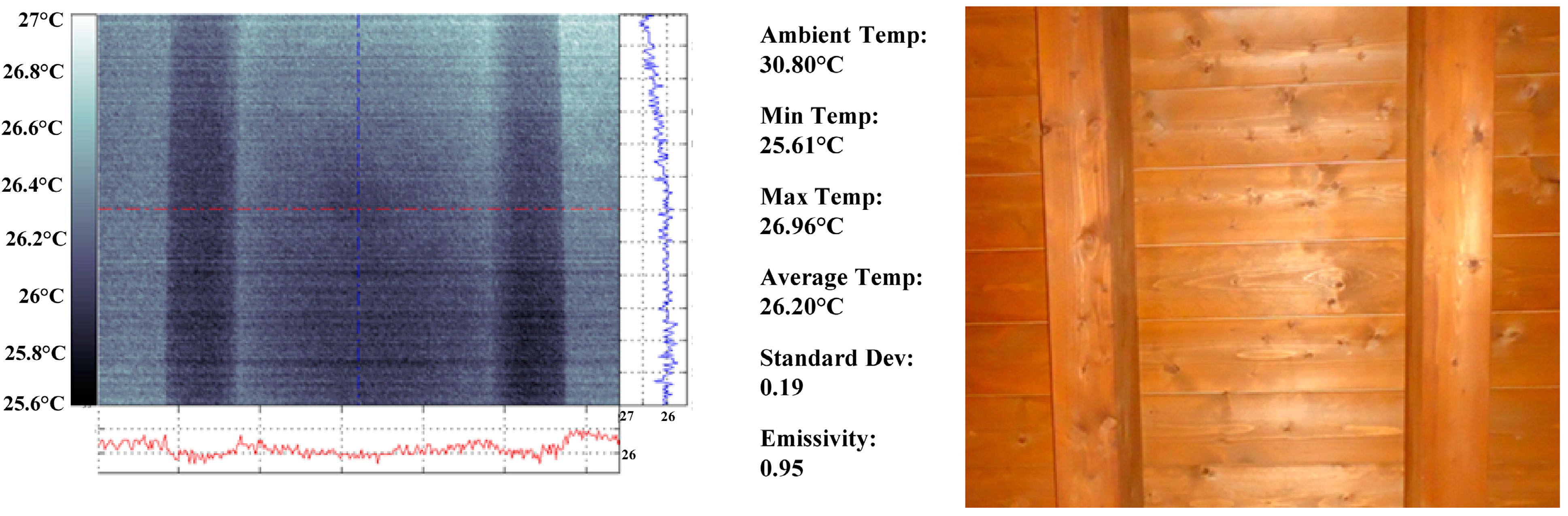
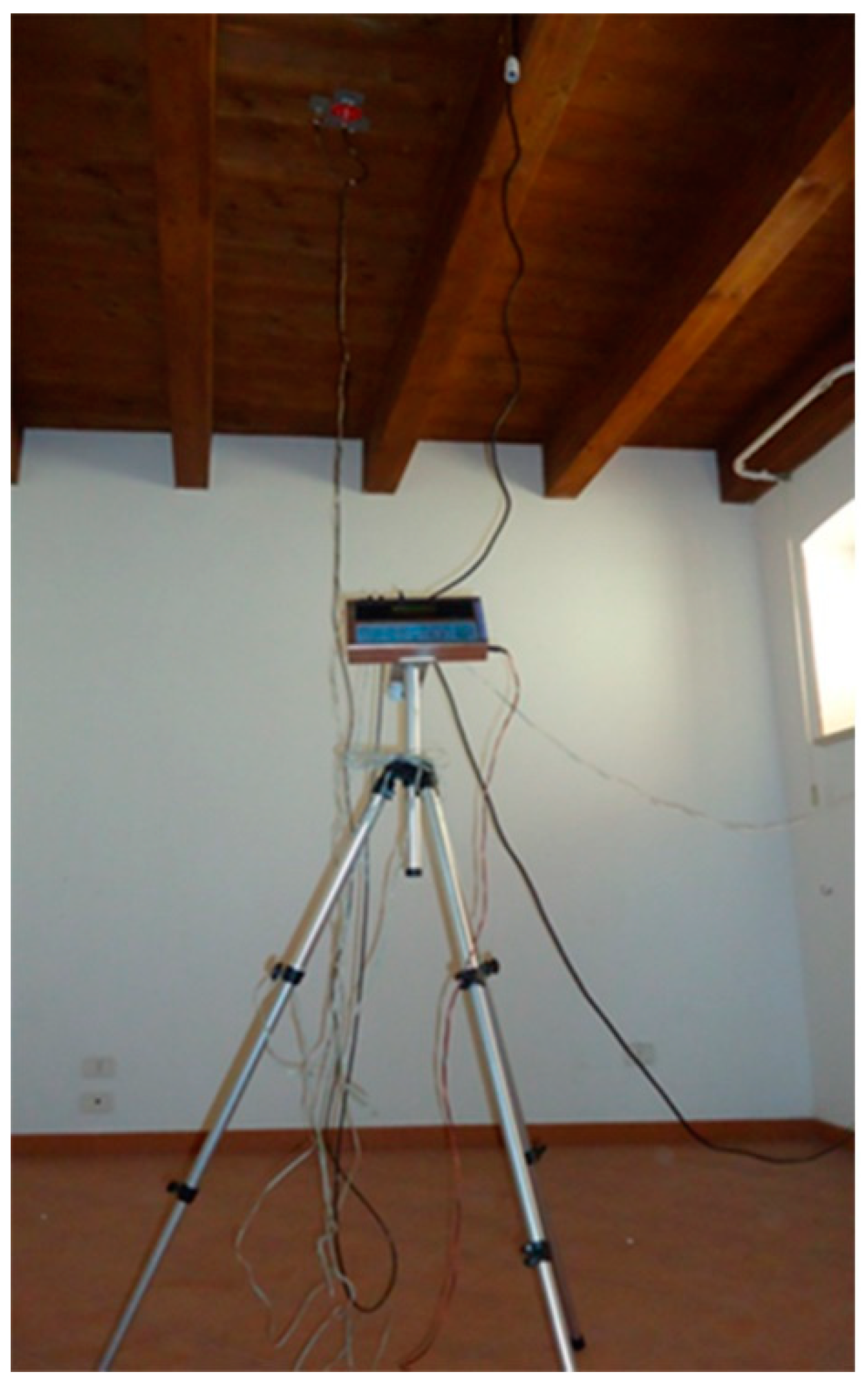
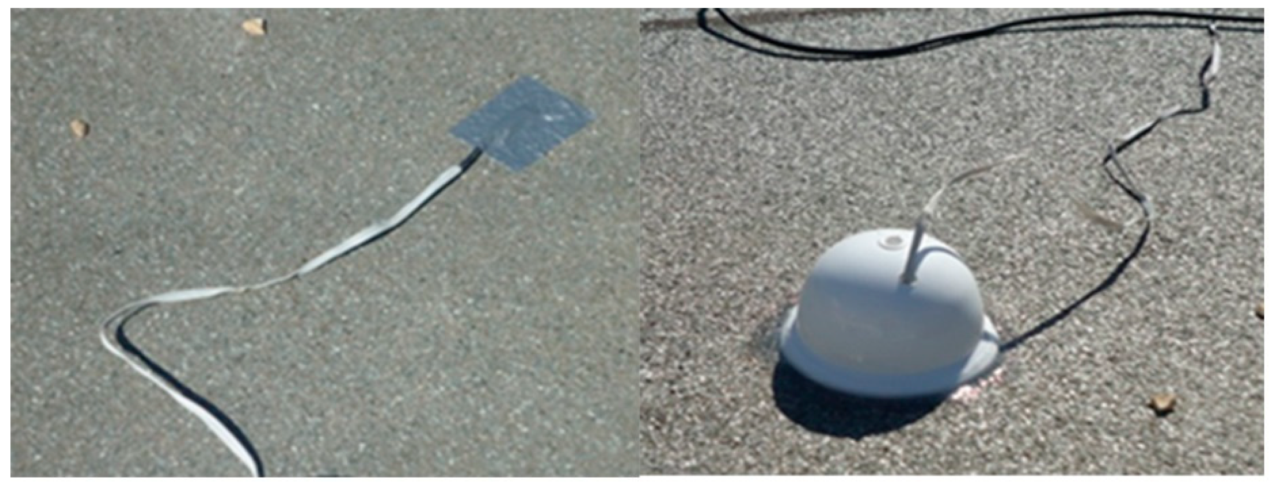
2.2. Onsite Thermal Transmittance Measurements

In order to achieve a reliable model of the building components, the thermal transmittance (U-values) for the roof timber structure and the façade masonry wall of the reference unit were determined experimentally in autumn 2012, following the heat flow meter method as described in ISO 9869-1:1994, then updated by ISO 9869:1-2014 [38].

In detail, the procedure, based on direct measurement of the heat flow rate and temperatures on both sides of the element under steady-state conditions, is mainly effective for plane building components with opaque layers that are perpendicular to the heat flow and have no significant lateral heat flow. Consequently, the selections of the investigation areas should avoid the proximity of thermal anomalies, such as heterogeneous materials, constructional joints, decay of the finishing layers, cracks, and humidity patterns. For this purpose, a preliminary thermographic inspection, which helped localise representative and undisturbed surfaces (Figure 5), was carried out according to EN 13187:1998 [39] by thermo-camera Avio TVS-700P (measurement ranges: −20/500 °C; wavelength: 8/14 μm; thermal resolution: 0.08 °C, thermal accuracy: ±2 °C). Nevertheless, locations close to electric devices, lighting, and space heating and cooling systems, as well as those close to openings, wall corners, and floor/wall and ceiling/wall connections, were avoided (Figure 6).

Once the investigation areas were selected, for both the components, the onsite set-up was installed using LSI-Lastem equipment as follows (Figure 7):

• Heat flow meter BSR240 (range ±50 W/m², resolution 0.1 W/m²) and BST110 flat probes in silver-plated copper (range −50/+80 °C, accuracy ± 0.23 °C at 40 °C) for contact temperature measurements on the internal and external surfaces.
• BST 110 probes (range −50/+80 °C, accuracy ± 0.23 °C at 40 °C) for ambient temperature sensors, indoor and outdoor, respectively.
• Central multi-acquisition reading unit BABUC/A (11 input multiple data device with 20,000 samples memory).

To reduce the thermal break between the support and the plates, the apparatuses were inserted, applying a thermal conducting paste to the back of the plates. Moreover, the external probes were protected against atmospheric agents and direct solar exposure (Figure 8). Finally, to guarantee that the heat flow was unidirectional, it was decided to set the heating system to an average temperature of 30 °C for the masonry and 35 °C for the roof, considering the constant shadows on the external surfaces due to the closeness of the surrounding buildings in the historical centre.

In both cases, data were recorded continuously at fixed intervals of 15 min. Although ISO 9869-1 suggests that measurements should be conducted for at least three days to estimate the U-value of the element, the time interval was extended, as suggested by several authors before and after the investigation year [40,41,42,43]. In detail, the measurements were run from 5 October until 15 October 2012 for the roof and from 6 November until 13 November 2012.

The elaboration method was the average one [44], which assumes that the thermal resistance R is given by dividing the mean surface temperature difference (T_si—T_se) by the thermal flux (q), as follows:

$$R_{AM}=\frac{{{\displaystyle \sum }}_{j=1}^n\left(T_{si,j}-T_{se,j}\right)}{{{\displaystyle \sum }}_{j=1}^n{q}_j}$$

(1)

where R_AM represents the R-value evaluated by the average method (m² K/W), q is the density of the heat flow rate (W/m²), T_si and T_se are the interior and exterior surface temperatures (K), respectively, and index j enumerates the individual measurements.

After a certain time, the R_AM value tends to an asymptote that represents its actual value. Particularly, according to ISO 9869-1, the measurements are reliable when two convergence conditions are fulfilled, beyond the test duration longer than 72 h:

i.

The R-valued obtained at the end of the test (R_AM) does not deviate by more than ±5% from the value obtained 24 h prior to the end of the test (R_AM-24);

ii.

The R-valued obtained by applying the method to the first 67% of the data (R_AM-67%,first) should not deviate by more than ± 5% from the respective value when analysing the last 67% of the data (R_AM-67%,last).

In this specific case, the two conditions were successfully verified (

Table 1. Convergence conditions.

Component	RAM	RAM-24	RAM/RAM-24 Deviation	RAM-67%,first	RAM-67%,last	RAM-67%,first/RAM-67%,last Deviation
Wall	0.960	0.966	−0.6%	0.981	1.028	−4.5%
Roof	1.888	1.901	−0.7%	1.901	1.972	−3.6%

), based on intermediate data downloads.

Thus, the final thermal transmittance was calculated, as follows:

$$U_{AM}=\frac{{{\displaystyle \sum }}_{j=1}^n{q}_j}{{{\displaystyle \sum }}_{j=1}^n\left(T_{i,j}-T_{e,j}\right)}$$

(2)

where U_AM represents the U-value evaluated by the average method (W m⁻² K⁻¹), while T_i and T_e are the interior and exterior air temperature (K), respectively. Moreover, based on the experimental value of the conductance (C_AM), the experimental values of the interior and exterior (R_si,exp and R_se,exp) surface resistances were calculated and compared with the theoretical ones (R_si + R_se), given by ISO 6946:2007 [45] (

Table 2. Experimental values of transmittance, conductance, and surface resistances.

Component	UAM [W m−2 K−1]	CAM (1/RAM) [W m−2 K−1]	Rsi,exp + Rse,exp (1/UAM—1/CAM) [m2 K W−1]	Rsi + Rse [m2 K W−1]
Wall	0.88	1.04	0.17	0.17
Roof	0.42	0.53	0.5	0.14

). It should be observed that the roof shows an experimental value of the overall surface resistance that is higher than the theoretical one. This is reasonably due to local conditions affecting the convective and radiative heat transfer between the component surfaces and the surroundings. Particularly, it might occur because the external air velocity and/or the emissivity of the internal surface are lower than the standard ones (air velocity equal to 4 m/s and internal surface emissivity equal to 0.9, respectively).

Finally, the U-value of the investigated wall, 80 cm thick, was used to determine the U-values for all the different walls of the unit, based on the direct dependency between conductance and thickness (

Table 3. U-values of all the walls of the building.

Thickness (m)	U (W m−2 K−1)
0.90	0.80
0.80	0.88
0.70	0.98
0.60	1.12
0.55	1.20
0.30	2.06

).

3. Materials and Methods

As introduced in Section 2.1, the selected building is highly representative of the historical centre of Molfetta and, more in general, of the coastal historical centres in South Italy. Thus, the procedures and results described have great potential of replicability.

In fact, the old town of Molfetta is a compact aggregate on a peninsula, surrounded by the sea and facing the modern city only on the south side (Figure 9). As documented in previous studies [5], it is characterised by about 63% of three-floor buildings. One of the main building typologies is the palace-house—about 27%—while the predominant construction solutions are stone masonry walls—more than 70%—and roof reinforced concrete/wooden slab—about 65%.

The retrofitting interventions in the historical centre are regulated by a specific plan, released in 1994 and including recommendations for an onsite investigation of the actual performances in order to address suitable and compatible measures. Nevertheless, this part of the city is included in the “Sustainable Energy Action Plan” (SEAP), a strategic document to guide and support local implementation of sustainable energy policies under the European “Covenant of Mayors” Framework. Consequently, methods and tools to guarantee appropriate performance assessment are highly desirable to identify future actions.

Following the methodological framework included in Figure 1 and in line with other studies found in the literature [46,47], after having performed the monitoring campaign to determine the thermal characteristics of the building envelope, the selected building was modelled in DesignBuilder version 6.0.1, and dynamic energy simulations were performed in EnergyPlus version 9.2. In order to optimize the accuracy and the computational resources required by EnergyPlus, a heat balance algorithm using the Conduction Transfer Function (CTF) was used. Moreover, to account for the indoor and outdoor surface convection, the TARP algorithm and the DOE-2 model were used, respectively. Finally, a full exterior solar distribution was considered. The main setup parameters for the simulation of the building in EnergyPlus are included in the following

Table 4. Key case simulation setup.

Parameters	Value
Simulation control
Zone sizing calculation	Yes
System sizing calculation	Yes
Run simulations for weather file run periods	Yes
Building
Solar distribution	Full exterior
Maximum number of warmup days	25
Minimum number of warmup days	6
Shadow calculation
Shadow calculation	Average over days in frequency
Calculation frequency	20
Sky diffuse model algorithm	Simple sky diffuse modeling
Surface convection algorithm: Inside
Surface convection algorithm: Inside	TARP
Surface convection algorithm: Outside
Surface convection algorithm: Outside	DOE-2
Heat balance algorithm
Heat balance algorithm	Conduction Transfer Function (CTF)
Timestep
Number of timesteps per hour	6
Convergence limits
Minimum system timestep (minutes)	1
Run period
Begin month	1
Begin day	1
End month	12
End day	31

.

Although, to properly account for shadings and radiative exchanges within the neighbourhood, the full building and the neighbouring ones were modelled, and the analyses were concentrated on the two bedrooms (LM1 and LS1) of one of the two top floor apartments. Dynamic energy simulations were performed and, in order to assess changes in thermal comfort conditions as a variation of natural ventilation strategies, heating, ventilation, and air conditioning (HVAC) systems were kept switched off for the entire duration of the simulation.

The simulations considered three different cases of window operation:

(a)

Windows are kept closed, and hourly ventilation is provided to ensure a constant ventilation rate of 0.3 ACH, as required by the standard.

(b)

Windows are operated according to a simple rule-based model:

$$if T_{in}>T_{out} windows are opened$$

(3)

This model is intended to provide the maximum potential cooling through ventilation, as at every time-step where outdoor fresh air is available, natural ventilation is provided. We decided to consider a rule-based model based only on indoor and outdoor temperatures to simplify the interpretation of results. Moreover, according to several studies [48,49], indoor and outdoor temperatures are the main drivers for occupant window opening behaviours and are used in similar studies [50,51].

(c)

Implementation of a stochastic model.

The stochastic model was employed to evaluate user behaviour inside the building. The model developed by Jones et al. [23], based on Markov chain based logistic regression, was adopted in order to account for users’ operational behaviour of windows. The stochastic model was developed with measurements made in ten buildings in UK for a period of one year. The study used a multivariate logistic regression to obtain the probability of opening and closing the windows, evaluating it through internal and external environmental factors, according to the time of day and the season. The model indicates how the opening and closing operations are linked to a range of environmental variables (indoor and outdoor air temperature, indoor and outdoor relative humidity, wind speed, solar radiation, and precipitation) and contextual (season, hour of the day). Furthermore, it was observed that the effects of environmental variables varied based on contextual factors. The model calculated the probability of opening or closing the window in the next ten minutes. The analysis, as mentioned above, was conducted using a logistic regression. The relationship between the probability of the binary result and the individual explanatory variables can be expressed by the univariate linear logistic regression, represented by the following equation:

$$P\left(x\right)=\frac{1}{1+e^{-\left(\alpha +\beta x\right)}}, P\left(x\right)\epsilon \left[0,1\right]\forall x$$

(4)

where P(x), or simply p, is the probability of the binary result, α is the intercept, β is a coefficient, and x is the explanatory variable such as, for example, air temperature, wind speed, etc.

The regression was used to establish the probability of opening or closing the main bedroom window, considering various internal and external environmental variables.

The following Equation (4) represents the relationship between p and several selected environmental variables:

$$ln\left(\frac{p}{1-p}\right)=\alpha +{\beta }_0{x}_0+{\beta }_1{x}_1+\dots +{\beta }_n{x}_n$$

(5)

In the model of Jones, the following variables were considered as significant for the probability of the operation of windows: (i) indoor temperature (t_in), (ii) indoor relative humidity (RH_in), (iii) outdoor temperature (t_out), (iv) outdoor relative humidity (RH_out), (v) wind speed (WS), and (vi) rainfall (RF). Therefore, the model consists of two logistic regressions, which were used to calculate the probabilities of opening and closing windows. The probability of opening was calculated first, then the probability of closing, and finally the initial state of the window was evaluated.

$$ln{\left(\frac{p}{1-p}\right)}_{opening}=-9.275+0.233t_{in}+0.038R{H}_{in}-0.105t_{out}-0.042R{H}_{out}+0.057WS+0.034RF$$

(6)

$$ln{\left(\frac{p}{1-p}\right)}_{closing}=-2.984-0.178t_{in}-0.017R{H}_{in}+0.062t_{out}+0.063WS+0.032RF$$

(7)

Then, an EnergyPlus Energy Management System (EMS) routine was compiled to simulate the stochastic behaviour of occupants. If the initial state of the window was closed, the occupation of the bedrooms analysed was greater than 1, and the probability of opening was greater than the probability of closing, then the program would define the window as open, and on the contrary it remains closed. If the initial state of the window was closed, the occupancy of the bedrooms was equal to zero, and the probability of closure was greater than the one of opening, then the program would define the window as closed.

The results of simulations were, then, used to assess indoor thermal comfort conditions. The thermal comfort assessment was carried out through the European standard EN 16798-1 [52]. Indoor conditions able to meet Class I comfort requirements were considered. Comfort assessment was performed in the summer period (1 June–30 September), and the analyses were concentrated on the two bedrooms of the second floor (ref. Figure 1, double occupancy bedroom LM1 and single occupancy bedroom LS1).

For the assessment of the thermal conditions in buildings, several long-term thermal discomfort indices are available in the literature [53]. In this study, the daily discomfort degree hours (DDH) and daily percentage of discomfortable hours (%DH) were adopted. DDH and %DH were calculated according to the following Equations (8) and (9):

$$DDH={{\displaystyle \sum }}_{i=1}^{24}\left(T_{O,in}-T_C\right) \forall T_{O,in}>T_C$$

(8)

$$\%DH=\frac{{{\displaystyle \sum }}_{i=1}^{24}\left(T_{O,in}-T_C\right)}{24} \forall T_{O,in}>T_C$$

(9)

where T_O,in is the hourly value of indoor operative temperature, and T_C is the daily upper limit of the thermal comfort band, calculated according to EN 16798-1 for the thermal comfort class I. The thermal comfort assessment was based only on indoor operative temperatures, since relative humidity and air speed in indoor spaces do not vary significantly as a variation of weather conditions and of models adopted.

In order to account for changes between current and future scenarios [54], three weather conditions were simulated, and the thermal comfort levels of the two selected rooms were consequently calculated:

(1)

Typical Meteorological Year. The method for creating TMY files was developed by Hall et al. [55] in 1978. The most representative month is selected for each of the twelve months of the year for several years of observation. The twelve months are then combined in a typical year called TMY. The advantage of this method lies in the fact that the calculations are reduced, given that one year describes the trend of 20–30 years, while in any case the most representative conditions are taken into consideration. The biggest disadvantage concerns the fact that extreme events are underestimated, as the process generates an average of the events [56]. For the simulations of thermal comfort in TMY conditions, the database developed by Politecnico di Milano, namely known as Italian Climatic Data Collection “Gianni De Giorgi” (IGDG), was used. Therefore, in the following paragraphs, this condition is identified as “IGDG”. The IGDG dataset was generated from data recorded in the period 1951–1970, therefore not accounting for the climate changes that occurred in the last 50 years [1]. We decided to use TMY as a basis for future projections, as it is widely known as the most reliable [57] and is largely used in other similar studies, thus ensuring the comparability of results of our study with other ones.

(2)

Current extreme meteorological conditions. According to the Italian National Research Council (CNR), 2018 was the hottest year for Italy since 1800 [58] and up to the period when this study was performed. For this reason, a meteorological file of 2018 was created using the EnergyPlus Weather (EPW) format. Basic climatic data were obtained from the Regional Environmental Protection Agency (ARPA) for the closest city (Bari, 30 km far from Molfetta) [59]. As only global solar radiation values are available from ARPA, its direct and diffuse components were generated through the method developed by Watanabe et al. [60]. In the following paragraphs, the current extreme meteorological condition is referred to as “Extreme (2018)”.

(3)

Future meteorological conditions. The statistical downscaling method was used to derive future meteorological conditions. A tool developed by Jentsch et al. was used [61]. The tool allows for the generation of future climate files for different places in the world. The chosen output on which the tool’s operating methodology is based is HadCM3, is forced with the A2 scenario, and is developed by the IPCC [62]. Future meteorological conditions were generated for three periods: 2011–2040 (referred to in the following paragraphs as “Average (2020)”), 2041–2070 (referred to as “Average (2050)”), and 2071–2100 (referred to as “Average (2080)”).

4. Results and Discussion

Figure 10 summarises the progress of the seasonal total number of discomfort hours in future weather scenarios. For each of the two rooms analysed, the two models (rule-based—plotted in blue—and stochastic—plotted in red) were compared. In the figure, together with the results of single-year analyses, a regression line is presented, in order to forecast for variations in discomfort conditions in time scenarios outside the current assessment.

From the analysis of the results, it can be highlighted that DDH, based on the TMY (1951–1970), were between 25.6 °C and 306.2 °C, depending on the room and on the model, with a percentage of days with discomfortable conditions between 32–41% for the double-occupancy room and between 6–9% for the single occupancy room. Differences between the two rooms are due to the higher internal gains and solar gains for the double occupancy room in comparison to the single occupancy room. Moreover, the analyses based on TMY showed a significant difference in the amplitude of discomfort if calculated by means of rule-based or stochastic models, with the latter predicting about half of DDH as compared to the rule-based model (25.6 °C against 55.3 °C for the single occupancy room and 119.2 °C against 306.2 °C for the double occupancy room), but there were no significant differences in days with unacceptable comfort conditions. This is because the adoption of a more detailed strategy of control of natural ventilation (achieved by using stochastic models) tends to maximise the benefits of thermal mass and cross ventilation with evident advantages in traditional masonry buildings.

From the analysis of trend lines included in Figure 10, it is evident how the trend of discomfort degree hours follows an exponential pattern for all conditions, with a substantial increase of discomfort for too hot conditions by 2080, compared to the conditions assessed by means of the TMY. However, while the pattern of variations by the adoption of the two models is similar, it is equally evident how the rule-based model (blue line) tends to overestimate discomfort conditions in comparison with stochastic one (red lines). Focusing on the “2080” scenario, the DDH in the two rooms were between 70–74% higher when a rule-based model of window operation was used in comparison to a stochastic one. Furthermore, more limited—although still significant—variations of percentage of days with discomfortable hours (variable between 4–10%) can be found with the adoption of the two models.

By focusing on the ability of the two models to predict thermal discomfort, the analysis showed that the adoption of a rule-based model tends to overestimate thermal discomfort conditions, since it is based on fixed scheduled rules, such as the ventilation rate provided by the legislation. On the contrary, the stochastic model led to lower values of DDH, as it considered the users’ behaviour, which can adapt the indoor environment to their needs. In detail, the stochastic model considered the window operational behaviour, allowing a more accurate strategy of control of natural ventilation. Therefore, unlike the rule-based model, the benefits related to the cross ventilation can be maximised, resulting in lower values of operative temperatures, and thus of DDH. The discrepancy between rule-based and stochastic models can be pointed out in both the current and the future weather scenarios. The implications of this analysis are bifold. On one hand, the analysis gives an insight to designers and researchers on how to model windows’ operations in naturally ventilated historic buildings and on how stochastic models can predict more realistic comfort conditions. Secondly, the results highlight that, in future weather scenarios, stochastic models—in comparison to deterministic ones—are able to predict more accurately the changes in behaviours of occupants and their ability to adapt to changed outdoor environmental conditions.

The DDH calculated based on the extreme weather file recorded in 2018 are depicted in Figure 11, along with the DDH trend lines based on the predicted future weather files, previously shown in Figure 10. Once again, the two models (rule-based—plotted in light and dark blue—and stochastic—plotted in light and dark red) were compared for both the bedrooms. Overall, some discrepancies can be pointed out between DDH based on real data and those based on predicted data in both the zones. In detail, in the double-occupancy bedroom, predicted weather files tended to underestimate DDH values, whereas in the single-occupancy bedroom, predicted climate files resulted in an overestimation of DDH values, compared with the recorded file. Furthermore, the magnitude of these differences varied depending on the occupant behaviour model adopted: stochastic models showed smaller differences compared to rule-based ones. Indeed, the stochastic model presented limited differences between HDDs calculated with real-time weather data and predicted ones, compared to rule-based ones, being capable of characterizing the dynamic behaviour of the building.

Further considerations can be drawn focusing on the percentage of daily number of discomfort hours experienced by each bedroom, reported in Figure 12. In this figure, the results of all the analyses conducted are overlapped to identify the different trends. Hence, the darkest red areas describe periods of the year where all the models (IGDG, 2020, 2050, 2080) were affected by thermal discomfort, while brighter areas refer only to certain scenarios (respectively 2020–2050–2080, 2050–2080, 2080). Both the double-occupancy bedroom (Figure 12a) and the single-occupancy bedroom (Figure 12b) show the same increasing trend in daily %DH as time goes by. This upward trend is characterised by the rise of number of days characterised by thermal discomfort, as well as by the rise of the discomfort hours in a day. Nevertheless, the single-occupancy bedroom appeared to experience lower values of %DH, spread over a smaller number of days.

More in detail, referring to the double occupancy bedroom, the majority of days (68%) did not show any %DH in the past, computed according to TMY. Indeed, only 40 days out of 122 experienced discomfort, spread over the last week of June, the last week of July, and the second week of August. The %DH ranged between 10–60%, with the most frequent value of 40% and a peak value of 58% on the 25 July. In 2020, most days were still not affected by discomfort hours (57%), although this percentage decreased by roughly 10%. Therefore, the number of days experiencing discomfort increased, and are approximately distributed from the last week of June until mid-August. The values of daily %DH increased, with the most frequent values of 40–50% and peak values of up to 80%. The same trend can be observed in 2050, with a progressive growth in the number of days with discomfort, as well as in the percentage of daily %DH (in this case up to 90%). Unlike the three previous scenarios, in 2080, the number of days that do not experience discomfort narrow down to 11%; therefore, the majority of days show daily %DH, distributed from mid-June until the last week of September. The daily %DH rises, with the most frequent value being 80% (21% of days) and as many as 11% reaching 100% of %DH.

Similar patterns can be recognised referring to the single-occupancy bedroom.

Overall, due to the rising temperatures, the %DH appeared to increase as the time goes by, both in the %DH experienced in a day and in the number of days characterised by discomfort conditions. Starting from sporadic, fragmented, and low-magnitude discomfort phenomena, the %DH reaches higher values and increases its frequencies as temperatures rise. Therefore, although it provides a more accurate assessment of the buildings’ behaviour, the stochastic model did not ensure adequate comfort levels due to rising temperatures. However, it can be considered as a starting point to develop other passive strategies.

5. Conclusions

In this work, the indoor thermal conditions in a historical residential building in the summer period were assessed by means of stochastic and rule-based window operation models. In addition, the future patterns of indoor thermal comfort due to climate change were evaluated using the stochastic model.

The overarching aim of the study was to compare how behavioural changes evaluated by means of rule-based and stochastic models lead to changes in the regime of indoor operative temperatures and how to define the patterns of indoor thermal comfort in historic residential buildings in future years, by using a stochastic model.

To this scope, a historic residential building located in Molfetta (Southern Italy—Mediterranean climate) was modelled and simulated in a dynamic energy simulation software. The simulations were limited to the summer period (1 June–31 September), in five weather conditions: (i) the current climate (IGDG weather file), (ii) an extreme weather file based on the climate variables recorded in 2018, (iii) short-term scenario (2020), (iv) mid-term scenario (2050), and (v) long-term scenario (2080). The simulations were carried out separately for two thermal zones: a single-occupancy bedroom and a double-occupancy bedroom.

Unlike the rule-based comfort model, which is based on fixed rules (ventilation rate provided by legislation), the stochastic model provided a more reliable description of the reality, including the aleatory uncertainties related to user operation of the windows. The analyses showed that the adoption of a stochastic model enabled the characterization of the dynamic interaction of the occupants with the building in all the weather scenarios, since it considered the users’ behaviour, expressed by the probability of opening or closing windows, as expected, considering that the window opening control leads to a reduction of discomfort levels in all climatic conditions. Nevertheless, although these comfort conditions improved compared to those based on the rule-based model, they were still not acceptable in the medium and long-term weather scenarios, due to the significant increase in temperatures caused by climate change. Therefore, the stochastic model can be used as a baseline to develop detailed strategies for climate change adaptation. Considering the results obtained and that existing buildings are required to be refurbished to meet the European recommendations, the stochastic model appears to be a reliable tool to address, at least partially, the issue of the performance gap between the simulated and actual energy behaviours of buildings.

This work is intended to be a starting point for further works aimed at investigating the thermal behaviour of new buildings compared to existing ones, as well as the differences between different climate zones. Although the building typology selected was demonstrated to be representative of recurrent typologies of existing masonry buildings built in the Mediterranean area, the results were limited to the specific typology and climate assessed and did not include any predictions on the effects of interventions of refurbishment or of energy retrofit. Therefore, the research was not intended to be conclusive, nor was it intended to be unique, but it can be considered a useful basis to search for new solutions to improve the energy performance of buildings.

References

1. IPCC. Global Warming of 1.5 °C. An IPCC Special Report on the Impacts of Global Warming of 1.5 °C above Pre-Industrial Levels and Related Global Greenhouse Gas Emission Pathways, in the Context of Strengthening the Global Response to the Threat of Climate Change, Sustainable Development, and Efforts to Eradicate Poverty; IPCC: Geneva, Switzerland, 2018. [Google Scholar]
2. Pagliano, L.; Carlucci, S.; Causone, F.; Moazami, A.; Cattarin, G. Energy retrofit for a climate resilient child care centre. Energy Build. 2016, 127, 1117–1132. [Google Scholar] [CrossRef]
3. Thiébault, S.; Moatti, J.-P.; Ducrocq, V.; Gaume, E.; Dulac, F.; Hamonou, E.; Shin, Y.-J.; Joel, G.; Boulet, G.; Guégan, J.; et al. The Mediterranean Region under Climate Change. A Scientific Update; IRD Editions: Montpellier, France, 2016. [Google Scholar]
4. European Commission. Climate Actions. Available online: https://ec.europa.eu/clima/citizens/eu_en (accessed on 4 May 2020).
5. De Fino, M.; Scioti, A.; Cantatore, E.; Fatiguso, F. Methodological framework for assessment of energy behavior of historic towns in Mediterranean climate. Energy Build. 2017, 144, 87–103. [Google Scholar] [CrossRef]
6. Webb, A.L. Energy retrofits in historic and traditional buildings: A review of problems and methods. Renew. Sustain. Energy Rev. 2017, 77, 748–759. [Google Scholar] [CrossRef]
7. Caro, R.; Sendra, J.J. Are the dwellings of historic Mediterranean cities cold in winter? A field assessment on their indoor environment and energy performance. Energy Build. 2021, 230, 110567. [Google Scholar] [CrossRef]
8. Berg, F.; Flyen, A.-C.; Godbolt, Å.L.; Broström, T. User-driven energy efficiency in historic buildings: A review. J. Cult. Herit. 2017, 28, 188–195. [Google Scholar] [CrossRef] [Green Version]
9. van Vuuren, D.P.; Edmonds, J.; Kainuma, M.; Riahi, K.; Thomson, A.; Hibbard, K.; Hurtt, G.C.; Kram, T.; Krey, V.; Lamarque, J.F.; et al. The representative concentration pathways: An overview. Clim. Chang. 2011, 109, 5–31. [Google Scholar] [CrossRef]
10. Moazami, A.; Nik, V.M.; Carlucci, S.; Geving, S. Impacts of future weather data typology on building energy performance–Investigating long-term patterns of climate change and extreme weather conditions. Appl. Energy 2019, 238, 696–720. [Google Scholar] [CrossRef]
11. Belcher, S.E.; Hacker, J.N.; Powell, D.S. Constructing design weather data for future climates. Build. Serv. Eng. Res. Technol. 2005, 26, 49–61. [Google Scholar] [CrossRef]
12. IEA-EBC Annex 66. Definition and Simulation of Occupant Behavior in Buildings. Available online: https://annex66.org/ (accessed on 4 May 2020).
13. Carlucci, S.; De Simone, M.; Firth, S.K.; Kjærgaard, M.B.; Markovic, R.; Rahaman, M.S.; Annaqeeb, M.K.; Biandrate, S.; Das, A.; Dziedzic, J.W.; et al. Modeling occupant behavior in buildings. Build. Environ. 2020, 174, 106768. [Google Scholar] [CrossRef]
14. Vellei, M.; Azar, E.; Bandurski, K.; Berger, C.; Carlucci, S.; Dong, B.; Favero, M.; Mahdavi, A.; Schweiker, M. Documenting occupant models for building performance simulation: A state-of-the-art. J. Build. Perform. Simul. 2022, 15, 634–655. [Google Scholar] [CrossRef]
15. Hoes, P.; Hensen, J.L.M.; Loomans, M.G.L.C.; de Vries, B.; Bourgeois, D. User behavior in whole building simulation. Energy Build. 2009, 41, 295–302. [Google Scholar] [CrossRef] [Green Version]
16. Schweiker, M.; Haldi, F.; Shukuya, M.; Robinson, D. Verification of stochastic models of window opening behaviour for residential buildings. J. Build. Perform. Simul. 2012, 5, 55–74. [Google Scholar] [CrossRef]
17. Haldi, F.; Robinson, D. On the behaviour and adaptation of office occupants. Build. Environ. 2008, 43, 2163–2177. [Google Scholar] [CrossRef]
18. Herkel, S.; Knapp, U.; Pfafferott, J. Towards a model of user behaviour regarding the manual control of windows in office buildings. Build. Environ. 2008, 43, 588–600. [Google Scholar] [CrossRef]
19. Haldi, F.; Robinson, D. Interactions with window openings by office occupants. Build. Environ. 2009, 44, 2378–2395. [Google Scholar] [CrossRef]
20. Rijal, H.B.; Tuohy, P.; Nicol, F.; Humphreys, M.A.; Samuel, A.; Clarke, J. Development of an adaptive window-opening algorithm to predict the thermal comfort, energy use and overheating in buildings. J. Build. Perform. Simul. 2008, 1, 17–30. [Google Scholar] [CrossRef] [Green Version]
21. Rijal, H.B.; Tuohy, P.; Humphreys, M.A.; Nicol, J.F.; Samuel, A.; Clarke, J. Using results from field surveys to predict the effect of open windows on thermal comfort and energy use in buildings. Energy Build. 2007, 39, 823–836. [Google Scholar] [CrossRef] [Green Version]
22. Yun, G.Y.; Steemers, K. Time-dependent occupant behaviour models of window control in summer. Build. Environ. 2008, 43, 1471–1482. [Google Scholar] [CrossRef]
23. Jones, R.V.; Fuertes, A.; Gregori, E.; Giretti, A. Stochastic behavioural models of occupants’ main bedroom window operation for UK residential buildings. Build. Environ. 2017, 118, 144–158. [Google Scholar] [CrossRef]
24. Reinhart, C.F. Lightswitch-2002: A model for manual and automated control of electric lighting and blinds. Sol. Energy 2004, 77, 15–28. [Google Scholar] [CrossRef] [Green Version]
25. Nicol, J.F. Characterising occupant behavior in buildings: Towards a stochastic model of occupant use of windows, lights, blinds, heaters and fans. In Proceedings of the Seventh International IBPSA Conference, Rio de Janeiro, Brazil, 13–15 August 2001; pp. 1073–1078. [Google Scholar]
26. Martínez-Molina, A.; Tort-Ausina, I.; Cho, S.; Vivancos, J.L. Energy efficiency and thermal comfort in historic buildings: A review. Renew. Sustain. Energy Rev. 2016, 61, 70–85. [Google Scholar] [CrossRef]
27. Cardinale, N.; Rospi, G.; Stefanizzi, P. Energy and microclimatic performance of Mediterranean vernacular buildings: The Sassi district of Matera and the Trulli district of Alberobello. Build. Environ. 2013, 59, 590–598. [Google Scholar] [CrossRef]
28. De Berardinis, P.; Rotilio, M.; Marchionni, C.; Friedman, A. Improving the energy-efficiency of historic masonry buildings. A case study: A minor centre in the Abruzzo region, Italy. Energy Build. 2014, 80, 415–423. [Google Scholar] [CrossRef]
29. Balocco, C.; Grazzini, G. Numerical simulation of ancient natural ventilation systems of historical buildings. A case study in Palermo. J. Cult. Herit. 2009, 10, 313–318. [Google Scholar] [CrossRef]
30. Cantin, R.; Burgholzer, J.; Guarracino, G.; Moujalled, B.; Tamelikecht, S.; Royet, B.G. Field assessment of thermal behaviour of historical dwellings in France. Build. Environ. 2010, 45, 473–484. [Google Scholar] [CrossRef]
31. Hao, L.; Herrera-Avellanosa, D.; Del Pero, C.; Troi, A. What Are the Implications of Climate Change for Retrofitted Historic Buildings? A Literature Review. Sustainability 2020, 12, 7557. [Google Scholar]
32. Lee, W.V.; Steemers, K. Exposure duration in overheating assessments: A retrofit modelling study. Build. Res. Inf. 2017, 45, 60–82. [Google Scholar] [CrossRef] [Green Version]
33. Peacock, A.D.; Jenkins, D.P.; Kane, D. Investigating the potential of overheating in UK dwellings as a consequence of extant climate change. Energy Policy 2010, 38, 3277–3288. [Google Scholar] [CrossRef]
34. Escandón, R.; Suárez, R.; Sendra, J.J.; Ascione, F.; Bianco, N.; Mauro, G.M. Predicting the Impact of Climate Change on Thermal Comfort in A Building Category: The Case of Linear-type Social Housing Stock in Southern Spain. Energies 2019, 12, 2388. [Google Scholar] [CrossRef] [Green Version]
35. Ben, H.; Steemers, K. Energy retrofit and occupant behaviour in protected housing: A case study of the Brunswick Centre in London. Energy Build. 2014, 80, 120–130. [Google Scholar] [CrossRef]
36. UNI/TR 11552; Abaco delle Strutture Costituenti l’involucro Opaco Degli Edifici-Parametri Termofisici. UNI: Milan, Italy, 2014. Available online: https://www.uni.com/index.php?option=com_content&view=article&id=2419:abaco-delle-strutture-costituenti-l-involucro-opaco-degli-edifici&Itemid=2279 (accessed on 12 May 2020).
37. Fatiguso, F.; De Fino, M.; Cantatore, E. An energy retrofitting methodology of Mediterranean historical buildings. Manag. Environ. Qual. Int. J. 2015, 26, 984–997. [Google Scholar] [CrossRef]
38. ISO 9869-1; Thermal Insulation. Building Elements. In-Situ Measurement of Thermal Resistance and Thermal Transmittance Heat Flow Meter Method. ISO: Genève, Switzerland, 2014.
39. EN 13187; Thermal Performance of Buildings-Qualitative Detection of Thermal Irregularities in Building Envelopes-Infrared Method. CEN: Brussels, Belgium, 1998.
40. Desogus, G.; Mura, S.; Ricciu, R. Comparing different approaches to in situ measurement of building components thermal resistance. Energy Build. 2011, 43, 2613–2620. [Google Scholar] [CrossRef]
41. Lucchi, E. Thermal transmittance of historical stone masonries: A comparison among standard, calculated and measured data. Energy Build. 2017, 151, 393–405. [Google Scholar] [CrossRef]
42. Atsonios, I.A.; Mandilaras, I.D.; Kontogeorgos, D.A.; Founti, M.A. A comparative assessment of the standardized methods for the in–situ measurement of the thermal resistance of building walls. Energy Build. 2017, 154, 198–206. [Google Scholar] [CrossRef]
43. Teni, M.; Krstić, H.; Kosiński, P. Review and comparison of current experimental approaches for in-situ measurements of building walls thermal transmittance. Energy Build. 2019, 203, 109417. [Google Scholar] [CrossRef]
44. Choi, D.S.; Ko, M.J. Analysis of Convergence Characteristics of Average Method Regulated by ISO 9869-1 for Evaluating In Situ Thermal Resistance and Thermal Transmittance of Opaque Exterior Walls. Energies 2019, 12, 1989. [Google Scholar] [CrossRef] [Green Version]
45. ISO 6946; Building Components and Building Elements–Thermal Resistance and Thermal Transmittance–Calculation Method. ISO: Genève, Switzerland, 2007.
46. Ozarisoy, B. Energy effectiveness of passive cooling design strategies to reduce the impact of long-term heatwaves on occupants’ thermal comfort in Europe: Climate change and mitigation. J. Clean. Prod. 2022, 330, 129675. [Google Scholar] [CrossRef]
47. Guerrero Delgado, M.; Sánchez Ramos, J.; Palomo Amores, T.R.; Castro Medina, D.; Álvarez Domínguez, S. Improving habitability in social housing through passive cooling: A case study in Mengíbar (Jaén, Spain). Sustain. Cities Soc. 2022, 78, 103642. [Google Scholar] [CrossRef]
48. Roetzel, A.; Tsangrassoulis, A.; Dietrich, U.; Busching, S. A review of occupant control on natural ventilation. Renew. Sustain. Energy Rev. 2010, 14, 1001–1013. [Google Scholar] [CrossRef]
49. Fabi, V.; Andersen, R.V.; Corgnati, S.; Olesen, B.W. Occupants’ window opening behaviour: A literature review of factors influencing occupant behaviour and models. Build. Environ. 2012, 58, 188–198. [Google Scholar] [CrossRef]
50. Rinaldi, A.; Roccotelli, M.; Mangini, A.M.; Fanti, M.P.; Iannone, F. Natural Ventilation for Passive Cooling by Means of Optimized Control Logics. Procedia Eng. 2017, 180, 841–850. [Google Scholar] [CrossRef]
51. Tang, L.; Ai, Z.; Song, C.; Zhang, G.; Liu, Z. A Strategy to Maximally Utilize Outdoor Air for Indoor Thermal Environment. Energies 2021, 14, 3987. [Google Scholar] [CrossRef]
52. EN 16798-1; Energy performance of buildings-Ventilation for buildings-Part 1: Indoor environmental input parameters for design and assessment of energy performance of buildings addressing indoor air quality, thermal environment, lighting and acoustics. CEN: Brussels, Belgium, 2019.
53. Carlucci, S.; Pagliano, L. A review of indices for the long-term evaluation of the general thermal comfort conditions in buildings. Energy Build. 2012, 53, 194–205. [Google Scholar] [CrossRef]
54. Rodrigues, E.; Fernandes, M.S. Overheating risk in Mediterranean residential buildings: Comparison of current and future climate scenarios. Appl. Energy 2020, 259, 114110. [Google Scholar] [CrossRef]
55. Hall, I.J.; Prairie, R.R.; Anderson, H.E.; Boes, E.C. Generation of a Typical Meteorological Year; Sandia Labs.: Albuquerque, NM, USA, 1978. [Google Scholar]
56. Nik, V.M. Making energy simulation easier for future climate-Synthesizing typical and extreme weather data sets out of regional climate models (RCMs). Appl. Energy 2016, 177, 204–226. [Google Scholar] [CrossRef]
57. Crawley, D.B. Which Weather Data Should You Use for Energy Simulations of Commercial Buildings? ASHRAE Trans. 1998, 104, 498–515. [Google Scholar]
58. CNR-ISAC. Press Note of 7 January 2019. Available online: https://www.cnr.it/it/nota-stampa/n-8503/cnr-isac-2018-anno-piu-caldo-dal-1800-per-l-italia (accessed on 12 May 2020).
59. ARPA Puglia. Official Website. Available online: www.arpa.puglia.it (accessed on 21 April 2020).
60. Watanabe, T.; Urano, Y.; Hayashi, T. Procedures for separating direct and diffuse insolation on a horizontal surface and prediction of insolation on tilted surfaces. Trans. Archit. Inst. Jpn. 1983, 330, 96–108. [Google Scholar] [CrossRef] [Green Version]
61. Jentsch, M.F.; James, P.A.B.; Bourikas, L.; Bahaj, A.S. Transforming existing weather data for worldwide locations to enable energy and building performance simulation under future climates. Renew. Energy 2013, 55, 514–524. [Google Scholar] [CrossRef]
62. IPCC. Climate Change 2014: Syntesis Report. Contribution of Working Groups I, II and III to the Fifth Assessment Report of the Intergovernmental Panel on Climate Change; IPCC: Geneva, Switzerland, 2014; p. 151. [Google Scholar]
Figure 1. Conceptual framework of the study.
Energies 15 04984 g001
Figure 2. Typical floorplan of the selected building.
Energies 15 04984 g002
Figure 3. Main elevation of the selected building.
Energies 15 04984 g003
Figure 4. Rendered view of the selected building and surroundings.
Energies 15 04984 g004
Figure 5. Thermogram (left) and photograph (right) of the selected investigation area for the roof timber structure.
Energies 15 04984 g005
Figure 6. Investigation areas on the roof (1) and the wall (2).
Energies 15 04984 g006
Figure 7. Onsite set-up for heat flow meter method: measurement probes on the intrados of the timber structure.
Energies 15 04984 g007
Figure 8. Detail of the protection of the contact probe on the extrados of the roof structure.
Energies 15 04984 g008
Figure 9. Aerial view of the old town.
Energies 15 04984 g009
Figure 10. Trend of DDH by the adoption of the rule-based and stochastic models for the LM room (a) and LS room (b).
Energies 15 04984 g010
Figure 11. Predicted vs. real DDH by the adoption of the rule-based and stochastic models for the LM room (a) and LS room (b).
Energies 15 04984 g011
Figure 12. Percentage of daily discomfort hours: (a) room LM1, (b) room LS1.
Energies 15 04984 g012