Article

Energy Consumption Forecasting in Korea Using Machine Learning Algorithms

1
Korea Energy Economics Institute, 405-11, Jongga-ro, Jung-gu, Ulsan 44543, Korea
2
Ulsan National Institute of Science and Technology, Ulsan 44543, Korea
*
Author to whom correspondence should be addressed.
Energies 2022, 15(13), 4880; https://doi.org/10.3390/en15134880
Submission received: 19 April 2022 / Revised: 17 June 2022 / Accepted: 21 June 2022 / Published: 2 July 2022
(This article belongs to the Special Issue Energy and Artificial Intelligence)

Abstract

:
In predicting energy consumption, classic econometric and statistical models are used to forecast energy consumption. These models may have limitations in an increasingly fast-changing energy market, which requires big data analysis of energy consumption patterns and relevant variables using complex mathematical tools. In current literature, there are minimal comparison studies reviewing machine learning algorithms to predict energy consumption in Korea. To bridge this gap, this paper compared three different machine learning algorithms, namely the Random Forest (RF) model, XGBoost (XGB) model, and Long Short-Term Memory (LSTM) model. These algorithms were applied in Period 1 (prior to the onset of the COVID-19 pandemic) and Period 2 (after the onset of the COVID-19 pandemic). Period 1 was characterized by an upward trend in energy consumption, while Period 2 showed a reduction in energy consumption. LSTM performed best in its prediction power specifically in Period 1, and RF outperformed the other models in Period 2. Findings, therefore, suggested the applicability of machine learning to forecast energy consumption and also demonstrated that traditional econometric approaches may outperform machine learning when there is less unknown irregularity in the time series, but machine learning can work better with unexpected irregular time series data.

1. Introduction

Due to a rapidly increasing oil market, sustained oil prices at inflated levels, and climate change, there is a rising global interest in the research of energy supply and demand. The big nation-state consumers of oil such as the EU, United States, China, and Japan have declared carbon neutrality and are actively working toward its implementation. In October 2020, Korea also joined the ranks in aiming for and working toward carbon neutrality. These changes represent a paradigm shift bringing forth sustainable and equitable relations between environment, economy, and society [1].
In Korea, greenhouse gases from the energy sector account for 87% of total emissions. Secondly, Korea is in short supply of domestic energy resources, and so almost entirely relies on importing energy resources to satisfy its energy consumption needs [2]. Given this context, accurate prediction of energy demand is very important for energy supply and demand planning and carbon neutrality achievement [3]. Accordingly, the policy is moving towards generating energy domestically via more economically viable means, and at the same time, controlling high cost energy sources such as those of diesel or LNG production typically used to make up for any unplanned or unexpected energy consumption. Future energy policies covering energy consumption, prediction, and control will need to focus on maintaining a stable energy consumption within defined upper and lower bounds. In the existing total energy consumption prediction method, a time series model predicts future trends based on past data. The time series model can be subdivided into a univariate model, an autoregressive cumulative moving average, a multivariate model, and a vector autoregressive model [4]. Traditionally, classic econometric and statistical models are used to forecast energy consumption. These models may have limitations in an increasingly fast-changing energy market, which requires big data analysis of energy consumption patterns and relevant variables using complex mathematical tools. To that end, machine learning methods can effectively distinguish random factors and capture the hidden nonlinear features which traditional econometric models are unable to do [5]. As such, it has the benefit of being applicable to a much wider case with a higher prediction accuracy than the standard time series model. For that reason, such an application to the field of energy demand prediction is expected to yield good results.
This paper has the following research objectives. First of all, the machine learning model that yields the optimal prediction results was used to present the future use of machine learning towards energy demand predictions in Korea. Secondly, unlike previous studies, this study compared and analyzed the difference in predictive power by period. Period 1 and Period 2 were classified by selecting COVID-19 based on the period. The usability of the model was verified by comparing the period showing similar trends between the periods showing different trends due to shock.
The paper is structured as follows: In Section 2, related publications, articles, and materials are discussed, and then it describes the machine learning algorithm. Section 3 describes the data collection and methodology used in the paper. Section 4 explains the proposed machine learning model. Section 5 compares our results with statistical and econometric models. The paper concludes in Section 6 by presenting the results, with the main findings, and draws some methodological implications for future research.

2. Theoretical Background

2.1. Literature Review

Energy is essential to the functioning of all activities of nation-states, be they developed or developing. As such, a number of energy consumption forecasting models have been developed using economic, social, geographic, and demographic factors. Energy demand models can be classified in several ways such as static versus dynamic, univariate versus multivariate, techniques ranging from time series to hybrid models.
Chavez et al. [6] utilized a univariate ARIMA (Auto Regressive Integrated Moving Average) model to predict patterns in energy supply and demand in the northern region of Spain of Asturias. Ceylan and Ozturk [7] used the GNP of Turkey, its population and import, export figures as a basis for two forms of the GAEDM model to calculate the energy demand. Crompton and Wu [8] attempted at predicting the energy consumption of China via a Bayesian vector-based autoregression method. The results showed low growth, predicting a slowing down in its growth, which opened the discussion on its potential. Mohamed and Bodger [9] used the GDP, cost of electricity, and population via a multi-linear regression model to predict the power consumption of New Zealand.
Authors in [10] used both a linear and nonlinear regression model with ANN to predict the electricity demand of Taiwan. Toksarı [11] through the ACOEDE (Ant Colony Optimization approach for Energy Demand Estimation) using the population, GDP import and export variables, attempted to predict the energy consumption of Turkey. Geem and Roper [3] focused on using a regression and exponential model via ANN to predict the energy demand of Korea. Ekonomou [12] also used an ANN (Artificial Neural Network) with a linear regression method with a support vector machine model to predict the energy consumption of Greece. Lee and Tong [13] put forward an argument towards grey information theory, utilizing a novel combination of GP (Genetic Programming) and grey information theory, providing the basis for a prediction model of energy consumption patterns. Ardakani and Ardehali [14] used socio-economic indicators in an IPSO (Improved Particle Swarm Optimization) ANN model for EEC (Electrical Energy Consumption) prediction. The results were such that using past data yielding a more accurate EEC prediction was confirmed. Barak and Sadegh [15] utilized a variety of methods to make up for the lack of input data. Using three types of patterns of the ARI-MA-ANFIS (Auto Regressive Integrated Moving Average Adaptive Neuro Fuzzy Inference System) model, it predicted the annual energy consumption of Iran. An intermodel comparison showed that the third pattern using a diversification model yielded superior capabilities compared to the patterns that did not. Kim and Park [16] used socioeconomic and environmental variables in a DNN, LSTM algorithm as a basis for developing a daily electricity demand forecasting model for Korea. Table 1 is a list of research on energy consumption forecasting.
As can be seen here, recent research utilizing machine learning methodologies is actively being used across many domains. However, in the case of Korea, most of the studies analyzed the causal relationship between energy and socioeconomic indicators [25,26] or analyzed the increase-decrease factors. Furthermore, studies on machine learning based energy consumption prediction have targeted building energy consumption based on the building energy usage [27] or electric load forecasting [28].
The paper differentiates itself from prior research on several points. Firstly, it uses various machine learning based models, an ensemble model of RF and XGB, and a deep learning model of LSTM. This research distinguishes itself from earlier research whereby applied linear regression and ANN models are used [22]. Secondly, by separating the time period from the stable market situation before the COVID-19 pandemic and the rapidly changing market situation after, a more appropriate model that fits the periodic features and shape of the data as it relates to energy consumption is explored.

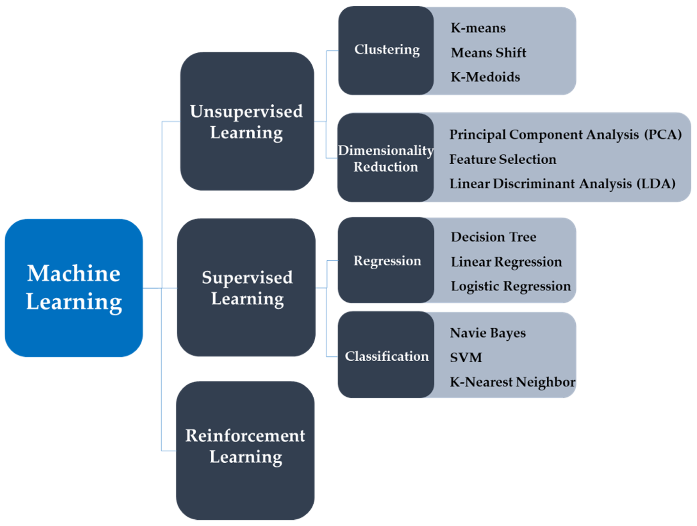
2.2. Attribute of Machine Learning Algorithms

There are many accepted versions of the definition of machine learning, but it is generally understood to mean “A computer program is said to learn from experience E with respect to some task T and some performance measure P, if its performance on T, as measured by P, improves with experience E” [29]. “Experience” can be understood as learning through data. Through this learning process, the computer modifies and adapts its behavior toward higher precision. A concept that is important to machine learning is the process of generalization. Generalization means the degree to which a program is able to predict the output of new data based on an existing machine learning model it has learned through a similar set of existing data [30]. Accordingly, it focuses on the generalization of the model’s prediction, and furthermore, making inferences on data possible.
Although a standardized classification for machine learning algorithms does not exist, as can be seen in Figure 1, depending on the data to be trained on, supervised learning, unsupervised learning, and reinforcement learning can be considered to be the main categories of classification. Of these, supervised learning is the most widely used algorithm.
The structure of supervised learning is comparatively simple and is a widely known machine learning model. It consists of input data and target data, and seeks to continuously minimize the error between the prediction value and the actual value by feeding it a large learning dataset. Such a system allows for the model to produce prediction values for new input data. The performance of the model is assessed by feeding it test data not used in the training data set [32].
Prediction techniques based on supervised learning whose variables are continuous are treated as regression problems, whereas those whose variables are categorical are treated as classification problems. It can be seen that machine learning comes in handy when a problem description that can be solved by humans but the learning dataset is too large or when a problem that can be defined mathematically is too complex for a human to be mathematically described clearly [33]. Since each analysis model has attributes, advantages, and disadvantages, this study attempted to compare predictive power using actual data. Table 2 displays attributes of the algorithm used in the study.

2.2.1. Random Forest

The random forest model was first proposed in 2001 by Leo Breiman [34]. Random forest is a method by which a singular model is generated by combining the many branches of a decision tree. RF first goes through the process of bagging, which helps improve the performance of its algorithm. Figure 2 shows the bagging process, whereby a random forest consisting of T number of decision trees is being trained on. Training data set is S 0 T for the tth decision tree through the process of bagging, and is a subset of S 0 .
An ensemble machine learning model of the random forest consists of several decision trees, pruning each branch as it traverses through in order to determine the pruning tree size. This has the effect of minimizing Equation (1) [35].
m = 1 | T | Z i R m ( y i y R ^ ) 2 α | T |
In Equation (1), | T | refers to the number of terminal nodes of tree T , R m refers to the split corresponding to the mth branch, α refers to the tuning parameter whereby α = 0 corresponds to no penalty and therefore the largest tree, and so by corollary, as α increases, the size of the tree decreases [36]. The resulting classification from each tree is voted against each other and the one with the most votes becomes the final chosen classification. Random forest works without hyper parameter tuning and has the benefit of being one of the fastest machine learning algorithms that provide prediction capabilities on regression-type problems. However, as the quantity of data increases, the speed correspondingly decreases, does not forecast over the space beyond the bounds defined by the training data, and thus suffers from an increased risk in data overfitting when the data contain a lot of noise. That being said, compared with other methods, it is shown to be superior, and much of the running research utilizes random forest for analysis purposes.

2.2.2. XGBoost

XGBoost is a model first proposed by Tianqi Chen and Carlos Guestrin in 2011 that aimed to solve the problem of overfitting in linear models or tree-based models [37]. Additionally, it has continuously been optimized in the direction of achieving stability across large data sets and faster computational time for dataset training. It is based on the CART (Classification and Regression Tree) algorithm and is a flexible model that can be accommodated for regression, classification, ranking, or otherwise a user custom objective. XGBoost runs the model up to a parameter set max depth, and when the loss function does not improve at a certain level, it proceeds with the pruning process in the opposite direction. Algorithmically, this can be described as below Algorithm 1.
Algorithm 1. Tree boosting with XGBoost [38].
  • Set f ^ ( x ) = 0 , then for each individual observation on the training set, we set the residual to the corresponding variable r i = y i
  • For the total count B , we repeat this for b = 1 , 2 , B
    • Replace the variable y with the residual r , then fit it to the decision tree with d + 1 terminal node.
    • f ^ ( x ) f ^ ( x ) + λ f ^ b ( x )
    • r i = r i λ f ^ b ( x i )
  • As a result, the boosting model has the output in the form of f ^ ( x ) = b = 1 B λ f ^ b ( x )
Within standard gradient boosting, when a negative loss occurs during the tree pruning, the process is stopped, whereas for XGBoost, a sparse away technique automatically accounts for missing data values. Additionally, it has a block structure that acts to support the parallelization of the tree structure and has the algorithmic ability to train data in a way that reflects previous data into new data to boost its performance. XGBoost prevents overfitting, and the model can be normalized with additional dimensions added to meet the user’s set optimization goal and criteria. Not only that, but cross validation is possible across each iteration of the boosting process, which has the benefit of being able to calculate the optimal boosting iteration count. Even when it comes to validation, it has an inbuilt cross validation function allowing for easy validation, and has high utility value as it is supported by various computing languages such as Python, R, Java, C++, Scala, etc. Such benefits and high performance features of this model are a reason why XGBoost is used in the field by Google, MS Azure, Alibaba, etc.

2.2.3. LSTM

LSTM is an algorithm proposed by ref. [39] and is a special form of the RNN model that is able to address the long-term dependency problem. As explained, RNN (Recurrent neural network) suffers from the reduced influence of faraway training on the current result as the sequential data quantity increases. On the other hand, LSTM has a structure known as a memory cell that is able to store the input value and so can address problems of long-term dependencies such as this. Accordingly, LSTM shows relatively good performance on jobs with long data sets [39].
All RNNs have a simplified chain-like form with a repeating neural network module. LSTM, likewise, has a similar structure, the internal repeating module is structurally different by contrast. Unlike a single level depth neural network, LSTM has four types of modules that interact with each other.
In Figure 3, we can see that the three gates have a special kind of network structure. Gates within LSTM have an important role in giving selective influence to information feeding through it at each checkpoint. This is achieved through the activation of the sigmoid function in a fully connected neural network whose structure is such that it outputs a value between 0 and 1, whereby the gate opens when the sigmoid output is 1 and passes through the information, and whereby the gate closes when the sigmoid output is 0 and no information is passed through.
The above LSTM structure can be formulated by Equations (2) and (7). σ , tanh is the hyperbolic tangent function, x t is the input, h t is the hidden variable at time t , o t is the output at time t , b is the bias, U and W are weighting factors, and i ,   o ,   f are input gates, output gates, and forget gates respectively. Each gate consists of a sigmoid neural network and multiplicative calculation layer, and at each point in time, the input gate decides whether to use the input information or not. The output gate utilizes the input and memory to determine the output and also controls the range of values for which to store into memory [41]. With the forget gate, the memory cell remembers the unit’s previous state and uses it to inform whether to apply it to the sequence of the current state. C refers to the memory cell and stores the current state of the unit [37].
i t = σ ( W i   [ h t 1 , x t ] ) + b i
f t = σ ( W f   [ h t 1 , x t ] ) + b f
C t ˜ = t a n h ( W c   [ h t 1 , x t ] ) + b c
C t = f t × C t 1 + i t × c t ˜
o t = σ ( W o   [ h t 1 , x t ] ) + b 0
h t = o t × tan ( C t )

3. Data and Methodology

3.1. Data

3.1.1. Total Energy Supply

TES (Total Energy Supply) refers to the combined final energy consumption of domestic energy production and net import, and transformation losses through energy consumption including stocks changes. Generally, TES is used when comparing the energy consumption across nation states or their consumption level [42], whereas TFC (Total Final Consumption) is used when categorizing energy consumption by sector. This paper considered TES as energy consumption for the research. TES has the following significance and utilization. Firstly, it serves as starting data for the purposes of establishing energy supply and demand plans. Coupled with energy consumption statistics, this can help support rational, energy related decision making by economic entities such as the national enterprise government. Secondly, it serves as a response indicator to changes in the domestic and foreign energy market. Through statistical analysis and forecasting of the data, a more efficient response to changes in the supply and demand of energy can be executed.

3.1.2. The Trend of Energy Consumption in Korea

The energy consumption recorded a slow growth period between 1981 and 2020 with an annualized average increase of 4.9%, which is lower than the annualized average rate of economic growth of 6.1%. Until the 1970’s, Korea used anthracite as a domestic source of energy, but following the establishing and subsequent operation of economic development started the promotion of heavy and chemical industries, resulting in an increase in oil demand from a low oil stock situation.
However, after the 1973 and 1979 first and second wave of oil shock events, respectively, an oil phase-out policy was in the works during the 1980s, which paved the way for the nascent development of bituminous coal and nuclear power generation, as well as the use of natural gas. During the early phase-out, the main energy sources were coal and petroleum, the main components of anthracite, and in the latter half of the decade, city gas, LNG, etc. started to be used. Such a trend of the primary sources of energy is shown in Figure 4.
At the current state of affairs of Korea’s energy economy is shown in Table 3. In 2018 records, the TES consumed was 282 million tons of oil equivalent (Mtoe), ranked 9th globally in energy consumption, and as the 10th largest global economy, the energy consumption size and the size of the economy are on par. Additionally, it ranked 7th globally on energy consumption, per capita power consumption at 13th, and per capita energy consumption at 15th. It ranked 7th in oil consumption, with refining capability ranked 5th; it ranked highly amongst OECD member states in 2019.
Furthermore, Korea’s energy consumption started to grow with its industrialization during the 1970s, and increased dramatically in the 1990s. The energy consumption continuously increased into the 2000s, with the 2019 supply at about 1.5 times what it was in 2001. However, the primary energy supply as a percentage of GDP is on the decline, and in Figure 5, we can see that the primary energy supply as a percentage of 2020 GDP has decreased to 5.6% of the 2001 value.
On the other hand, Korea’s energy consumption growth rate has continuously been decreasing since its financial crisis, and its reliance on oil within energy consumption has also been on the decline. In 1997, oil took 60.4% of the share, whereas in 2019, that was reduced to about 38.7%. Additionally, the growth rate of oil consumption in transport has also been on a steady decline. The per capita energy consumption of Korea is around 5.40 toe, which is 32.7% higher than the OECD average of 4.06 toe per capita. However, in the case of per capita nominal GDP, Korea is about $31,681, which is lower than the OECD average of $41,760 (2019 data). Although the income level of Korean citizens is lower than that of the OECD average, when considering the higher than average energy consumption, it speaks to the rather low energy efficiency of Korea.
With the increasing importance placed on energy security, the Korean government is pushing toward a safer, economical, and long-term strategy of energy supply. To that end, infrastructure expansion on account of safe and stable supply of natural gas, increased power plant equipment for safe power supply, and the development of the Electric Industry Restructuring for the safe supply of electricity is planned. At the same time, much consideration is being placed on the development and increased utilization of alternative sources of energy and their appropriate proportioning with traditional sources of energy for more efficient use of energy.
Given this context, the precise calculation and forecasting of energy demand are deeply intertwined with the energy economy and development of Korea and as such plays a crucial role in the energy policy of the country. The aim of this research was to utilize machine learning techniques to provide a quicker, more precise energy demand forecasting model.

3.1.3. COVID-19 Crisis on Global Energy Supply and Demand

Coronavirus disease 2019 (henceforth referred to as COVID-19) has spread rapidly around the world since it was first discovered in December 2019, and the World Health Organization (WHO) declared COVID-19 as a pandemic in March 2020. As the number of confirmed cases around the world exploded due to the COVID-19 pandemic, border blockades and full lockdowns were implemented by countries [47]. These quarantine measures have led to all-round changes from economic activities to lifestyle. The IMF analyzes the global economic slowdown caused by the COVID-19 pandemic as the most serious since the Great Depression [48]. In order to prevent the spread of COVID-19, Korea implemented social distancing step by step instead of blockade measures.
The economic downturn and changes in people’s lifestyles caused by the COVID-19 pandemic had a serious impact on the energy market. The IEA predicted that COVID-19 would act as the biggest shock since World War II, plunging global energy consumption and reducing greenhouse gas emissions by nearly 8% [49]. As industrial production activities shrink and people’s lifestyles change due to the spread of COVID-19, not only electricity but also energy consumption in Korea decreased in 2020. The TES, which had been on the rise, showed a decreasing trend for two consecutive years for the first time ever in 2019 and 2020.
In 2020, Korea’s gross domestic product decreased by 1.0% compared with the previous year, and total energy consumption was counted at 290.8 million toes, down 4.0% from the previous year. Electricity sales also fell 2.2% year on year [50]. In predicting the trend of the energy market, this study attempted to increase the effectiveness of the predictive model by dividing it into the pre COVID-19 period and the subsequent period.

3.1.4. Independent Variables

This research used the energy demand data between the period of January 1996 and June 2021 for analysis. In much of existing empirical research, reduced form models that included as many possible variables did not perform significantly better than reduced form models that had important variables selected for regression analysis [51]. Additionally, the dynamic interplay between past energy usage, economy, population statistics, climate, energy pricing, and other related variables are generally considered a basis for energy consumption computational modelling.
As such, in this research, considering the frequency of use of various explanatory variables used in existing literature, GDP, population, temperature, oil prices, and independent variables of power generation were used for forecasting. The basic statistics of each variable are shown in Table 4.
Given that the data for Gross Domestic Product (GDP) produced on a quarterly basis needs to be converted into monthly data, the index of Manufacturing Production, which has identical correlation to the GDP, is used as an indicator in its stead. Korea imports 70–80% of the total crude oil volume from the Middle East, and as such, given that it is mainly influenced by Dubai Crude out of the three major oil suppliers (WTI, Brent Crude, Dubai Crude), it was used as the oil price variable. All independent variables have a high correlation with the dependent variables (domestic, non-domestic, total consumption), and they are widely used in predictive models [52].

3.2. Methodology

In this research, three machine learning algorithms were used and compared on the basis of their training accuracy. The analysis period was divided into a stable market period and an unstable market period. The reason for dividing the period is that the predictive ability of the model may vary depending on the market situation.
Following this, Period 1 of “January 1997 to December 2013” was set as training data, January 2014 to December 2015 as valid data, and the stable uptrend period of January 2016 to December 2017 as the test data. On the other hand, 2019 saw the first downtrend in energy consumption after the financial crisis of 1998, the primary reason for which is attributed to the spread of COVID-19 and the wild fluctuations in the economy that followed, coupled with the uncertainty in the supply of energy became all too apparent [53]. Additionally, power generation fueled by coal and gas was reduced due to the economic slowdown in manufacturing production, and the energy consumption in the infrastructure sector decreased by 2.0% compared with the previous year (2018) of which Heating Degree Day (HDD) and Cooling Degree Day (CDD) dramatically declined on account of the overlap of heat waves and cold waves [53].
Following this, Period 2 uses “January 1997 to June 2017” as training data, “July 2017 to June 2019” as valid data, the period which saw a dramatic shift in the energy market due to the shockwave following COVID-19 etc. of “July 2019 to June 2021” as the test data, and provides separate models to demonstrate and cross analyze their respective predictive performance according to the market situation. The machine learning model uses the statistics package from python for empirical analysis.

3.3. Evaluating Forecast Accuracy

To be able to select the model that is best able to predict results on new input data is the most important yet most difficult job [35]. Within this research, the most widely adopted reliability analysis indicator in the context of prediction driven models of Root Mean Squared Error (RMSE) and Mean Absolute Percentage Error (MAPE) was used. The equation to calculate the RMSE is shown in Equation (8), while the equation to calculate the MAPE is shown in Equation (9).
RMSE = i = 1 n ( x 1 , i x 2 , i ) 2 n    
MAPE = 1 n i = 1 n | x 1 , i x 2 , i x 1 , i | × 100  
In the above equation, x 1 , i is the actual observation, whereas x 2 , i is the estimated value calculated by the model.

4. Korea Energy Consumption Forecasting Model

4.1. Random Forest Model

In the Random Forest model, the hyperparameter tree estimator is changed, max depth changed, and the hyperparameter whose final RMSE value is minimized is selected as the final model. In Period 1 and Period 2, in order to find the RF model whose RMSE value is minimal, repeated training was conducted. One thing to note is that since the RF model is not a time series model, through the process of making the months into dummy variables for the purposes of creating a variety of tree classifications, pitchers were added.
Additionally, the min max scaler was used to improve performance with the input boundary values changed to be between −1 and +1. The upper bound for the tree estimator was set to 500, while the lower bound was initialized to 50. Given the features of the max depth data, the upper bound was set to 7 and the lower bound set to 3. Through repeated model training, the model with the minimal RMSE was chosen as the final Random Forest model. In Period 1, the tree with estimator 300, max depth 5 minimized RMSE the most, while for Period 2, the tree with estimator 500, max depth 6 minimized the RMSE the most. Figure 6 is a comparison graph of actual and predicted values for energy consumption.

4.2. XGBoost Model

In the XGBoost model, the hyperparameter tree estimator was changed, and with max depth, learning rate also changed, with the hyperparameter whose final value of RMSE was minimized being selected as the final model.
For Period 1 and Period 2, repeated training was conducted with the XGBoost model in order to find the minimum RMSE value. One thing to note is that since the XGBoost model is not a time series model, through the process of making the months into dummy variables for the purposes of creating a variety of tree classifications, pitchers were added. Additionally, the min max scaler was used to improve performance with the input boundary values changed to be between −1 and +1. The upper bound for the tree estimator was set to 500 while the lower bound was initialized to 100. Additionally, according to the XGBoost model’s learning rate, the model’s resultant value can change, and so, the learning rate was set to 0.001, 0.01, 0.05, and 0.1.
Through repeated model training, the model with the minimal RMSE was chosen as the final Random Forest model. In the event of an equivalent minimum value, the model whose learning process terminated sooner was chosen as the final model. This is because as the size of the data increases, and depending on the features of the data, the model’s learning time can change, and those whose learning times were quicker were considered to be superior.
In Period 1, the tree with estimator 100, max depth 3, learning rate 0.05 minimized RMSE the most, while for Period 2, the tree with estimator 100, max depth 7, learning rate 0.1 minimized the RMSE the most. A parameter was chosen for each period, and these were chosen to be the optimal XGBoost model for that period. Figure 7 is a comparison graph of actual and predicted values for energy consumption.

4.3. LSTM Model

As was with the RF model and the XGBoost model, the ANN model LSTM utilized the same data. In the case of artificial neural networks, the approach use stacked hidden layers, and depending on the Epoch, the data results may vary. In order to analyze the earlier data, the LSTM model used the Keras deep learning library from the Python language. Furthermore, the LSTM uses the Keras deep learning library with a default activation function that outputs a value between −1 and 1 via the hyperbolic tangent function. As such, by using the min max scaler, the input values are similarly changed to a measure between −1 and 1. The behavior of the LSTM model can change depending on the optimizer and activation function used. As such, since tuning the parameters affects the resulting value, suitable values for the parameters were obtained through a grid search approach within a set boundary while the overall structure remained fixed.
In this research, the ReLU activation [54,55] was used as it was, proven to be the most effective. Furthermore, in order to reduce overfitting and improve the performance of the model, the dropout and recurrent dropout settings were each set to 0.1 [56]. The epochs were set to 100, with an early stopping function with a patience setting of 10 put in place in order to make sure the loss function output did not increase during the training. Next, setting the number of units as 8, 16, 32, the learning rate as 0.01, 0.05, 0.1, and batch size as 16, 32, 48 as variables, all possible combinations were attempted. The result of which was that out of the 26 possible combinations, for Period 1, when the parameters were unit 16, learning 0.001, batch size 16, the RMSE was minimized, and for Period 2, when the parameters were unit 16, learning rate 0.05, batch size 32, the RMSE was similarly minimized. The selected parameters were used to build the model for each time period. Figure 8 is a comparison graph of actual and predicted values for energy consumption.

5. Results and Discussion

The Random forest, XGBoost, and LSTM model were implemented using the package Scikit learn [18,57]. The model with the lowest RMSE value was selected as the final model. Table 5 shows a comparison of the RMSE values of the machine learning model’s test data for Period 1 and Period 2. The parameters that yielded the lowest RMSE value for the LSTM model for Period 1 were unit 16, learning rate 0.001, and batch size 16. The parameters that yielded the lowest RMSE value for the Random Forest model for Period 2 were tree estimator 500 and max depth 6.
For the comparison of prediction, there are other predicted values on Table 6. It shows the predicted value not only machine learning algorithms but also ARIMA and ARDL. The ARIMA, which is one of the most popular models for time series forecasting analysis, originated from the autoregressive model (AR), the moving average model (MA), and the combination of the AR and MA, the ARMA models [58,59,60,61,62,63,64]. The Korea Energy Economics Institute (KEEI) announces the outlook using the Autoregressive Distributed Lag (ARDL) model for energy supply and demand twice a year [65].
In Table 6, ARIMA and ARDL predictions [66,67] are closer to the actual values in 2017 and 2018. Meanwhile, the predicted value with higher accuracy can be achieved through the proposed machine learning model in 2019, 2020, and 2021. It demonstrated that traditional econometric approaches may outperform machine learning when there is less unknown irregularity in the time series, but machine learning can work better with unexpected irregular time series data.
Figure 9, Figure 10 and Figure 11 show the machine learning predicted value against the actual value and the optimal model’s predicted value for each time period in each graph for ease of comparison. In addition, it can visually be observed that there was difference in the forecasting capability across all machine learning models through prediction error. However, though the models tracked the decline rather well, the predicted value strayed a noticeable amount in tracking the post rebound rise. Overall, In Period 1, LSTM displayed superior results by tracking similar trend intervals. The optimal model of Period 2 being Random Forest also yielded near identical prediction values to the actual value.
When observing the results of the machine learning approaches, the stable Period 1 prior to COVID-19 without the large market shock was best predicted by the LSTM model out of all the machine learning models. On the other hand, Period 2, with the large shock caused by COVID-19, economic stagnation due to the resulting recession, sudden decrease in HDD and CDD, and the overall volatility in the energy market, had the most effective predictive potential by RF out of all the machine learning models.

6. Conclusions

The accurate prediction of total energy consumption is crucial in implementing effective energy policy. As mentioned earlier, Korea has a high reliance on energy import, and when such an energy dependence rate is high, accurate prediction of the energy consumption (which is directly related to the energy efficiency indicator) is important. This is because, through this, energy-related problems can be effectively addressed along with planning the stable growth of the economy [68].
However, due to Korea’s rapid economic growth and the associated increased demand in power and oil, using socio-economic indicators to develop forecasting tools is a challenging feat. In predicting the energy demand, this research used the total energy consumption and highly correlated variables (oil price, population, power generation, index of manufacturing production, temperature) to confirm the suitability and usability of machine learning forecasting. Additionally, in predicting the total energy consumption, this research separated the time period of analysis into the comparatively stable market period before the COVID-19 pandemic, and the subsequent unstable market.
To summarize the results of the research, firstly, Period 1 was most accurately predicted by the LSTM model. Secondly, the RF model tended to yield the lowest RMSE and MAPE in period 2. The following points are implications derived from the results of the study. LSTM, which could take periodic movements into account, showed meaningful predictive performance relative to the different machine learning methods when the market trend was consistent. LSTM has many advantages over other feedforward and recurrent NNs in the modeling of time series [69]. However, in nonlinear system modeling, normal LSTM does not work well [70]. When the market behavior changed from one trend to another, RF, with its nonlinear modelling capability, displayed the most effective predictive results [71].
The main contributions of this study are as follows. We showed the applicability of machine learning to forecast energy consumption and also demonstrated that traditional econometric approaches may outperform machine learning when there is less unknown irregularity in the time series, but machine learning can work better with unexpected irregular time series data.
This study has the following aspects of interdisciplinary and practical application. The predictive power of machine learning in the energy market was verified using actual data. In practice, this study can be expanded to contribute to enhancing the reliability of energy supply and demand data. As such, energy-related companies and governments can respond appropriately to changes in energy consumption using this forecasting model.
The limitations and the future research direction as a result of this research are as follows. Firstly, the actual accuracy of prediction and analysis of the model can change depending on the analysis data and variable settings, and as such, it is hard to conclusively state that a specific approach is superior across all time periods, and further research is required on this matter [72]. To make up for this, a separate time period covering post COVID-19 was included for the comparative prediction, but it is a separate matter to say whether the results presented here will also apply to future data. Secondly, much of artificial intelligence is plagued by the “black box problem.” While we may know the inputs and outputs of a model, in many cases, we cannot explain the prediction of a model [73,74,75].
Therefore, in future work, further study is required by means of combining Explainable AI (XAI) models and combining machine and econometrics methods for interpretable analytics.

Author Contributions

Conceptualization, S.-Y.S.; Investigation, S.-Y.S.; Methodology, S.-Y.S. and H.-G.W.; Supervision, H.-G.W.; Validation, S.-Y.S.; Visualization, S.-Y.S.; Writing—original draft, S.-Y.S.; Writing—review & editing, S.-Y.S. and H.-G.W. All authors have read and agreed to the published version of the manuscript.

Funding

This research received no external funding.

Institutional Review Board Statement

Not applicable.

Informed Consent Statement

Not applicable.

Data Availability Statement

Data were obtained from Korea Energy Economics Institute and are available with the permission of Korea Energy Economics Institute.

Conflicts of Interest

The authors declare no conflict of interest.

References

  1. Ha, Y.H.; Byrne, J. The rise and fall of green growth: Korea’s energy sector experiment and its lessons for sustainable energy policy. Wiley Interdiscip. Rev. Energy Environ. 2019, 8, e335. [Google Scholar] [CrossRef] [Green Version]
  2. Geem, Z.W.; Roper, W.E. Energy demand estimation of South Korea using artificial neural network. Energy Policy 2009, 37, 4049–4054. [Google Scholar] [CrossRef]
  3. Suganthi, L.; Samuel, A.A. Energy models for demand forecasting—A review. Renew. Sustain. Energy Rev. 2012, 16, 1223–1240. [Google Scholar] [CrossRef]
  4. Zhu, Q.; Guo, Y.; Feng, G. Household energy consumption in China: Forecasting with BVAR model up to 2015. In Proceedings of the 2012 Fifth International Joint Conference on Computational Sciences and Optimization, Harbin, China, 23–26 June 2012; pp. 654–659. [Google Scholar]
  5. Herrera, G.P.; Constantino, M.; Tabak, B.M.; Pistori, H.; Su, J.-J.; Naranpanawa, A. Long-term forecast of energy commodities price using machine learning. Energy 2019, 179, 214–221. [Google Scholar] [CrossRef]
  6. Chavez, S.G.; Bernat, J.X.; Coalla, H.L. Forecasting of energy production and consumption in Asturias (northern Spain). Energy 1999, 24, 183–198. [Google Scholar] [CrossRef]
  7. Ceylan, H.; Ozturk, H.K. Estimating energy demand of Turkey based on economic indicators using genetic algorithm approach. Energy Convers. Manag. 2004, 45, 2525–2537. [Google Scholar] [CrossRef]
  8. Crompton, P.; Wu, Y. Energy consumption in China: Past trends and future directions. Energy Econ. 2005, 27, 195–208. [Google Scholar] [CrossRef]
  9. Mohamed, Z.; Bodger, P. Forecasting electricity consumption in New Zealand using economic and demographic variables. Energy 2005, 30, 1833–1843. [Google Scholar] [CrossRef] [Green Version]
  10. Pao, H.-T. Comparing linear and nonlinear forecasts for Taiwan’s electricity consumption. Energy 2006, 31, 2129–2141. [Google Scholar] [CrossRef]
  11. Toksarı, M.D. Ant colony optimization approach to estimate energy demand of Turkey. Energy Policy 2007, 35, 3984–3990. [Google Scholar] [CrossRef]
  12. Ekonomou, L. Greek long-term energy consumption prediction using artificial neural networks. Energy 2010, 35, 512–517. [Google Scholar] [CrossRef] [Green Version]
  13. Lee, Y.-S.; Tong, L.-I. Forecasting energy consumption using a grey model improved by incorporating genetic programming. Energy Convers. Manag. 2011, 52, 147–152. [Google Scholar] [CrossRef]
  14. Ardakani, F.; Ardehali, M. Long-term electrical energy consumption forecasting for developing and developed economies based on different optimized models and historical data types. Energy 2014, 65, 452–461. [Google Scholar] [CrossRef]
  15. Barak, S.; Sadegh, S.S. Forecasting energy consumption using ensemble ARIMA–ANFIS hybrid algorithm. Int. J. Electr. Power Energy Syst. 2016, 82, 92–104. [Google Scholar] [CrossRef] [Green Version]
  16. Kim, Y.; Park, H. Modeling and Predicting South Korea’s Daily Electric Demand Using DNN and LSTM. J. Clim. Res. 2021, 12, 241–253. [Google Scholar]
  17. Sözen, A.; Arcaklioğlu, E.; Özkaymak, M. Turkey’s net energy consumption. Appl. Energy 2005, 81, 209–221. [Google Scholar] [CrossRef]
  18. Ediger, V.Ş.; Akar, S. ARIMA forecasting of primary energy demand by fuel in Turkey. Energy Policy 2007, 35, 1701–1708. [Google Scholar] [CrossRef]
  19. Bianco, V.; Manca, O.; Nardini, S. Electricity consumption forecasting in Italy using linear regression models. Energy 2009, 34, 1413–1421. [Google Scholar] [CrossRef]
  20. Kankal, M.; Akpınar, A.; Kömürcü, M.İ.; Özşahin, T.Ş. Modeling and forecasting of Turkey’s energy consumption using socio-economic and demographic variables. Appl. Energy 2011, 88, 1927–1939. [Google Scholar] [CrossRef]
  21. Park, K.-R.; Jung, J.-Y.; Ahn, W.-Y.; Chung, Y.-S. A study on energy consumption predictive modeling using public data. In Proceedings of the Korean Society of Computer Information Conference, Seoul, Korea, 10 July 2012; pp. 329–330. [Google Scholar]
  22. Xiong, P.-P.; Dang, Y.-G.; Yao, T.-X.; Wang, Z.-X. Optimal modeling and forecasting of the energy consumption and production in China. Energy 2014, 77, 623–634. [Google Scholar] [CrossRef]
  23. Yuan, C.; Liu, S.; Fang, Z. Comparison of China’s primary energy consumption forecasting by using ARIMA (the autoregressive integrated moving average) model and GM (1, 1) model. Energy 2016, 100, 384–390. [Google Scholar] [CrossRef]
  24. Wang, Q.; Li, S.; Li, R. Forecasting energy demand in China and India: Using single-linear, hybrid-linear, and non-linear time series forecast techniques. Energy 2018, 161, 821–831. [Google Scholar] [CrossRef]
  25. Oh, W.; Lee, K. Causal relationship between energy consumption and GDP revisited: The case of Korea 1970–1999. Energy Econ. 2004, 26, 51–59. [Google Scholar] [CrossRef]
  26. Shin, J.; Yang, H.; Kim, C. The relationship between climate and energy consumption: The case of South Korea. Energy Sources Part A: Recovery Util. Environ. Eff. 2019, 1–16. [Google Scholar] [CrossRef]
  27. Lee, S.; Jung, S.; Lee, J. Prediction model based on an artificial neural network for user-based building energy consumption in South Korea. Energies 2019, 12, 608. [Google Scholar] [CrossRef] [Green Version]
  28. Moon, J.; Kim, Y.; Son, M.; Hwang, E. Hybrid short-term load forecasting scheme using random forest and multilayer perceptron. Energies 2018, 11, 3283. [Google Scholar] [CrossRef] [Green Version]
  29. Mitchell, T.M.; Carbonell, J.G.; Michalski, R.S. Machine Learning: A Guide to Current Research; Springer Science & Business Media: Berlin/Heidelberg, Germany, 1986. [Google Scholar]
  30. Domingos, P. A few useful things to know about machine learning. CACM 2012, 55, 78–87. [Google Scholar] [CrossRef] [Green Version]
  31. Berry, M.W.; Mohamed, A.; Yap, B.W. (Eds.) Supervised and Unsupervised Learning for Data Science; Springer Nature: Berlin/Heidelberg, Germany, 2019. [Google Scholar]
  32. Vieira, S.; Lopez Pinaya, W.H.; Garcia-Dias, R.; Mechelli, A. Chapter 9—Deep neural networks. In Machine Learning; Mechelli, A., Vieira, S., Eds.; Academic Press: Cambridge, MA, USA, 2020; pp. 157–172. [Google Scholar]
  33. Mohammed, M.; Khan, M.B.; Bashier, E.B.M. Machine Learning: Algorithms and Applications, 1st ed.; CRC Press: Boca Raton, FL, USA, 2016. [Google Scholar]
  34. Breiman, L. Random forests. Mach. Learn. 2001, 45, 5–32. [Google Scholar] [CrossRef] [Green Version]
  35. James, G.; Witten, D.; Hastie, T.; Tibshirani, R. An Introduction to Statistical Learning; Springer: New York, NY, USA, 2013; Volume 103. [Google Scholar]
  36. Lee, C. Estimating Single-Family House Prices Using Non-Parametric Spatial Models and an Ensemble Learning Approach. Ph.D. Thesis, Seoul National University, Seoul, Korea, 2015. [Google Scholar]
  37. Chen, T.; Guestrin, C. Xgboost: A scalable tree boosting system. In Proceedings of the 22nd ACM SIGKDD International Conference on Knowledge Discovery and Data Mining, San Francisco, CA, USA, 13–17 August 2016; pp. 785–794. [Google Scholar]
  38. Friedman, J.H. Stochastic gradient boosting. Comput. Stat. Data Anal. 2002, 38, 367–378. [Google Scholar] [CrossRef]
  39. Hochreiter, S.; Schmidhuber, J. Long short-term memory. Neural Comput. 1997, 9, 1735–1780. [Google Scholar] [CrossRef]
  40. Olah, C. Understanding LSTM Networks. 2015. Available online: http://colah.github.io/posts/2015-08-Understanding-LSTMs/ (accessed on 18 April 2022).
  41. Brownlee, J. Introduction to Time Series Forecasting with Python; Machine Learning Mastery: San Francisco, CA, USA, 2019. [Google Scholar]
  42. Energy Agency (IEA). Energy Statistics Manual; IEA: Paris, France, 2004. [Google Scholar]
  43. Energy Agency (IEA). World Energy Balances; IEA: Paris, France, 2020. [Google Scholar]
  44. BP. Statistical Review of World Energy, 69th ed.; BP: London, UK, 2020. [Google Scholar]
  45. Korea Energy Economics Institute. Monthly Energy Statistics (2021.12); Korea Energy Economics Institute: Ulsan, Korea, 2021; Volume 37-12, p. 7. [Google Scholar]
  46. Korea Energy Economics Institute. Yearbook of Energy Statistics; Korea Energy Economics Institute: Ulsan, Korea, 2021; Volume 606, pp. 20–21. [Google Scholar]
  47. Bahmanyar, A.; Estebsari, A.; Ernst, D. The impact of different COVID-19 containment measures on electricity consumption in Europe. Energy Res. Soc. Sci. 2020, 68, 101683. [Google Scholar] [CrossRef] [PubMed]
  48. Gopinath, G. The great lockdown: Worst economic downturn since the great depression. IMF Blog 2020, 14, 2020. [Google Scholar]
  49. IEA Ukraine. Global Energy Review 2020. Ukraine, 2020. Available online: https://www.iea.org/countries/ukraine (accessed on 10 September 2020).
  50. Korea Energy Economics Institute. Monthly Energy Statistics (2021.8); Korea Energy Economics Institute: Ulsan, Korea, 2021; Volume 37-08, p. 7. [Google Scholar]
  51. Gürkaynak, R.S.; Kısacıkoğlu, B.; Rossi, B. Do DSGE Models Forecast More Accurately Out-Of-Sample than VAR Models? In VAR Models in Macroeconomics—New Developments and Applications: Essays in Honor of Christopher A. Sims; Advances in Econometrics; Emerald Group Publishing Limited: Bingley, UK, 2013; Volume 32, pp. 27–79. [Google Scholar]
  52. Makridakis, S.; Wheelwright, S.C.; Hyndman, R.J. Forecasting Methods and Applications; John Wiley & Sons: Hoboken, NJ, USA, 2008. [Google Scholar]
  53. Korea Energy Economics Institute. Korea Mid-Term Energy Demand Outlook (2020–2025); Korea Energy Economics Institute: Ulsan, Korea, 2021. [Google Scholar]
  54. Nair, V.; Hinton, G.E. Rectified linear units improve restricted boltzmann machines. In Proceedings of the 27th International Conference on Machine Learning, Haifa, Israel, 21–24 June 2010. [Google Scholar]
  55. Kingma, D.P.; Ba, J. Adam: A method for stochastic optimization. arXiv 2014, arXiv:1412.6980. [Google Scholar]
  56. Srivastava, N. Improving Neural Networks with Dropout. Master’s Thesis, University of Toronto, Toronto, ON, Canada, 2013. [Google Scholar]
  57. Pedregosa, F.; Varoquaux, G.; Gramfort, A.; Michel, V.; Thirion, B.; Grisel, O.; Blondel, M.; Prettenhofer, P.; Weiss, R.; Dubourg, V.; et al. Scikit-learn: Machine learning in Python. J. Mach. Learn. Res. 2011, 12, 2825–2830. [Google Scholar]
  58. Blanchard, M.; Desrochers, G. Generation of autocorrelated wind speeds for wind energy conversion system studies. Solar Energy 1984, 33, 571–579. [Google Scholar] [CrossRef]
  59. Brown, B.G.; Katz, R.W.; Murphy, A.H. Time series models to simulate and forecast wind speed and wind power. J. Appl. Meteorol. Climatol. 1984, 23, 1184–1195. [Google Scholar] [CrossRef]
  60. Kamal, L.; Jafri, Y.Z. Time series models to simulate and forecast hourly averaged wind speed in Quetta, Pakistan. Solar Energy 1997, 61, 23–32. [Google Scholar] [CrossRef]
  61. Ho, S.L.; Xie, M. The use of ARIMA models for reliability forecasting and analysis. Comput. Ind. Eng. 1998, 35, 213–216. [Google Scholar] [CrossRef]
  62. Saab, S.; Badr, E.; Nasr, G. Univariate modeling and forecasting of energy consumption: The case of electricity in Lebanon. Energy 2001, 26, 1–14. [Google Scholar] [CrossRef]
  63. Zhang, G.P. Time series forecasting using a hybrid ARIMA and neural network model. Neurocomputing 2003, 50, 159–175. [Google Scholar] [CrossRef]
  64. Ho, S.L.; Xie, M.; Goh, T.N. A comparative study of neural network and Box-Jenkins ARIMA modeling in time series prediction. Comput. Ind. Eng. 2002, 42, 371–375. [Google Scholar] [CrossRef]
  65. Korea Energy Economics Institute. Korea Energy Demand Outlook; Korea Energy Economics Institute: Ulsan, Korea, 2019; Volume 21, pp. 55–56. [Google Scholar]
  66. Korea Energy Economics Institute. Korea Mid-Term Energy Demand Outlook (2016~2021); Korea Energy Economics Institute: Ulsan, Korea, 2017; p. 93. [Google Scholar]
  67. Gonzalez, J.; Yu, W. Non-linear system modeling using LSTM neural networks. IFAC-Pap. 2018, 51, 485–489. [Google Scholar] [CrossRef]
  68. Han, J.G. The Politics of Expertise in Korean Energy Policy: The Sociology of Energy Modelling (Publication No.000864823). Ph.D. Thesis, College of Social Sciences, Kookmin University, Seoul, Korea, 2015. [Google Scholar]
  69. Korea Energy Economics Institute. Korea Mid-Term Energy Demand Outlook (2017~2022); Korea Energy Economics Institute: Ulsan, Korea, 2018; p. 97. [Google Scholar]
  70. Zeng, Y.-R.; Zeng, Y.; Choi, B.; Wang, L. Multifactor-influenced energy consumption forecasting using enhanced back-propagation neural network. Energy 2017, 127, 381–396. [Google Scholar] [CrossRef]
  71. Krauss, C.; Do, X.A.; Huck, N. Deep neural networks, gradient-boosted trees, random forests: Statistical arbitrage on the S&P 500. Eur. J. Oper. Res. 2017, 259, 689–702. [Google Scholar]
  72. Armstrong, J.S.; Collopy, F. Error measures for generalizing about forecasting methods: Empirical comparisons. Int. J. Forecast. 1992, 8, 69–80. [Google Scholar] [CrossRef] [Green Version]
  73. Mullainathan, S.; Spiess, J. Machine learning: An applied econometric approach. J. Econ. Perspect. 2017, 31, 87–106. [Google Scholar] [CrossRef] [Green Version]
  74. Lipton, Z.C. The mythos of model interpretability: In machine learning, the concept of interpretability is both important and slippery. Queue 2018, 16, 31–57. [Google Scholar] [CrossRef]
  75. Kauffman, R.J.; Kim, K.; Lee, S.Y.T.; Hoang, A.P.; Ren, J. Combining machine-based and econometrics methods for policy analytics insights. Electron. Commer. Res. Appl. 2017, 25, 115–140. [Google Scholar] [CrossRef]
Figure 1. Types of machine learning algorithms [31].
Energies 15 04880 g001
Figure 2. Typical architectures of bagging.
Energies 15 04880 g002
Figure 3. LSTM cell structure [40].
Energies 15 04880 g003
Figure 4. Primary sources of energy [45].
Energies 15 04880 g004
Figure 5. Energy consumption per GDP [45,46].
Energies 15 04880 g005
Figure 6. Random forest forecasting.
Energies 15 04880 g006
Figure 7. XGBoost forecasting.
Energies 15 04880 g007
Figure 8. LSTM Forecasting.
Energies 15 04880 g008
Figure 9. Random forest model comparison by period with prediction error.
Energies 15 04880 g009
Figure 10. XGBoost model comparison by period with prediction error.
Energies 15 04880 g010
Figure 11. LSTM model comparison by period with prediction error.
Energies 15 04880 g011
Table 1. List of reviewed articles.
AuthorsMethod UsedForecasting ScopeForecast Energy TypeEnergy Market
Chav, Bernat and Coalla [6]ARIMAMonthlyEnergy production and consumptionAsturias (northern Spain)
Ceylan and Ozturk [7]GAEDMAnnualEnergy demandTurkey
Crompton and Wu [8]Bayesian vector autoregressionAnnualEnergy consumptionChina
Mohamed and Bodger [9]Multiple linear regressionAnnualElectricity consumptionNew Zealand
Sözen, et al. [17]ANNAnnualNet energy consumptionTurkey
Pao [10]ANN, linear and non-linear statistical modelsAnnualElectricity consumptionTaiwan
Ediger and Akar [18]ARIMA, SARIMAAnnualPrimary energy demand by fuelTurkey
Toksarı [11]ACO (Ant Colony Optimization)AnnualEnergy demandTurkey
Bianco, et al. [19]Linear regressionAnnualElectricity consumptionItaly
Geem and Roper [3]ANNAnnualEnergy demandKorea
Ekonomou [11]ANNAnnualEnergy consumptionGreece
Kankal, et al. [20]ANNAnnualEnergy consumptionTurkey
Zhu, Guo and Feng [4]BVARAnnualHousehold energy consumptionChina
Park, et al. [21]Markov ProcessMonthlyEnergy consumptionKorea
Xiong, et al. [22]GM (1, 1)AnnualEnergy production and consumptionChina
Ardakani and Ardehali [13]Multivariable regression, ANNAnnualElectrical energy consumptionIran, United States
Yuan, et al. [23]GM (1, 1) and ARIMAAnnualEnergy consumptionChina
Wang et al. [24]DNN, ANNAnnualEnergy demandChina, India
Kim, Y. and Park, H. [15]DNN, LSTMShort term (Daily)Electric DemandKorea
Table 2. Attributes of the algorithms.
AlgorithmsDescriptionProsCons
Random Forest
  • Operate by constructing a multitude of decision trees at training time
  • Prevent overfitting
  • Low interpretability
  • Output the class that is the mode of the classification or regression of the individual trees
  • Good with very large data set
  • Correct for decision trees’ habit of overfitting to their training set
  • No transformation needed
  • Less accurate than boosted tree models
  • Robust against outliers
XGBoost
  • An advanced implementation of gradient boosting algorithm
  • Use regularization to reduce overfitting
  • Susceptible to outliers
  • Use a more regularized model formalization to control over fitting, which gives it better performance
  • Support parallel processing
  • Lack of interpretability and higher complexity
  • Make splits up to the max depth specified and then start pruning the tree backward and remove splits beyond which there is no positive gain
  • Harder to tune parameters than other models
  • Built-in Cross Validation
  • Slow to train or score
LSTM
  • Variant of RNNs that introduce a number of special, internal gates
  • Introduces many more internal parameters which must be learned—Flexible
  • Introduces many more internal parameters which must be learned—Time consuming
  • Internal gates help with the problem of learning relationships between both long and short sequences in data
Table 3. Country comparison of energy consumption [43] (1) [44] (2).
RankingTotal Energy
Supply (TES) (1)
(Million Toe)
Oil
Consumption (2)
(Million Tonnes)
Oil Refinery
Capacity (2)
(Thousand
Barrels Daily)
Electricity
Consumption (1)
(TWh)
TES/Population (1)
(Toe per Capita)
Electricity
Consumption/Population (1)
(kWh per Capita)
1ChinaUnited StatesUnited StatesChinaIcelandIceland
321184218,974688017.454,605
2United StatesChinaChinaUnited StatesQatarNorway
223165016,199419415.624,047
3IndiaIndiaRussiaIndiaTrinidad and TobagoBahrain
9192426721130912.2518,618
4RussiaJapanIndiaRussiaBahrainQatar
75917450089979.0816,580
5JapanSaudi ArabiaKoreaJapanBruneiFinland
42615933939558.6215,804
6GermanyRussiaJapanCanadaCuraçaoCanada
30215133435728.2915,438
7CanadaKoreaSaudi ArabiaKoreaKuwaitKuwait
29812028355638.2215,402
8BrazilBrazilIranGermanyCanadaLuxembourg
28711024055598.0313,476
9KoreaGermanyBrazilBrazilUnited Arab EmiratesSweden
28210722905537.0213,331
10IranCanadaGermanyFranceKorea (15th)Korea (13th)
26610320854745.4711,082
World14,2824445101,34019,2781.883260
(1) Energy Agency (IEA). World Energy Balances; IEA: Paris, France, 2020. (2) BP. Statistical Review of World Energy, 69th ed.; BP: London, UK, 2020.
Table 4. Basic statistics of independent variables.
VariableUnitAverageMaxMinMedianStandard Deviation
Oil Prices (Dubai)$/bbl.55.6131.310.153.730.8
Index of Manufacturing Production2015 = 10078.8118.831.084.025.0
Population1000 Persons49,224.151,821.745,953.649,307.81817.4
Average Temperature°C12.928.8−7.214.09.9
Power GenerationGWh35,079.653,394.216,228.036,458.510,093.8
Table 5. Performance of the models by period.
Period 1RFXGBLSTM
RMSE0.0610.0740.052
MAPE0.0700.0960.079
ParameterEstimator: 300Estimator: 100Activation: Relu
Learning rate: 0.05Unit: 16
Max Depth: 5Max depth: 3Learning rate: 0.001
Batch: 16
Period 2RFXGBLSTM
RMSE0.0400.0500.080
MAPE0.0470.0530.062
ParameterEstimator: 500Estimator: 100Activation: Relu
Learning rate: 0.1Unit: 16
Max Depth: 6Max depth: 7Learning rate: 0.05
Batch: 32
Table 6. Predicted value of ML, ARIMA, and ARDL. Unit: 1000 toe.
YearTrue ValuePredicted Value
Machine LearningARIMAARDL
2017302,490297,017299,485302,500
2018307,557304,200311,663308,800
2019303,092301,897318,726314,000
2020292,076299,244311,664320,300
The first half of 2021150,188150,277158,250162,450
Publisher’s Note: MDPI stays neutral with regard to jurisdictional claims in published maps and institutional affiliations.

