1. Introduction
In recent years, scientific discoveries and technological advances have meant that the terraformation of Mars can be considered not just in terms of science fiction but also of applied science. Mars satellite missions, both in the past (the Mariner program in the 1960s and the Viking program in the 1970s) and modern (Mars Odyssey 2001, Mars Express 2003, Mars Reconnaissance Orbiter 2005, Mangalyaan 2013, MAVEN 2013, ExoMars Trace Gas Orbiter 2016, InSight 2018, Mars 2020 Perseverance 2021), have significantly helped expand our knowledge about the Red Planet. The current challenges facing science are the preparation of a manned mission and the answer to whether it is possible to anthropogenically transform the atmospheric conditions on Mars and make them resemble Earth’s conditions, and if so, over what time perspective. The main challenges for the terraformation of Mars are the need to warm the planet by at least 60 K and a substantial 100-fold (approximately) atmospheric pressure increase. These conditions are necessary but not enough for the potential colonization of Mars. In subsequent steps, terraformation should also apply to establishing standing liquid-water reserves on the Martian surface, changing the Martian atmosphere’s chemical composition, and reducing the surface UV flux [
1]. One of the most important elements of the process of terraforming the atmosphere of Mars is also the determination (or at least estimation) of the energy necessary for this process. This requires the use of data science methods to analyze spatial big data related to modeling the atmosphere of the entire planet.
The potential terraformation of Mars has been the subject of scientific deliberations across numerous research groups, giving rise to the creation of many different concepts and technological ideas covering a broad spectrum of areas [
2,
3,
4,
5,
6]. This paper considers two alternatives for initiating Martian terraformation related to the greenhouse effect: (1) the production, on the planet’s surface, of many greenhouse gasses (such as NH
3, CFC, or CH
4), and (2) bringing about the controlled impact of a cometary nucleus that has a high ammonia content. Performing both processes requires the use of significant energy; thus, (3) the paper estimates the amount of energy needed to the terraformation. It should be noted that in both of these variants of terraformation, equilibrium processes may take an important place in the changing of Mars temperature, either in asteroid impacting or gas transforming, that may contain the heat transfer [
7,
8].
The layout of the article is as follows—
Section 2 discusses the existing models for terraforming Mars;
Section 3 details the research methodology and the analytical tools that have been developed.
Section 4 and
Section 5 present the numerical modeling for various terraformation alternatives and determination of the energy required to carry out this process, while
Section 6 presents a discussion and
Section 7 includes the conclusions and proposals for further research.
2. Preliminaries and Related Works
The issue of energy on Mars can be considered from multiple perspectives. Coinciding with the renewed interest in space exploration, space energy has been recognized as a promising enhancement to conventional energy sources on Earth as well as an indispensable energy supply for future space exploration. One of the possible directions of use of space energy discussed by [
9] is the utilization of space energy on-site to support and facilitate continued space exploration on that celestial body, which is also known as In Situ Resource Utilization (ISRU). Among the main potential energy resources on Mars worth exploitation, the following can be listed: solar energy [
10,
11], geothermal energy [
12] and wind energy [
13]. On the other hand, [
14] assume that high concentrations of photochemically produced CO and H
2 in the otherwise oxidizing Martian atmosphere represent untapped sources of biologically useful free energy.
As commonly known, one of the primary needs of colonizing Mars is an abundant source of energy. The authors of [
15] focus on the possibility of developing a distributed system employing advanced nuclear energy, specifically a mixture of small fusion devices and low energy nuclear reaction (LENR) cells. Meanwhile, the authors of [
16] provide an overview of how energy will affect human activities and infrastructure development on the surface of Mars. The goal is to better understand the context in which energy will play a major role and to provide a powerful set of tools for energy systems comparison and long-term strategic planning. The authors present a simple economic model to illustrate the positive impact on the Martian economy of establishing an early industrial center on Mars.
Turning to the issues related to Mars terraforming, five main tasks should be solved: surface temperature must be raised; atmospheric pressure must be increased; chemical composition of the atmosphere must be changed; the surface must be made wet and the surface flux of UV radiation must be reduced [
17]. The main factor responsible for the extremely rarefied (100 times that of Earth) atmosphere is the solar wind. Because of the small size of the planet and lack of magnetic field, the effect of solar wind is the erosion of Mars’s atmosphere. One of the main challenges for the Mars terraformation process is, besides temperature increase, a hundred times increase in atmospheric pressure. Implementation of this process requires significant energy. Various technological solutions have been proposed in the literature to accomplish these tasks, which include, for example, reducing the albedo of CO
2 ice by applying a thin dark material layer [
2,
3] and injecting trace greenhouse gases into the atmosphere [
4,
5]. Other suggestions contain the augmentation of insolation with reflected sunlight [
6] and optimizing the orientation of the Martian rotation axis with its orbit’s perihelion by applying a torque to Mars with orbiting masses [
18]. The authors of [
19] focus on intrinsic ecopoiesis and liquid water transportation on Mars. They developed a simple time-dependent model to evaluate the ground surface temperature on the engineered Mars, examining the energy balance. The authors state that liquid water may be produced in large quantities in polar regions. One way to do this is to use orbiting solar mirrors capable of locally melting the polar caps. A presented case study refers to a pipeline transporting water from the North polar cap to a 3 million person Martian colony in the equatorial region. The 4023 km long pipeline requires an input power of 58.4 MW to transport 680 kg/s fresh water. A total of 14 power stations are necessary to keep the transport safe. The results show that hydraulics is cheaper on Mars than on Earth.
Modeling climate change on Mars requires knowledge of the atmospheric parameters and their influence on the Martian climate. The authors’ research used the Mars Climate Database (MCD, version 5.3.) model. In the developed model, the atmospheric parameters are assigned dynamically, based on the simulation results from the MCD, which simulates the atmospheric environment of Mars. The MCD represents a database of atmospheric statistics derived from the General Circulation Model’s (GCM) numerical simulations of the Martian atmosphere and surface environment, which are validated using observational data [
20,
21,
22].
Models developed by [
6,
23] were also used to determine changes in Martian atmospheric parameters and modify the climate. Model [
6] considered the entire planet. Since our research analyzed particular areas of Mars, adding detailed data was necessary. The MCD was the source of some of the data (the distance from the Sun, H2O content); [
24] provided the information on the planet’s albedo, while the remaining data (CO
2, NH
3, CFC, CH
4 content and pressure) were taken from the simulation.
Eddy diffusion dominates the mixing of gasses in the lower atmosphere. If PFCs are released from a point source at the surface, eddy diffusion is used as the standard representation for their diffusion. Ref. [
25] presented a detailed analysis of eddy and molecular diffusion. Ref. [
26] reported data on trace gasses as measured by the Curiosity Rover, whose dedicated instrument gave the annual average composition results in Gale Crater: 95.1% carbon dioxide, 2.59% nitrogen, 1.94% argon, 0.161% oxygen, and 0.058% carbon monoxide. This is the first data on minor gasses over the year, which can also be used to test further models for the terraforming of Mars.
3. Methodology
The research conducted by the authors presupposed that it was possible to model the process for changing the atmosphere of Mars and, in general, to model the planet’s terraformation process using a method that employs parallel computing in the form of cellular automata. The use of cellular automata for simulation processes requires the discretization of both time and space. The research adopted two alternatives processes for Mars terraforming: the gradual release of greenhouse gasses and the impact of an asteroid containing ammonia compound.
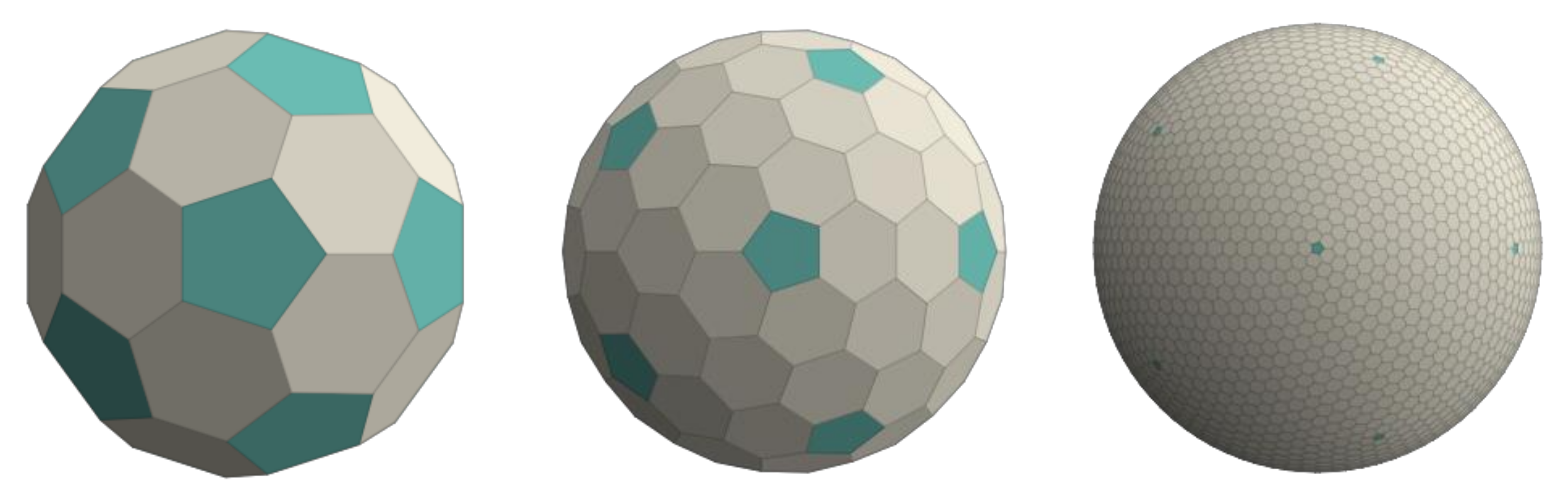
In the research, a grid of regular shapes forming Goldberg polyhedra represented the Martian areoid. This approach, proposed in 1937 by Michael Goldberg, creates a grid of hexagons and pentagons on a sphere or ellipsoid, beginning with a regular icosahedron (
Figure 1). Regardless of the number of iterations, a Goldberg polyhedron always has 12 regular pentagons and (depending on the accuracy of the projection) a number of hexagons. The research used a polyhedron composed of 4002 polygons as the approximation of the Martian areoid: 12 pentagons and 3990 hexagons. While the authors selected this number to allow fast parallel computing of hexagonal cellular automata, it can be parameterized and augmented freely. Increasing the number of polygons increases the detail of the model. However, it also reduces the computational efficiency of the cellular automaton that performs the complex operations within the iterative process consisting of hundreds of thousands of computational epochs. Using an approach based on spatial big data analysis and applying data science methodology, it is possible to model changes in the Martian atmosphere as well as to estimate the amount of energy needed for this process.
In the developed model, each polygon has its assigned spatial proximity and geometric features (distances, angles, azimuths, etc.), and the parameters are related to Mars’s topography and climatic conditions. The planet’s terrain was modeled in each of the hexagonal areal units as the average height, which is determined by MOLA (Mars Orbiter Laser Altimeter) hypsometric data analysis. In the model, the atmospheric parameters are assigned dynamically based on the simulation results from the Mars Climate Database. The model was implemented locally based on the Global Climate Model (MCD version 5.3 was downloaded, and the appropriate packages enabling data download were installed). This model can determine 84 atmospheric parameters for any hour of the Martian day or year and for any defined point with known coordinates on the surface of Mars. Due to the different times of Mars’ orbit around the Sun and the different calendars, the Martian year (lasting 687 Earth days) is divided into so-called
sols. A sol is the Martian equivalent of Earth’s solar day and amounts to 24 h 39 m 35.244 s. A year on Mars lasts, depending on the definition, 12 [
27], 16 [
28], 18 [
29], or 24 [
30] Martian months and 665, 672, 668, or 669 sols. The paper presupposes that the Martian year is 668 sols and 24 months long.
The research replaced continuous-time with discrete-time in the same way that the discretized space was divided into Goldberg polyhedra. The time interval used in the calculations was one sol: a single, model iteration was equal to one sol. This approach resulted in a three-dimensional cellular automaton in which both space and time were discretized (and parameterized, and they had several parameters assigned to individual cells and computational epochs. Some of these, for example, height above the Martian areoid level, remained constant for a given cell, while others, such as, temperature, pressure, CO2 content, wind force or direction, changed over time at intervals defined as a model’s parameters.
There were three stages in the process of modeling the changes in the atmospheric parameters of Mars using hexagonal cellular automata and transformation functions based on the convection–diffusion equation.
3.1. Hexagonal Cellular Automaton
A cellular automaton that reproduces, both locally and globally, the values for the atmospheric parameters from the Global Climate Model was a prerequisite for numerically simulating the changing of atmospheric parameters on Mars. In this approach, a cell is either a hexagonal or pentagonal areal unit. The authors used the finite-difference method to model this process, which was adapted to the interaction between the cells (
Figure 2). The cellular automaton’s transformation function used the relationships defined as the Laplace operator (Laplacian): a second-order differential operator in the form of a convection–diffusion equation [
31]
where the vector
K is the gas transport coefficient.
In this equation, the second-order partial derivatives define the differential model. It is possible to implement this model numerically using the Euler and the finite-difference methods. The
Handbook of Atmospheric Diffusion [
31] contains appropriate formulas defined for a square grid. This article uses hexagonal (and pentagonal) areal units for which the formulas are given in the following forms [
32].
Presupposing Equations (1)–(3), Equation (4) follows, where the
symbol represents the transformation from the differential model to the numerical model, assuming a hexagonal
or pentagonal
neighborhood.
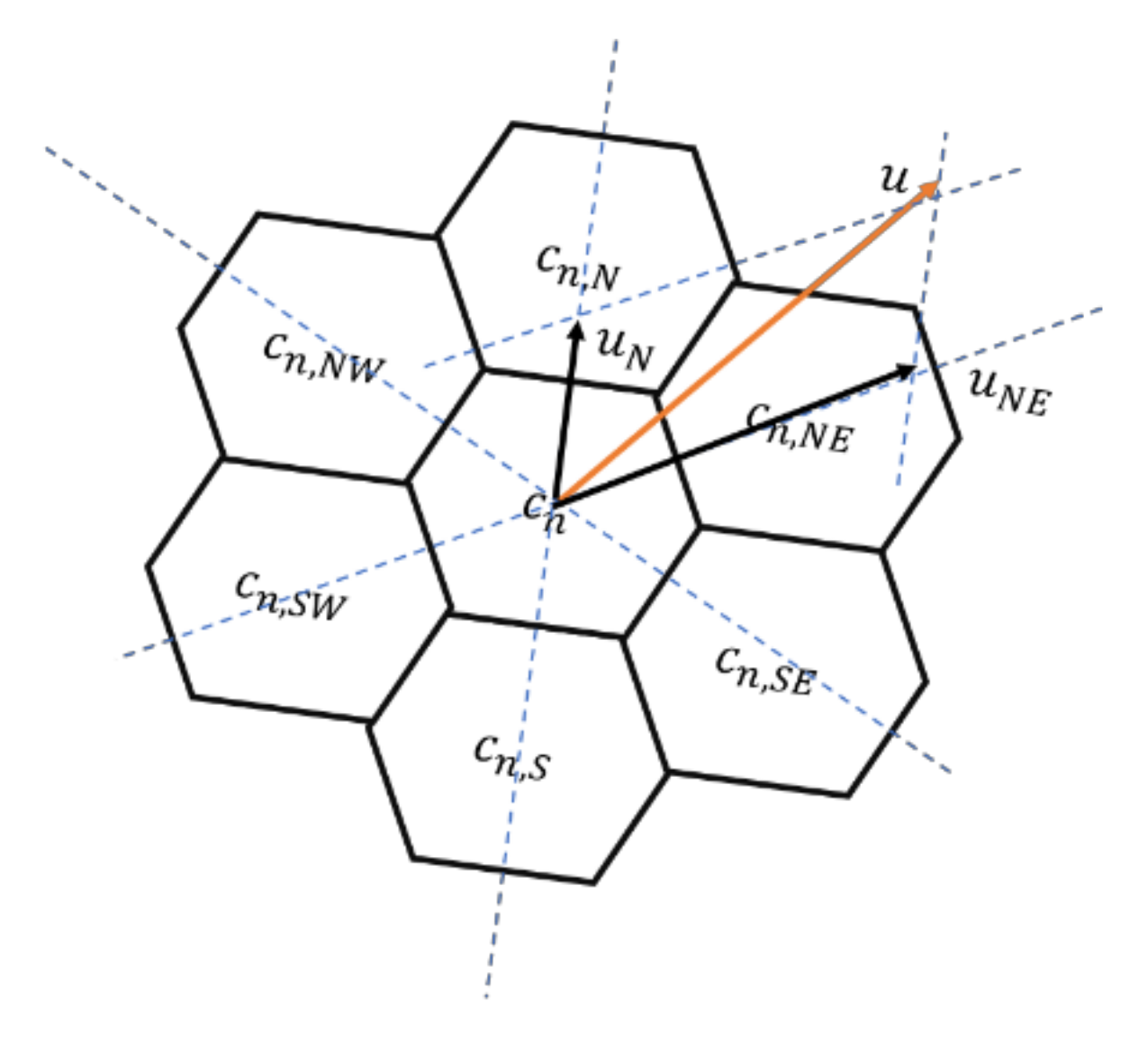
The convection–diffusion equation for the alternative that takes the wind into account (the vector
u denotes the wind vector for a given cell) (see
Figure 3) is as follows [
31]:
The following set of formulas expresses the convection–diffusion shown in Equation (5) after applying the finite-difference method for the hexagonal areal units of a cellular automaton:
For a pentagon, the transformation function takes the following form:
The eddy diffusion value,
K, was estimated for each of the considered gases (NH
3, CO
2, CFC, CH
4). When calculating the eddy diffusion for individual gases, Cussler’s estimation [
33] was used, which is based on the Chapman–Enskog theory. The assumption was that the gases diffuse in an environment composed of CO
2; averaged values for temperature
T, and pressure
P, were adopted for the entirety of Mars. Because the temperature and pressure values changed during the simulation, these values were calculated daily for the entire planet.
where
T is temperature,
A is an empirical coefficient equal to 0.001859
,
P is pressure,
is the collision coefficient of a given gas and
is the collision coefficient for CO
2, and
is the molar mass of a given gas and
is the molar mass of CO
2. The calculation has an accuracy of 8%, but this accuracy is sufficient for the model.
The following data served as the input data for the simulation: the CO
2 content for each cell (from the MCD) for the northward equinox day (vernal equinox in the northern hemisphere), the height for each cell (from the MCD and MOLA), and the wind velocity vector for each cell (from the MCD). The research enabled the analysis of compelling correlations (
Figure 4).
3.2. Including Elevation Data in the Model
The model described above implicitly assumes an interaction among flat cells of a certain shape (regular pentagons or hexagons). The area of a single cell is approximately 36,000 km
2. Due to the significant height differences on Mars (ranging from −1730 to +4920 m between individual cells, while the global variation in height difference is over 17,000 m), a simplified model using the finite element method, after one Martian year (668 sols), generates the following results: the predicted error for CO
2 pressure for each cell relative to the data was MPE = −2.01% (Mean Percentage Error), PE variance = 5.18% (Percentage Error variance), min PE = −150.34%, and max PE = 46.65% (see
Figure 5).
The research revealed that determining the CO2 content and the density of the Martian atmosphere with sufficient accuracy necessitated taking into consideration the height differences.
Because of Mars’ diverse terrain, the authors developed a linear regression model and determined its parameters in order to adapt the original approach. The model considers the height differences between a given cell and its neighbors within each hexagonal unit. This model is based on an analysis of 668 subsequent sols (a full Martian year) and the differences in values predicted by the “flat” finite element model and the Martian Global Climate Model. The obtained results indicated that it is possible to characterize the regression model correctly using a linear function:
where
y is the dependent variable: the difference between the CO
2 pressure (kg m
−2) calculated using the FDM model and the actual value in the following calculation step; and
x is the independent variable: the mean height difference (m) between a given cell and its neighbors.
The linear regression function’s linear coefficient was a = 0.00987, which means that a 100 m difference in height between one cell and another gives about 1 kg m−2 (0.987) of additional CO2 pressure.
The intercept (b) in the linear regression function is variable in time (depending on the Mars season).
The graph in
Figure 6 shows the change in the value of the linear regression function intercept across time.
After a simulation lasting 668 sols, the finite-difference model was corrected using the value from the linear regression function, which enables obtaining an accuracy level for atmospheric simulations of MPE = 0.12%, PE variance = 0.06%, min PE = −24.22%, and max PE = 60.13 %.
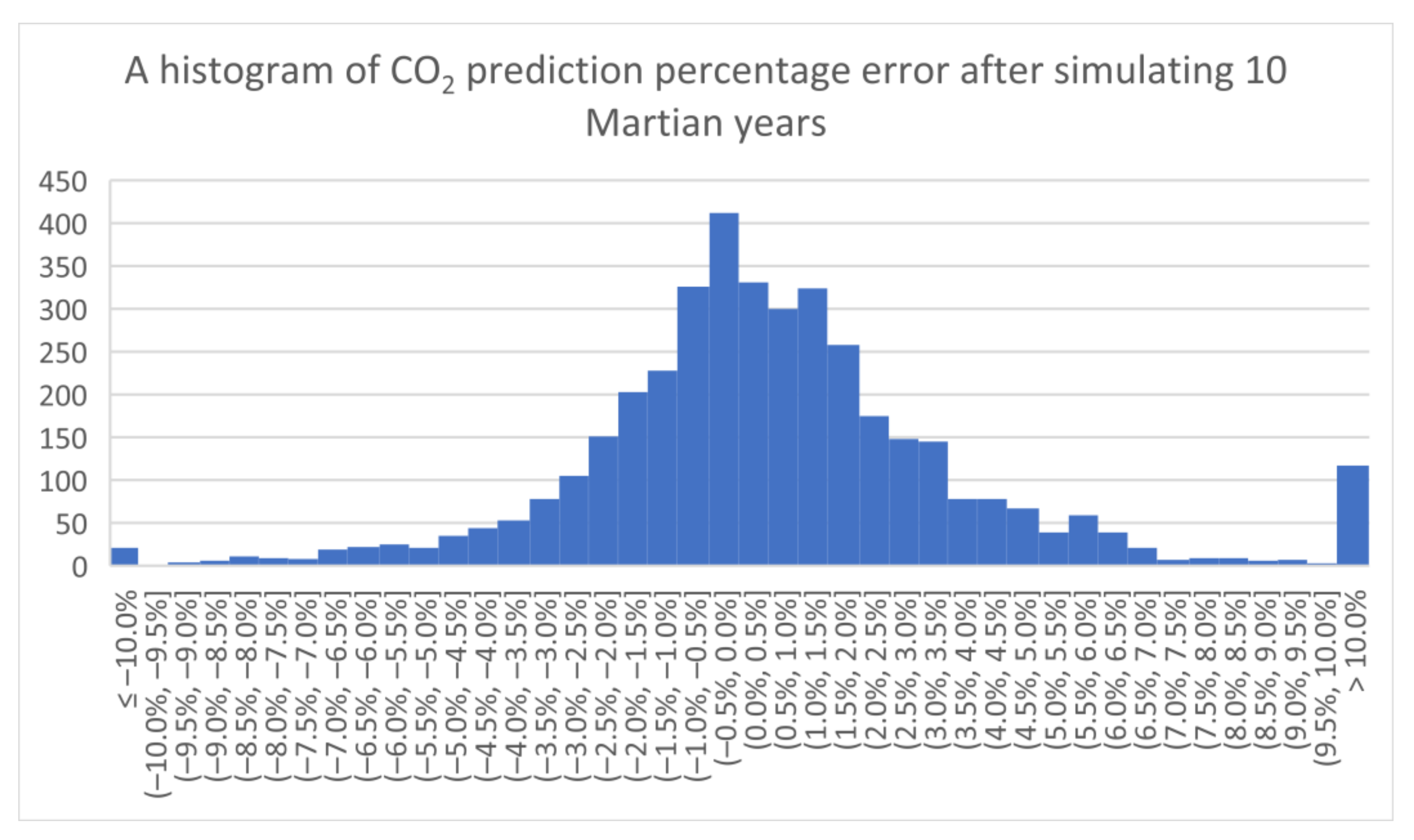
The prediction accuracy for the model remains satisfactory after the long simulation time. After 10 Martian years of simulation (13,660 iterations), the results were as follows: MPE = 0.75%, PE variance = 0.19%, min PE = −31.74%, max PE = 63.15%. The obtained results were stable and allowed for the appropriate modeling of other greenhouse gas diffusions in the Martian atmosphere: CH
4, NH
3, and CFC (see
Figure 7).
3.3. Taking into Account the Greenhouse Effect
The final stage in developing a simulation model using hexagonal cellular automata was to introduce the greenhouse effect into the model. This analysis, carried out for several alternatives, considered two terraformation scenarios for Mars:
An extension of this model is to regard each cell individually and to calculate the temperature of each cell separately. Data on Mars’s albedo for each cell were used [
20] for this purpose, and the MCD was the data source for the distance from the Sun for each sol.
This approach involved calculating the temperature rise on Mars using the Stefan–Boltzmann model, assuming a simplified heat balance of the planet using the averaged albedo of Mars and the absorption of temperature by greenhouse gasses (also potentially) in the atmosphere (CO
2, H
2O, NH
3, CH
4, CFC) (see Equation (12)).
where
is the temperature at the surface of the Sun,
is the radius of the Sun,
D is the Mars–Sun distance (changes depending on the day of the year),
is the albedo for each cell of the planet h, and
is the equivalent gray opacity of the greenhouse gasses (see Equation (13)).
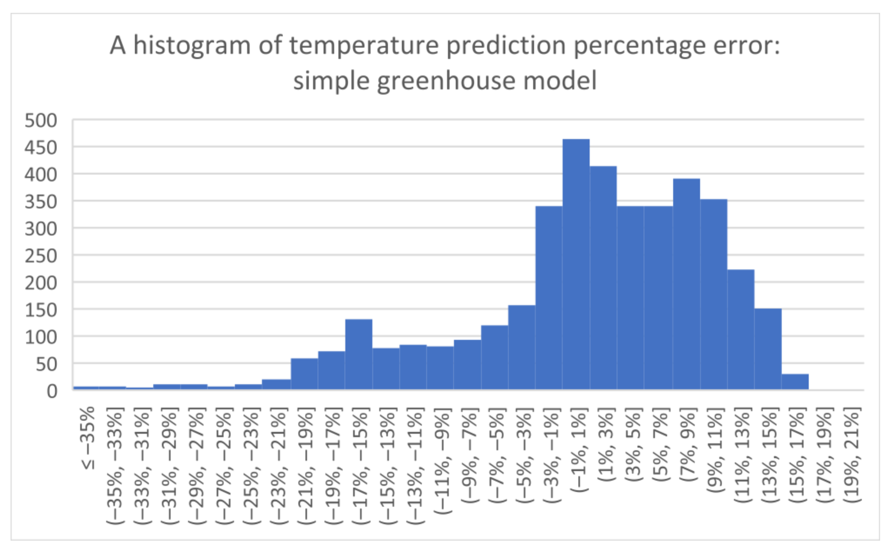
The obtained results were as follows: MPE = 0.94%, PE variance = 0.84%, min PE = −42.63%, max PE = 19.38% (see
Figure 8).
The obtained results demonstrated that the model needed further improvement. The authors searched for significant error correlations in relation to the MCD parameters. Finally, the authors used two linear regression functions in relation to the product of the heat capacity of the atmosphere (from the MCD), the temperature of the atmosphere, and the thermal flux to space (from the MCD).
This modification consisted of determining the greenhouse effect not on a global scale for the entire planet but independently for each hexagonal areal unit.
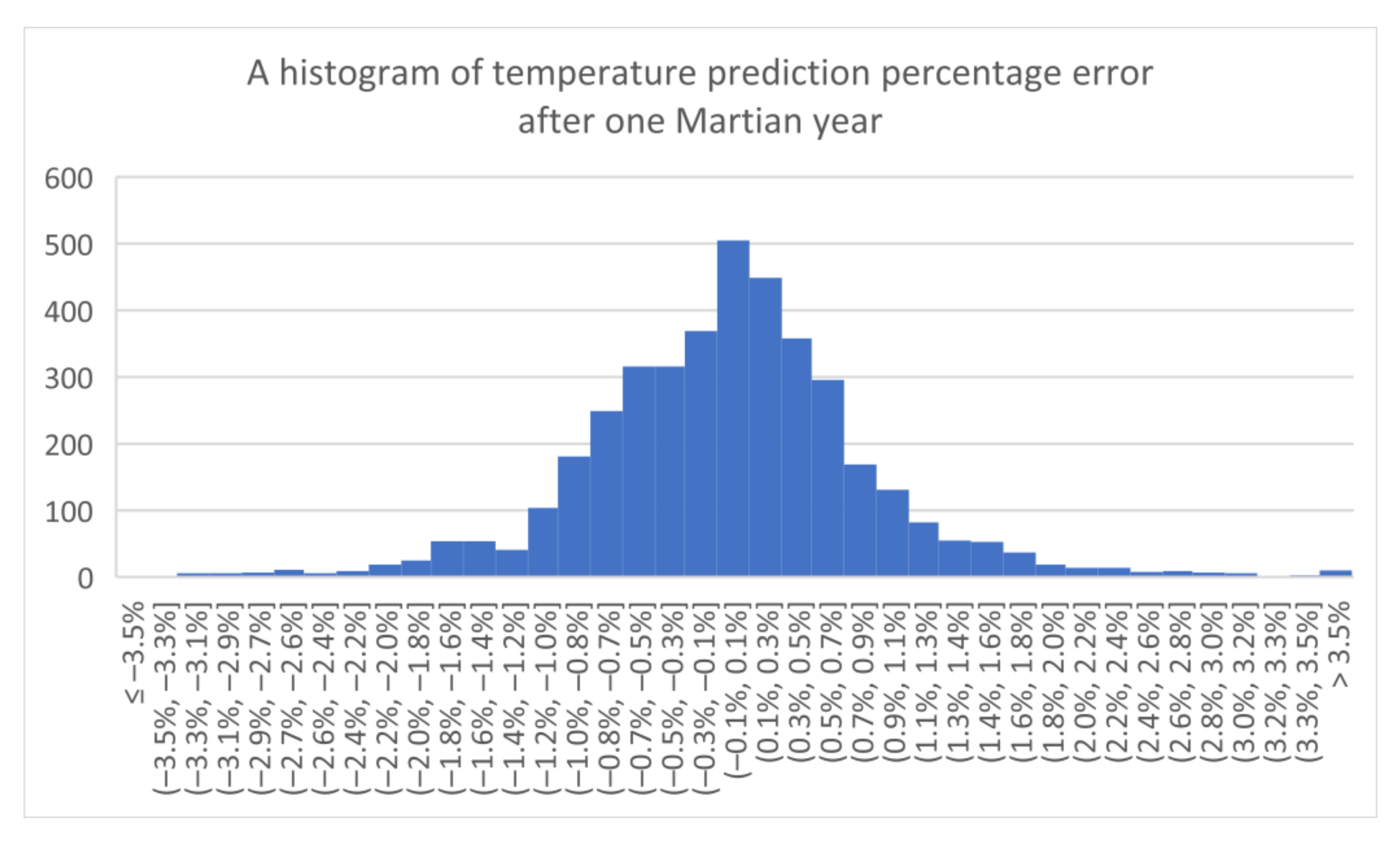
The input data consisted of the temperature of each cell on Mars on the day of the northward equinox (vernal equinox in the northern hemisphere), the albedo, the atmosphere’s heat capacity, the greenhouse gas content, and the thermal flux to space for each cell. One simulated Martian year (668 sols) generated the following temperature predictions for the Mars surface: MPE = −0.34%, PE variance = 0.04%, PE min = −7.6%, PE max = 9.57% (see
Figure 9).
4. Experiments and Analysis
4.1. Data Description and Experiment Setup
The research used atmospheric data from the MCD model and spatial and elevation data from the MOLA model. Modeling the planet’s surface required 4002 Goldberg polyhedra, 12 of which—distributed evenly over the surface of Mars—were pentagons, the rest are hexagons (
Figure 2). For each of the 4002 points constituting the centroids of the Goldberg polyhedra, 84 MCD atmospheric parameters were determined for each of 668 sols (Martian days). The main reason for selecting the data (MCD and MOLA) for the computational experiment was its reliability as well as its availability and completeness.
The modeling tool for changing the atmospheric conditions on Mars used the GAMA development environment to process the parameters mentioned above during the numerical simulation process. The process for modeling atmospheric changes also used the parameters that characterized individual greenhouse gasses used in numerical experiments (
Table 1).
Since they affect the obtained results, determining the gray opacity and the eddy diffusion parameters for individual gasses was crucial in this research. The former characterizes each gas’s greenhouse potential directly, while the latter describes the speed of the diffusion processes, which is essential in relation to the force and direction of the wind, i.e., the atmospheric parameters from the MCD model. For example, the analysis in
Table 2 indicates that for a given wind force and assuming the eddy diffusion influence for CO2 is unitary, it is one and a half times greater for ammonia and one-third smaller for Freon (chlorofluorocarbons).
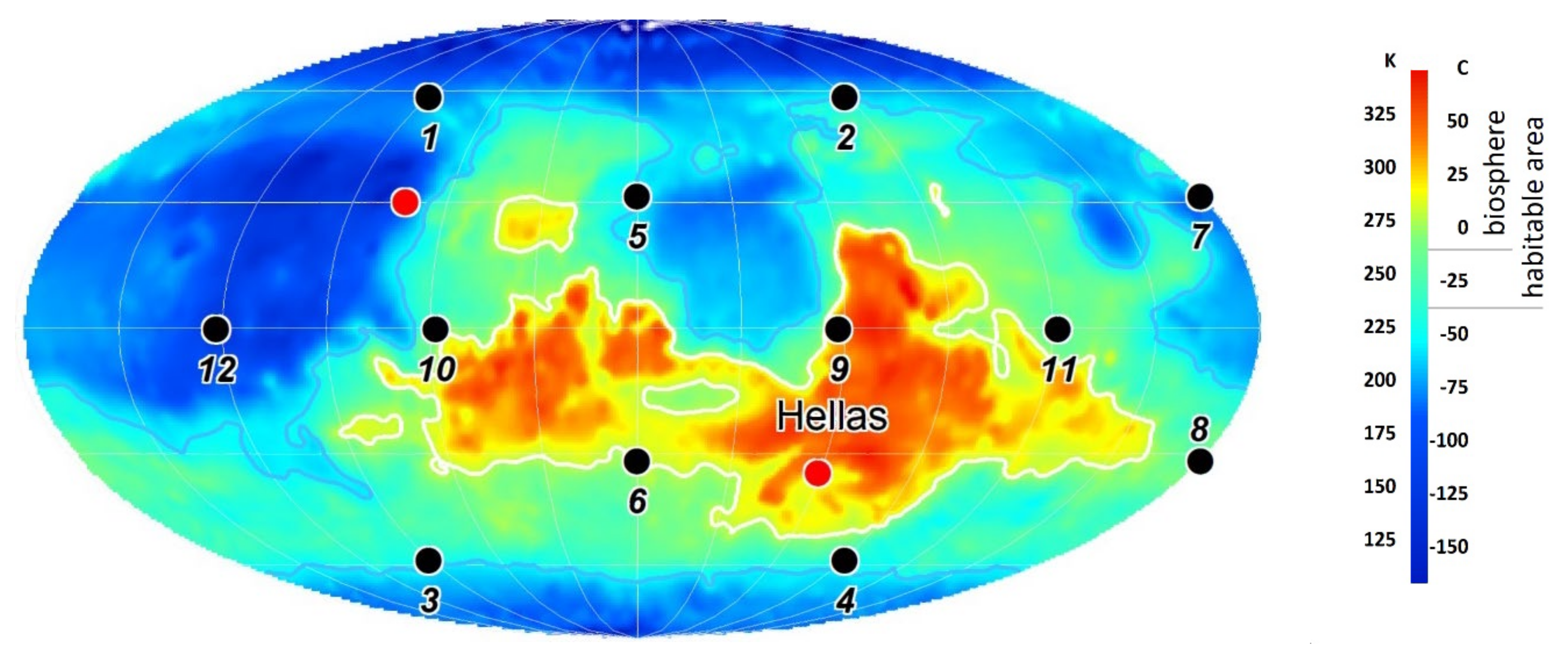
The system for modeling the process of modifying the Martian atmosphere developed by the article’s authors is fully able to be parameterized and allows for multi-variant numerical simulations. While conducting this research, the authors considered many spatial locations for the virtual greenhouse gas “factories”, asteroid “impact” sites, and simulation durations varied across time. The map (
Figure 10) shows two red points (Hellas and Tempe), which will be used further in this article to present the simulation results.
Table 2 specifies these locations’ parameters based on the MCD model for the first sol of a given Martian year. One of these points was in the southern hemisphere, on the Hellas plain inside a nearly nine-kilometer-deep impact basin, which had a pressure of 840 Pa; the other was in the northern hemisphere in the Tempe region. The choice of this region stemmed from its relatively favorable weather conditions. The design studio ABIBOO designed NÜWA city (
https://abiboo.com/projects/nuwa/, accessed on 1 July 2022) for future colonists for a location near a cliff in the Tempe region. Moreover, the analysis also included the location of virtual “greenhouse gas factories” located at 12 points that were evenly distributed across the planet’s surface.
The numerical analyzes were iterative, assuming both spatial and temporal discretization. At each calculation step (two steps corresponding to one sol), the atmospheric parameters for all 4002 areal units were modified based on the cellular automaton’s transformation function described in
Section 4. The simulations were conducted for 100 Martian years (approx. 188 Earth years); thus, it was necessary to carry out 133,600 iterations for each of the analyzed alternatives.
The results of the numerical simulations corresponded to the hexagonal (and pentagonal) areal units, which were then interpolated, enabling the visualization of the results in the form of continuous surfaces, with individual parameters varying in intensity, for example, temperature. The conducted analyses facilitated the modeling of changes in temperature, pressure, and the content of separate greenhouse gases in the atmosphere and the designation of areas with specific traits. The resulting maps and graphs showed habitable areas with temperatures above −25 °C (248.15 K) and a biosphere above 0 °C (273.15 K).
4.2. Results
The conducted research analyzed the influence of factors such as the type of greenhouse gas used, the duration of the terraformation process, the location of the gas release sites on the planet’s surface, and the intensity of this process on changes to Mars’s temperature. In the modeling, the last factor concerned the choice of either a “factory” for greenhouse gasses, which would gradually be released into the atmosphere; or an “asteroid impact,” meaning the single release of a large amount of gas at a selected point. The description of results discusses the modeling results in relation to the spatial location of the greenhouse gas release sites in the simulation process. All simulations were carried out over 100 Martian years; however, the terraformation effects are presented for the first sol of the Martian year to compare results.
4.3. Hellas
This choice of location presupposed the release of the greenhouse gas at latitude −34,595, longitude 58,982, and a height, in relation to the areoid, of −6894.5. This gas would be released by either a single impact of a cometary nucleus with a high ammonia content (100 gigatons) or ammonia production in a greenhouse gas “factory” located at this point. If this “factory” produced 1.5 megatons of ammonia per sol, this creates a similar volume of greenhouse gas (1.5 MT × 668 × 95 = 95.2 GT) to the cometary nucleus. In this simulation alternative, the gas would be produced for 95 years; the remaining five years (3340 iterations) are for the gas to stabilize. The spatial distribution of all greenhouse gases on the planet results from eddy diffusion and wind.
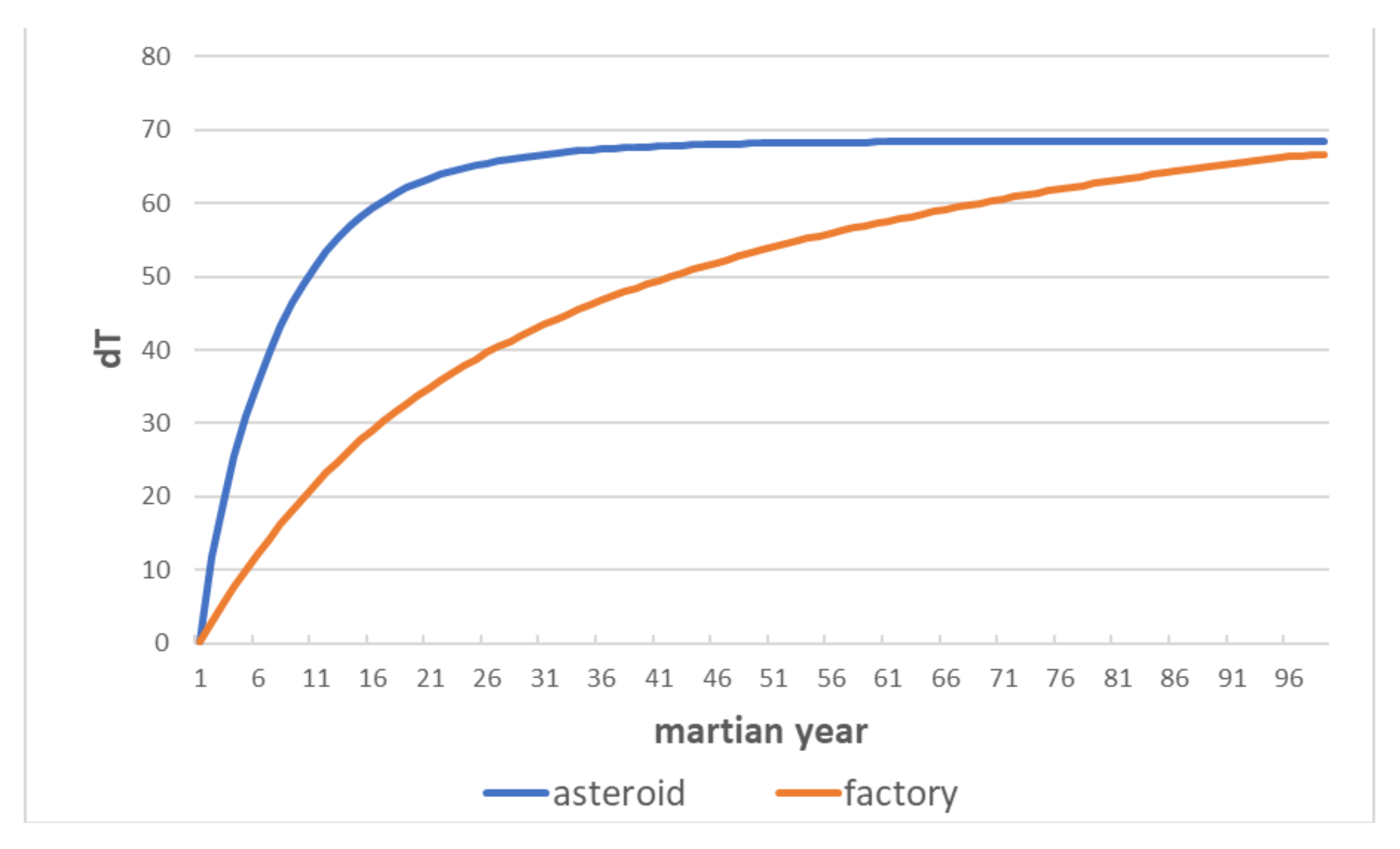
The obtained results (
Figure 11 and
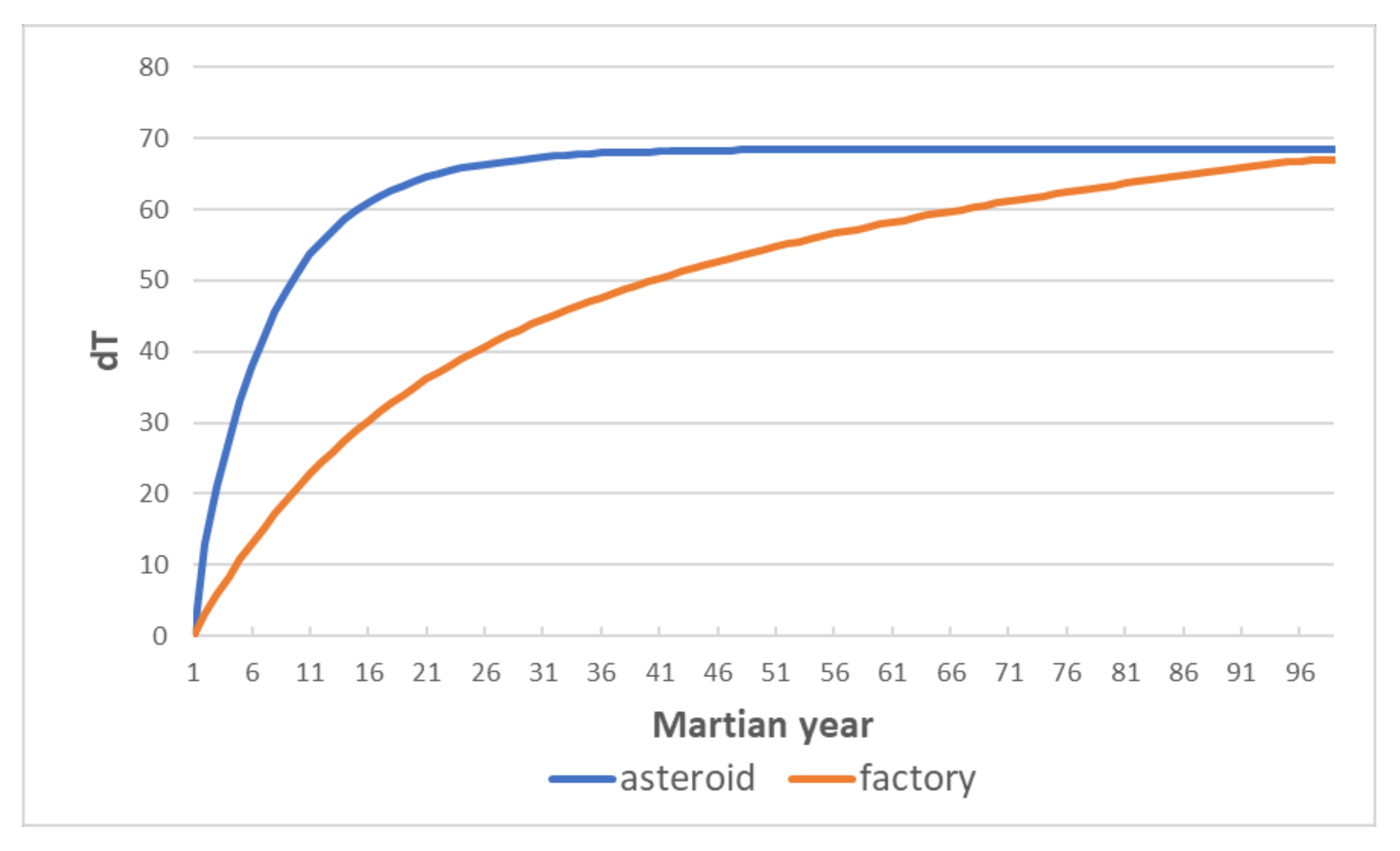
Figure 12) indicate that when using numerical parameters appropriate for ammonia in the simulation process, the average temperature increase on Mars exceeded 60 K, regardless of whether the NH
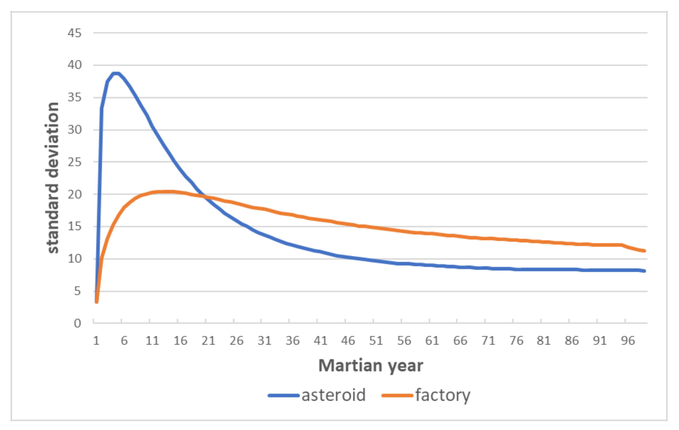
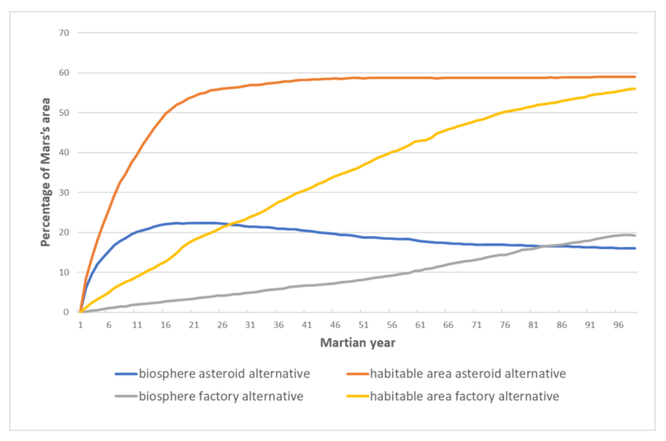
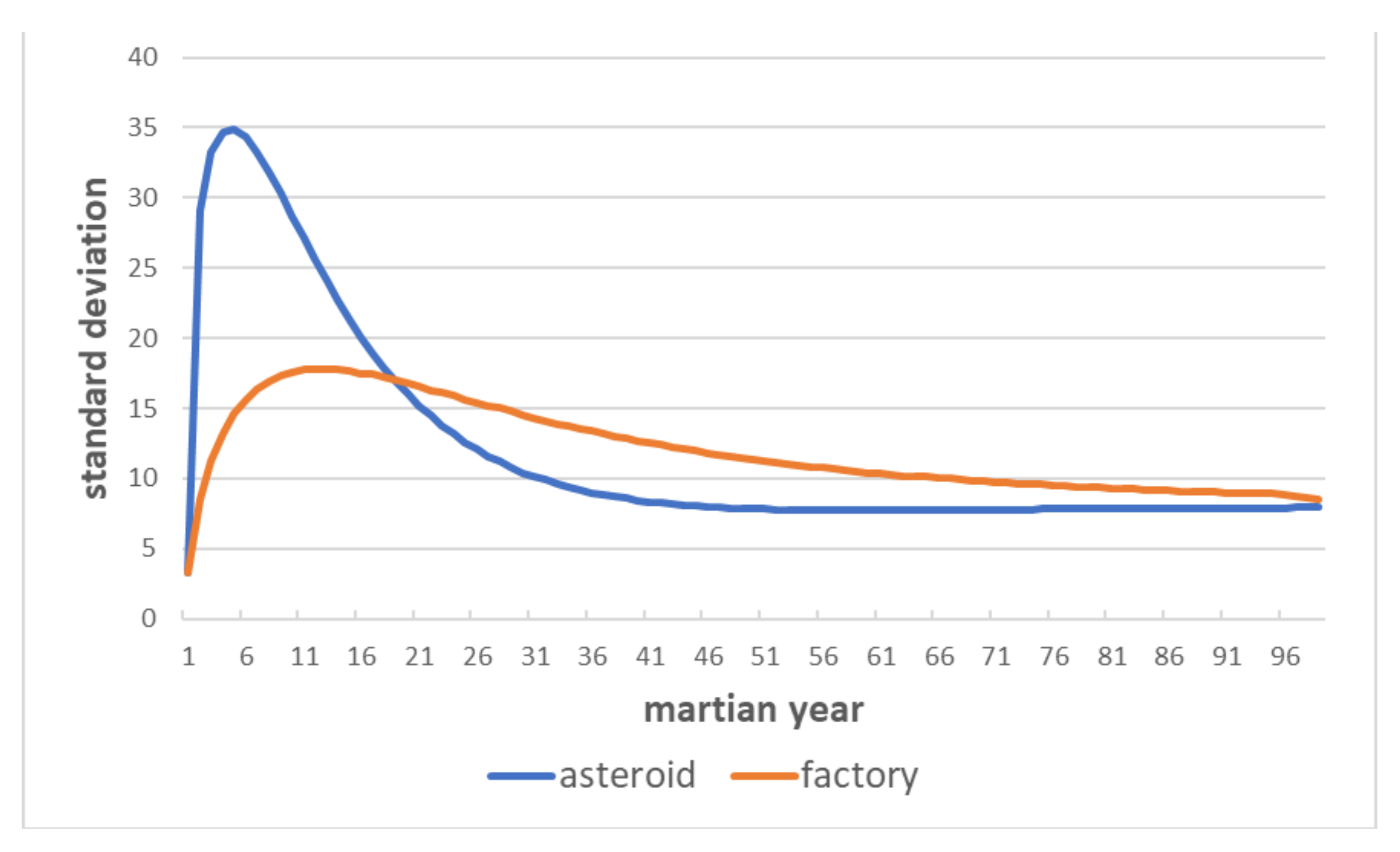
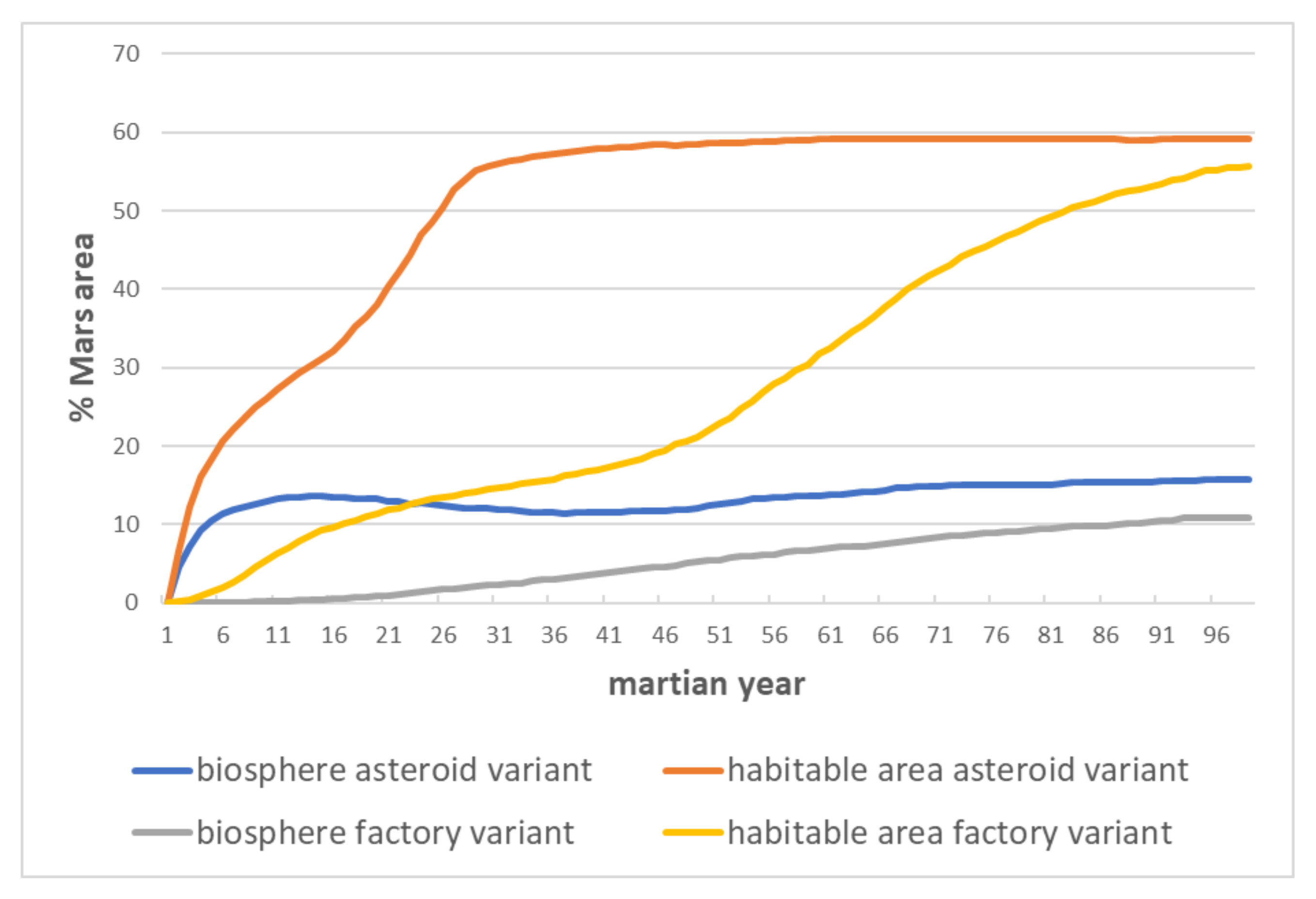
3 release was one-off or successive. However, the temperature rise graph analysis proved interesting: while the temperature rises more slowly in the “factory” alternative than in that of the “asteroid impact,” the increase was monotonic in both cases. Nevertheless, the change in time of the variance and its standard deviation (calculated relative to the mean value of the temperature rise on Mars in a given year) indicates that in the case of a rapid gas release, there are very high local interferences and significant spatial differences in the temperature distribution (in the initial phase of this process, the standard deviation was four times higher than in the final phase). The variance is much smaller in the gradual gas release case, although it still remains observable. The outcomes of these processes are visible in the difference in the size of the areas that have temperatures exceeding 0 degrees Celsius. In the case of the “asteroid,” the change diagram (
Figure 13 and
Figure 14) shows a lack of monotonicity, which is the system’s dynamic response to the impulse caused by the rapid release of NH
3. In line with control theory, the change of temperature enables parameterizing the system in terms of the growth of the biologically active zone on Mars. In the alternative for a gradual increase in greenhouse gas content, this effect is not observable; the zone above 0 C and the zone above −25 C increase their size almost linearly.
It is interesting to compare the spatial distribution of NH
3 in the Martian atmosphere after completing the 100-year simulation.
Figure 15 shows the differentiation in the case of gradual gas release: at an average of 65 kg/m
2, it is evident that the extreme values (39–120) are spatially correlated with the ammonia “factory” location. In the case of a rapid release of 100 GT of NH
3, the 100-year simulation demonstrates that despite the ammonia’s low eddy diffusion value, the spatial distribution of this gas is almost homogeneous (
Figure 15).
4.4. Tempe
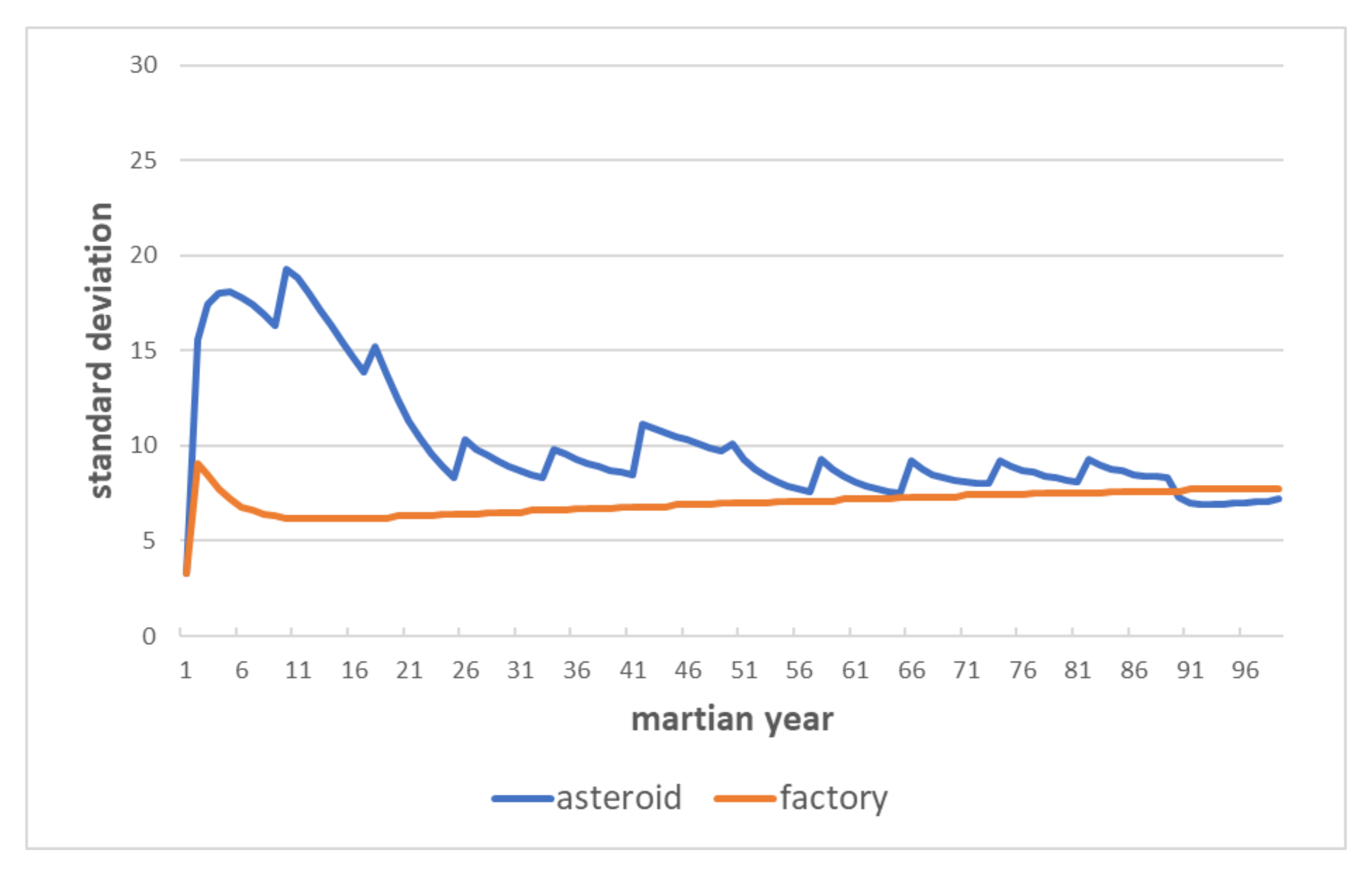
This model presupposes that the greenhouse gas is released at latitude 30.3, longitude −73.0 and a height, relative to the areoid, of −210.9. In the base version of this analysis, the gas was ammonia. As in the Hellas case, the release the greenhouse gas is either via the single impact of a cometary nucleus that has a high ammonia content (100 gigatons) or by ammonia production in a greenhouse gas “factory” located at this site. Because of the close similarity between both models, the description focuses on the differences that stem from the different topographic conditions. The Tempe region is in the northern hemisphere and is much higher than the Hellas basin, which means that the atmospheric conditions are significantly different: the temperature is more than 30 degrees lower, the pressure is almost twice as low, and the winds are almost three times stronger.
The obtained results indicate that a period of 100 Martian years (almost 190 Earth years) is sufficient to almost entirely homogenize the spatial distribution of temperature after the rapid release of 100 GT of NH
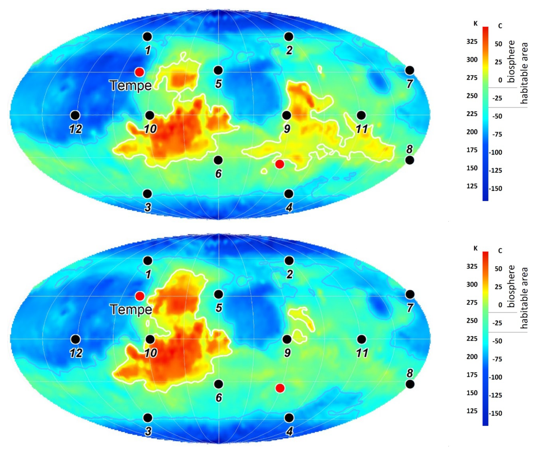
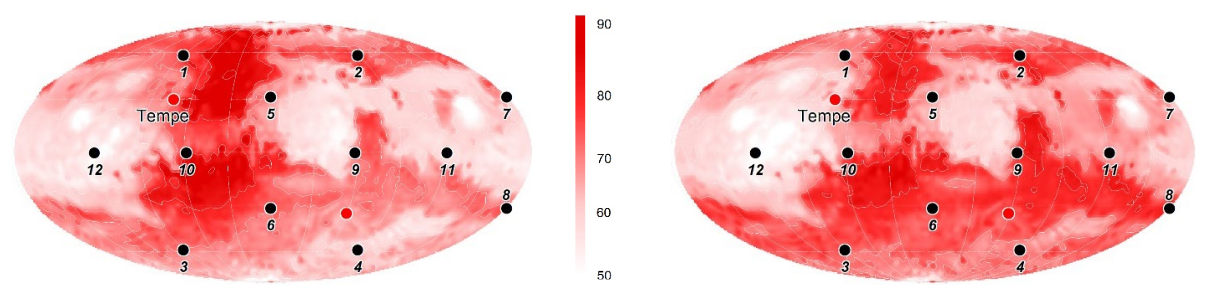
3 in both the Tempe and Hellas regions. However, the gradual gas release model is dissimilar; there is a significant difference in the spatial distribution of the temperature increase between these greenhouse gas “factories” locations. Interestingly, the temperature did not increase maximally in the vicinity of the gas production site (
Figure 16 and
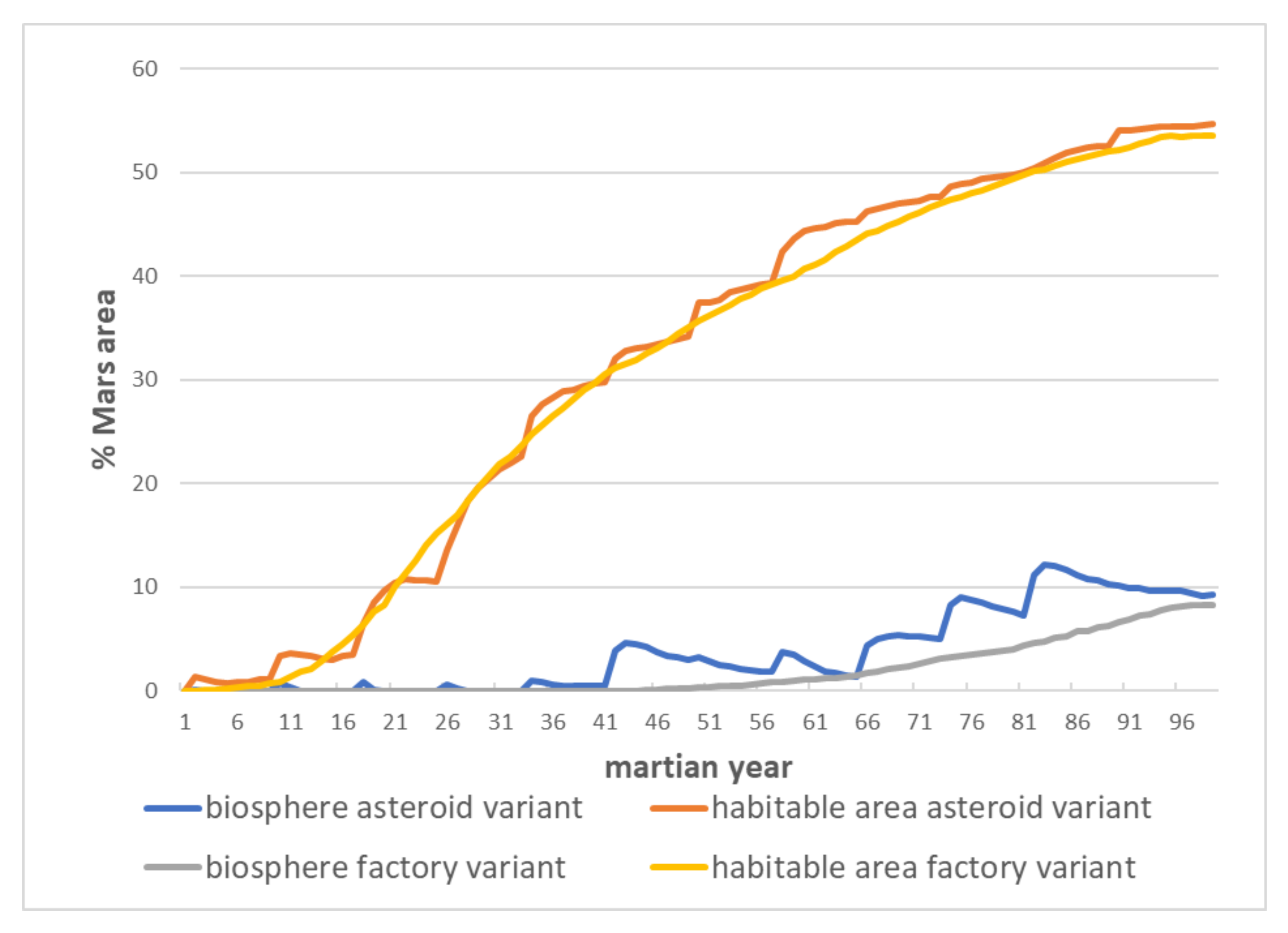
Figure 17). Instead, due to strong latitudinal winds and the Martian terrain in this region, the highest increase was achieved in the Chryse and Acidalia region, east of Tempe. What is also noteworthy is the time-variable growth rate for the zone that had average temperatures exceeding 0 °C and −25 °C. In the case of the zone that had greater than 0 °C, due to the system’s dynamic response to the rapid release of 100 GT of NH
3, the change in the size of the biologically active zone is non-monotonic, while for the zone that had over −25 °C, it was non-linear (
Figure 18,
Figure 19 and
Figure 20). For the gradual gas release alternative, the change in size for both zones was almost linear, but the absolute values of the temperature rise are lower.
4.5. Twelve Locations
In order to do an in-depth analysis of what influence the site where the greenhouse gases are released has on the outcome of terraformation, the authors developed a model in which the gas is released at 12 locations evenly distributed over the entire Martian surface. As in the Hellas and Tempe models, this model also considers the differentiation in the intensity of gas release between the “asteroid” and “factory” alternatives. To ensure the comparability of the results, in both cases, the volume of gas released at a given point was reduced by 12 times, so after 100 Martian years, there would be 100 GT of ammonia in total released into the planet’s atmosphere.
The first model presupposes that every eight years, a cometary nucleus containing 8.3 GT of NH3 hits points with successive identifiers from 1 to 12. The second model presupposes that during the initial 95 years of the simulation, each of the 12 points produces 125 kT of ammonia per sol. The results indicate an average increase in the planet’s temperature of over 60 °C, which is similar to the previously considered models but with different spatial and temporal differentiation.
The very high variation in temperature rise during the initial phase of the modeling process contributed to the highly complex development of the biologically active zone. During the initial phase (about 40 Martian years), the increase in the over 0 °C zone was almost zero, but in the following 60 years, it changed abruptly and non-monotonically. In the simulation that included creating 12 greenhouse gas “factories,” after almost half a century (in Martian years) without a change, there was an increase of a linear nature (
Figure 21 and
Figure 22).
Notably, the average temperature increase after 100 years was slightly lower (approx. 2K) in the case of the 12 smaller asteroids, which is in contrast to the one asteroid with an NH
3 volume of 100 GT. Interestingly, the spatial distribution of the temperature and the ammonia content in the atmosphere differed significantly from the single-point gas release model. This was particularly evident for the spatial distribution of ammonia—in the alternative with the 12 “factories,” the NH
3 content was visibly higher than the average at the gas release points; in the variant with the 12 “asteroids,” the influence of the time over which the gas was released into the atmosphere was visible (
Figure 23 and
Figure 24).
Figure 25 shows that the four years after the asteroid’s impact at id = point 12, and the 12 years from the impact at id = point 11 were not enough time for the wind and eddy diffusion to balance the spatial distribution of ammonia on the planet.
5. Energy Expenditure
The postulated variants leading to terraformation are massive undertakings with a high execution cost. One of the essential components of these costs is the energy expenditure leading to implementing each of the variants.
5.1. Asteroid Impact
We assume that the asteroid of mass
will be brought in from the Kuiper belt (30–50 AU—astronomical units), where the ammonia-built asteroids are located. In order to bring such an object to Mars, its orbit should be changed—by appropriate speed correction—and then, gravity assist of Mars should be used. In [
6], an analysis of the bringing of celestial body depending on its distance from the Sun was carried out. The results state × that the farther an object is from the Sun, the less velocity correction needed to be applied. For the asteroids from the Kuiper belt, the required velocity correction is between 0 and 500 m/s. Assume the needed speed change is
.
Methods of changing the celestial object’s orbit are described in the paper [
38]. In order to change the speed of an object by
, there is a need to change its kinetic energy. Such energy can be provided by, inter alia, the delivery and explosion of a nuclear bomb or by a mass ejection caused by the vaporization of the gaseous portion of the asteroid.
The nuclear energy needed for bringing one 100 GT asteroid is at least 4500 × 10
15 J, which corresponds to a nuclear reaction in which about 55 Mg of U-235 is converted into energy. Launching 1 kg of mass needs 1 MJ energy. For this case, the Falcon Heavy SpaceX rocket is needed [
https://www.spacex.com/vehicles/falcon-heavy/, accessed on 1 July 2022] to have enough payload. The rocket’s mass is 1.4 × 10
6 kg, so the energy needed to launch the payload is equal to 1.4 × 10
12 J. For launching 12 smaller bombs, the Falcon 9 SpaceX rocket is enough [
https://www.spacex.com/vehicles/falcon-9/, accessed on 1 July 2022]. The mass 550× 10
3 kg results in the energy needed to launch a single rocket into space being equal to 5.5× 10
8 J (
Table 3).
The latter method is based on a mass ejection, discussed in [
6]. Building on their calculations, heating up the ammonia on 10 (GT) asteroid to 2200 K requires 4 thermal rocket engines of power 5000 (MW) thrusting the asteroid for 10 years. The energy of a single thermal rocket working by 10 years is equal to 157.68× 10
15 (J), and it is enough to thrust a mass of 2.5 (GT). Assume a single Falcon 9 rocket per single thermal power engine gives us the results (see
Table 4). The calculations for 12 asteroids are omitted due to similar results.
5.2. Greenhouse Gasses Production
In [
14], an analysis of production halocarbons (CFC) on Mars is discussed. According to these assumptions, the production of 1 T of CFC per hour requires the power of 5 MW. Thus, 1 T of CFC per Martian year production requires 80 GJ of energy. Note, however, that the calculations do not include building and maintaining a power plant and the factories. Maintaining twelve GHG factories seems to be more energy consuming. Moreover, taking into account possible uncertainties, for example, potential energy loss in the transition through the many sub-factories, the one-factory scenario is more favorable. Note however, that from the point of view of the potential failure, production scattering across multiple sites seems to be a better approach.
The obtained approximate energy costs of the variants: changes in the asteroid course caused by a nuclear charge impact and mass ejection from the asteroid. The greenhouse gas production on Mars provides us with comparisons of these costs. In the order of 90 × 10
12 J, the smallest costs were estimated for the production of greenhouse gases (CFCs) on the surface of Mars (
Table 5). However, it should be noted that they do not consider the costs of providing appropriate infrastructure (power plants, factory elements) to Mars. The energy costs of fetching asteroids are about three orders higher.
6. Discussion
While conducting this research, the authors assumed that carbon dioxide is released from the regolith in gas form due to temperature changes. Based on the work of [
39], the authors assumed that the total mobilizable CO
2 (polar ice and near-surface carbonates) would be sufficient to increase the pressure on Mars by ≈0.020 bar. Accomplishing this process requires ≈6000 × 10
15 J energy with the asteroid impact variant and ≈100 × 10
12 J with the production of greenhouse gases on the surface of Mars.
The authors noted that applying an asteroid “impact” caused a very high local concentration of gas, and, hence, a considerable local temperature increase (bear in mind that the model does not take into account the temperature increase resulting from the “impact” of the asteroid itself). A greenhouse gas “factory” leads to a stable increase in gas concentration and temperature.
The research analyzed the influence of the greenhouse gas “factories” location, their number, the amount of gasses released into the atmosphere, and the duration of the simulation for the obtained results. For instance, the location of 12 small “factories” on Mars’s surface enables 8% of the surface with a temperature exceeding 0 °C to be acquired over the subsequent 100 years, while the location of one large “factory” in the Tempe region results in a 10% coverage of a biologically active zone, and for Hellas, as much as 18%. Thus, it is not only the volume and type of greenhouse gasses that are important but also the production and release site. The alternative utilizing an asteroid “impact” achieved similar results. The release of 100 GT of NH3 in one place results in 15% of the surface area having liquid-water reserves, while dividing this value into 12 smaller ones leads to only a 9% surface area.
Analyzing the correlation matrix for particular parameters that have been determined for different spatial locations produces exciting results. Compiling the values for absolute and relative heights, temperature, pressure, wind force and direction, and several dozen other atmospheric parameters for 4002 points on the surface of Mars means a matrix can be developed for partial correlation between individual factors. The analysis of this matrix reveals that no leading factor has a decisive influence on temperature increase at any given point. Therefore, many interdependent factors influence the climatic parameters (such as temperature) in a dynamic, non-linear, and complex manner. The developed tool facilitates the simulation of many alternative models and can provide answers to “what if?” questions.
7. Conclusions
From the perspective of the technological development of Earth’s civilization, 100 Martian years, i.e., less than 200 Earth years, is a reasonable period for the first stage of terraformation of the planet, i.e., warming of 60 K and increasing the atmosphere density. Starting the terraformation process using greenhouse gasses at the end of the first half of the twentieth century would have led to a temperature increase of about 60 K by the end of the twenty-first century, significantly streamlining the colonization of Mars. One should remember that increasing the temperature is a sine qua non for life on Mars to be able to function as it does on Earth; however, it is not enough. Nonetheless, it is the first step toward the terraforming of this planet.
The developed methodology for modeling the process of terraforming the Martian atmosphere using hexagonal cellular automata can produce multi-variant simulations of climate change on the Red Planet. The devised simulation tool is based on open-source tools and has been made available as source code (
https://github.com/piotrpowerpalka/mars_terraforming, accessed on 1 July 2022). Algorithms for modifying climate parameters use publicly available MOLA spatial elevation data, the MCD atmospheric model, eddy diffusion models, and numerical simulation methodology using cellular automata that enable spatial and temporal discretization.
The research has shown that it is possible to develop a numerical simulation system that can model the spatial and temporal variability of the atmospheric parameters on Mars. This model is fully able to be parameterized, which helps in calculating the release sites and volume of greenhouse gas, the intensity of the process, and changes to the chemical composition of the gas. The developed tool can analyze changes over time and visualize the spatial distribution of individual parameters for any calculation step.
When conducting numerical research, the authors disregarded the issue of technological possibilities and the costs of the potential implementation of individual alternatives, such as constructing a greenhouse gas “factory” on Mars, or bringing an asteroid that has a high methane content from the asteroid belt between Mars and Jupiter. The research aimed only to analyze the atmospheric effects of the potential terraformation of Mars. The conducted research has shown that the release of 100 GT of CFCs or methane into the planet’s atmosphere would raise the average temperature of Mars by several degrees within 100 Martian years (about 188 Earth years). This value (100 GT) is relatively small in relation to the mass of greenhouse gases produced on Earth [
40]. Using other greenhouse gasses, for example, ammonia, would increase the greenhouse effect by an order of magnitude. The simulations have also demonstrated the significance of the location of the greenhouse gas “factory” and the process’s intensity.
The approach of building an atmospheric model of Mars using analytical models in conjunction with big data analysis of data provided by missions is a good tool for what-if analysis, which was justified by the results obtained. We plan to extend the analytical model with a new variant of the cell energy balance, taking into account the phase changes of carbon dioxide. In addition, we are planning further analyses of planet representation using the Goldberg polyhedral with higher resolution (25,000 polygons).
It should be emphasized that for obtaining the greenhouse effect described in this article, a significant amount of energy is needed. Conducted research have shown that terraforming Mars atmosphere by bringing the asteroid and causing its impact requires the use of energy about three orders of magnitude bigger than necessary for building greenhouse gas factories on the planet surface. This second solution, however, requires taking into account costs (also energy) of bringing from Earth appropriate technical infrastructure.
Author Contributions
Conceptualization, P.P. and R.O.; methodology, P.P. and R.O.; software, P.P.; validation, A.W.; formal analysis, A.W.; investigation, P.P. and R.O.; resources, R.O.; data curation, P.P.; writing—original draft preparation, P.P. and R.O.; writing—review and editing, A.W..; visualization, R.O.; supervision, R.O; project administration, A.W.; funding acquisition, R.O. All authors have read and agreed to the published version of the manuscript.
Funding
The project was funded by the POB Research Centre Cybersecurity and Data Science of Warsaw University of Technology within the Excellence Initiative Program—Research University (ID-UB).
Informed Consent Statement
Not applicable.
Data Availability Statement
Conflicts of Interest
The authors declare no conflict of interest.
References
- Mars 2020 Mission Contributions to NASA’s Mars Exploration Program Science Goal. 2007; Volume 3, pp. 154–196. Available online: https://mars.nasa.gov/mars2020/mission/science/goals/ (accessed on 1 July 2022).
- Sagan, C. Planetary Engineering of Mars. Icarus 1973, 20, 513–514. [Google Scholar] [CrossRef]
- Averner, M.M.; MacElroy, R.D. On the Habitability of Mars: An Approach to Planetary Ecosynthesis; NASA SP-414; National Aeronautics and Space Administration: Washington, DC, USA, 1976.
- Lovelock, J.E.; Allaby, M. The Greening of Mars; Warner Brothers Inc.: New York, NY, USA, 1984. [Google Scholar]
- McKay, C.P.; Toon, O.B.; Kasting, J.F. Making Mars habitable. Nature 1991, 352, 489–496. [Google Scholar] [CrossRef] [PubMed]
- Zubrin, R.M.; McKay, C.P. Technological requirements for terraforming Mars. J. Br. Interplanet. Soc. 1997, 50, 83–92. [Google Scholar]
- Zhang, T.; Sun, S. Thermodynamics-Informed Neural Network (TINN) for Phase Equilibrium Calculations Considering Capillary Pressure. Energies 2021, 14, 7724. [Google Scholar] [CrossRef]
- Michel, P.; Kueppers, M.; Sierks, H.; Carnelli, I.; Cheng, A.F.; Mellab, K.; Granvik, M.; Kestilä, A.; Kohout, T.; Muinonen, K.; et al. European component of the AIDA mission to a binary asteroid: Characterization and interpretation of the impact of the DART mission. Adv. Space Res. 2018, 62, 2261–2272. [Google Scholar] [CrossRef] [Green Version]
- Zhang, T.; Yiteng, L.; Chen, Y.; Feng, X.; Zhu, X.; Chen, Z.; Yao, J.; Zheng, Y.; Cai, J.; Song, H.; et al. Review on space energy. Appl. Energy 2021, 292, 116896. [Google Scholar] [CrossRef]
- Hansen, J.; Nazarenko, L.; Ruedy, R.; Sato, M.; Willis, J.; Del Genio, A.; Koch, D.; Lacis, A.; Lo, K.; Menon, S.; et al. Earth’s energy imbalance: Confirmation and implications. Science 2005, 308, 1431–1435. [Google Scholar] [CrossRef] [Green Version]
- Kushnir, Y. Solar Radiation and the Earth’s Energy Balance; Published on The Climate System, Complete Online Course Material from the Department of Earth and Environmental Sciences at Columbia University; Department of Earth and Environmental Sciences at Columbia University: New York, NY, USA, 2000; p. 2008. [Google Scholar]
- Travis, B.; Rosenberg, N.; Cuzzi, J. Geothermal heating, convective flow and ice thickness on Mars. In Proceedings of the 32nd Annual Lunar and Planetary Science Conference, Houston, TX, USA, 12–16 March 2001; p. 1390. [Google Scholar]
- Delgado-Bonal, A.; Martín-Torres, F.J.; Vázquez-Martín, S.; Zorzano, M.-P. Solar and wind exergy potentials for Mars. Energy 2016, 102, 550–558. [Google Scholar] [CrossRef]
- Sholes, S.F.; Krissansen-Totton, J.; Catling, D.C. A Maximum Subsurface Biomass on Mars from Untapped Free Energy: CO and H2 as Potential Antibiosignatures. Astrobiology 2019, 19, 655–668. [Google Scholar] [CrossRef] [PubMed] [Green Version]
- Miley, G.; Yang, X.; Rice, E. Distributed Power Sources for Mars. In Mars: Prospective Energy and Material Resources; Badescu, V., Ed.; Springer: Berlin/Heidelberg, Germany, 2009; pp. 213–239. [Google Scholar]
- Palaia, J.E., IV; Homnick, M.S.; Crossman, F.; Stimpson, A.; Truett, J. Economics of Energy on Mars. In Mars: Prospective Energy and Material Resources; Badescu, V., Ed.; Springer: Berlin/Heidelberg, Germany, 2009; pp. 369–400. [Google Scholar]
- Fogg, M.J. Terraforming Mars: A review of current research. Adv. Space Rer. 1998, 22, 415–420. [Google Scholar] [CrossRef]
- Burns, J.A.; Harwit, M. Towards a more habitable Mars—or—the coming Martian spring. Icarus 1973, 19, 126–130. [Google Scholar] [CrossRef]
- Badescu, V.; Isvoranu, D.; Cathcart, R.B. Ecopoiesis and Liquid Water Transportation on Mars. In Mars: Prospective Energy and Material Resources; Badescu, V., Ed.; Springer: Berlin/Heidelberg, Germany, 2009; pp. 661–682. [Google Scholar]
- Lewis, S.R.; Collins, M.; Read, P.L.; Forget, F.; Hourdin, F.; Fournier, R.R.; Hourdin, C.; Talagrand, O.; Huot, J.-P. A climate database of Mars. J. Geophys. Res. Planets 1999, 104, 24177–24194. [Google Scholar] [CrossRef]
- Millour, E.; Forget, F.; Spiga, A.; Navarro, T.; Madeleine, J.-B.; Montabone, L.; Pottier, A.; Lefevre, F.; Montmessin, F.; Chaufray, J.-Y.; et al. The Mars Climate Database (MCD version 5.2). In Proceedings of the European Planetary Science Congress 2015, EPSC2015-438, Nantes, France, 27 September–2 October 2005; Volume 10. [Google Scholar]
- Millour, E.; Forget, F.; Spiga, A.; Vals, M.; Zakharov, V.; Navarro, T.; Montabone, L.; Lefevre, F.; Montmessin, F.; Chaufray, J.-Y.; et al. The Mars Climate Database (MCD version 5.3), Geophysical Research Abstracts. In Proceedings of the EGU General Assembly 2017, EGU2017-12247, Vienna, Austria, 23–28 April 2017; Volume 19. [Google Scholar]
- Marinova, M.M.; McKay, C.P.; Hashimoto, H. Radiative-convective model of warming Mars with artificial greenhouse gasses. J. Geophys. Res. 2005, 110, E03002. [Google Scholar] [CrossRef] [Green Version]
- Christensen, P.R.; Bandfield, J.L.; Hamilton, V.E.; Ruff, S.W.; Kieffer, H.H.; Titus, T.N.; Mali, M.C.; Morris, R.V.; Lane, M.D.; Clark, R.L.; et al. The Mars Global Surveyor Thermal Emission Spectrometer experiment: Investigation description and surface science results. J. Geophys. Res. 2001, 106, 23823–23871. [Google Scholar] [CrossRef]
- Rodrigo, R.; Garcia-Alvarez, E.; Lopez-Gonzales, M.J.; Lopez-Valverde, M.A. Estimates of eddy diffusion coefficient in the Mars’ atmosphere. Atmosfera 1990, 3, 31–43. [Google Scholar]
- Trainer, M.G.; Wong, M.H.; McConnochie, T.H.; Franz, H.B.; Atreya, S.K.; Conrad, P.G.; Lefèvre, F.; Mahaffy, P.R.; Malespin, C.A.; Manning, H.L.; et al. Seasonal Variations in Atmospheric Composition as Measured in Gale Crater, Mars. J. Geophys. Res. Planets 2019, 124, 3000–3024. [Google Scholar] [CrossRef]
- Pickering, W.H. Report on Mars, No. 17. Pop. Astron. 1916, 24, 639. [Google Scholar]
- Aitken, R.G. Time Measures on Mars. Astron. Soc. Pac. Leafl. 1936, 2, 177. [Google Scholar]
- Moore, P. Guide to Mars; Lutterworth Press: Cambridge, UK, 1997; ISBN 0718823168. [Google Scholar]
- Gangale, T. Martian Standard Time. J. Br. Interplanet. Soc. 1986, 39, 282–288. [Google Scholar]
- Hanna, S.R.; Briggs, G.A.; Hosker, R.P., Jr. Handbook on Atmospheric Diffusion (No. DOE/TIC-11223); National Oceanic and Atmospheric Administration: Oak Ridge, TN, USA; Atmospheric Turbulence and Diffusion Lab: Oak Ridge, TN, USA, 1982. [CrossRef] [Green Version]
- Fabero, J.; Bautista, A.; Casasús, L. An Explicit Finite Differences Scheme over Hexagonal Tessellation. Appl. Math. Lett. 2001, 14, 593–598. [Google Scholar] [CrossRef] [Green Version]
- Cussler, E.L. Diffusion: Mass Transfer in Fluid Systems, 2nd ed.; Cambridge University Press: New York, NY, USA, 1997; pp. 634–639. ISBN 0-521-45078-0.2. [Google Scholar]
- McKay, C.P.; Davis, W.L. Duration of liquid water habitats on early Mars. Icarus 1991, 90, 214–221. [Google Scholar] [CrossRef]
- Buhler, P.B.; Piqueux, S. Obliquity-driven CO2 exchange between Mars’ atmosphere, regolith, and polar cap. J. Geophys. Res. Planets 2021, 126, e2020JE006759. [Google Scholar] [CrossRef]
- Levenson, B.P. Habitable zones with an earth climate history model. Planet. Space Sci. 2021, 206, 105318. [Google Scholar] [CrossRef]
- Fogg, M.J. A Synergic Approach to Terraforming Mars. Br. Interplanet. Soc. J. 1992, 45, 315–329. [Google Scholar]
- Markopoulos, N. How much thrust, energy, or propellant does it take to guide a natural celestial body? J. Astronaut. Sci. 2000, 48, 25–43. [Google Scholar] [CrossRef]
- Jakosky, B.M.; Edwards, C.S. Inventory of CO2 available for terraforming Mars. Nat. Astron. 2018, 2, 634–639. [Google Scholar] [CrossRef]
- Ritchie, H.; Roser, M. CO2 and Greenhouse Gas Emissions. Published Online at OurWorldInData.org. 2020. Available online: https://ourworldindata.org/co2-and-other-greenhouse-gas-emissions (accessed on 1 July 2022).
Figure 1.
Three different Goldberg polyhedra.
Figure 1.
Three different Goldberg polyhedra.
Figure 2.
Fragment of a Goldberg polyhedron: a hexagon and its neighborhood.
Figure 2.
Fragment of a Goldberg polyhedron: a hexagon and its neighborhood.
Figure 3.
A hexagon and its neighborhood, with wind vector and its decomposition.
Figure 3.
A hexagon and its neighborhood, with wind vector and its decomposition.
Figure 4.
The Pearson correlation coefficient between CO2 pressure and temperature for individual sols. CO2 pressure was taken from the MCD database, parameter ext67.
Figure 4.
The Pearson correlation coefficient between CO2 pressure and temperature for individual sols. CO2 pressure was taken from the MCD database, parameter ext67.
Figure 5.
A histogram of the CO2 prediction percentage error after simulating one Martian year.
Figure 5.
A histogram of the CO2 prediction percentage error after simulating one Martian year.
Figure 6.
The linear regression function intercept.
Figure 6.
The linear regression function intercept.
Figure 7.
A histogram of CO2 prediction percentage error: a model using the mean height regression function after 10 Martian years (a model with mean height difference and linear regression after 10 Martian years/the FDM model with linear regression after 10 Martian years).
Figure 7.
A histogram of CO2 prediction percentage error: a model using the mean height regression function after 10 Martian years (a model with mean height difference and linear regression after 10 Martian years/the FDM model with linear regression after 10 Martian years).
Figure 8.
A histogram of temperature prediction percentage error: simple greenhouse model.
Figure 8.
A histogram of temperature prediction percentage error: simple greenhouse model.
Figure 9.
A histogram of temperature prediction percentage error after one Martian year.
Figure 9.
A histogram of temperature prediction percentage error after one Martian year.
Figure 10.
Elevation data showing twelve pentagon centroids (black dots with numbers from 1 to 12) and two selected points (red).
Figure 10.
Elevation data showing twelve pentagon centroids (black dots with numbers from 1 to 12) and two selected points (red).
Figure 11.
Average temperature rise on Mars over 100 simulation years after the initial event.
Figure 11.
Average temperature rise on Mars over 100 simulation years after the initial event.
Figure 12.
Standard deviation of the temperature rise on Mars over 100 simulation years after the initial event.
Figure 12.
Standard deviation of the temperature rise on Mars over 100 simulation years after the initial event.
Figure 13.
Percentage of Mars’s area with an average temperature above −25 °C (habitable area) and above 0 °C (biosphere).
Figure 13.
Percentage of Mars’s area with an average temperature above −25 °C (habitable area) and above 0 °C (biosphere).
Figure 14.
Hellas: 100 GT “asteroid” (top), 1.5 MT “factory” (bottom) (after 100 Martian years).
Figure 14.
Hellas: 100 GT “asteroid” (top), 1.5 MT “factory” (bottom) (after 100 Martian years).
Figure 15.
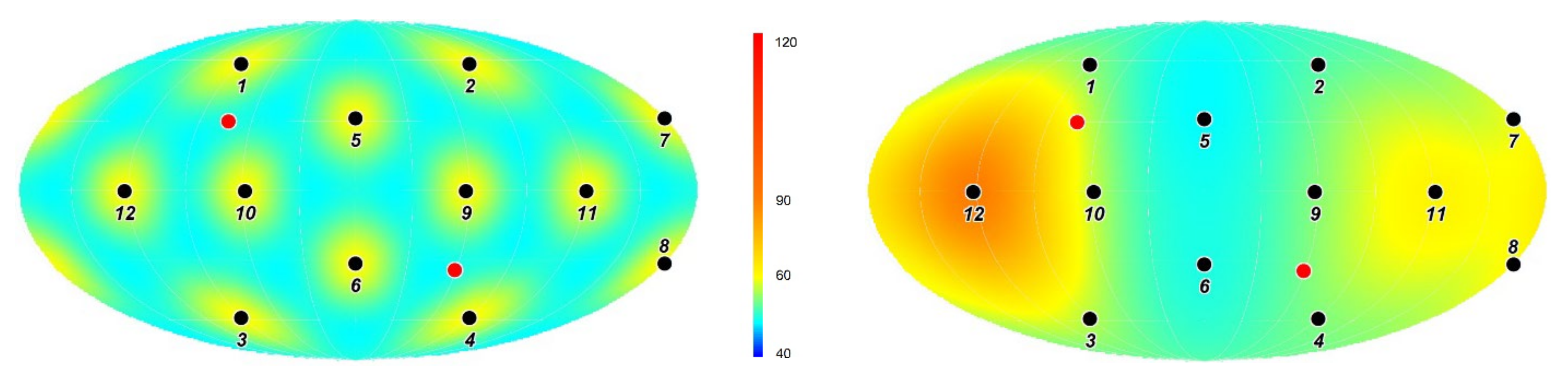
Spatial distribution of NH3 after 100 Martian years: “factory” alternative variant (left), “asteroid” alternative variant (right).
Figure 15.
Spatial distribution of NH3 after 100 Martian years: “factory” alternative variant (left), “asteroid” alternative variant (right).
Figure 16.
Average temperature rise on Mars over 100 simulation years after the initial event.
Figure 16.
Average temperature rise on Mars over 100 simulation years after the initial event.
Figure 17.
Standard deviation of the temperature rise on Mars over 100 simulation years after the initial event.
Figure 17.
Standard deviation of the temperature rise on Mars over 100 simulation years after the initial event.
Figure 18.
Percentage of Mars area with an average temperature above −25 °C (habitable area) and above 0 °C (biosphere).
Figure 18.
Percentage of Mars area with an average temperature above −25 °C (habitable area) and above 0 °C (biosphere).
Figure 19.
Tempe: 100 GT “asteroid” (top); 1.5 MT “factory” (bottom) (after 100 Martian years).
Figure 19.
Tempe: 100 GT “asteroid” (top); 1.5 MT “factory” (bottom) (after 100 Martian years).
Figure 20.
Temperature increase after 100 Martian years: “factory” alternative (left), “asteroid” alternative (right).
Figure 20.
Temperature increase after 100 Martian years: “factory” alternative (left), “asteroid” alternative (right).
Figure 21.
Average temperature rise on Mars over 100 simulation years after the event.
Figure 21.
Average temperature rise on Mars over 100 simulation years after the event.
Figure 22.
Standard deviation of the temperature rise on Mars over 100 simulation years after the event.
Figure 22.
Standard deviation of the temperature rise on Mars over 100 simulation years after the event.
Figure 23.
Percentage of Mars area with an average temperature above −25°C (habitable area) and above 0 °C (biosphere).
Figure 23.
Percentage of Mars area with an average temperature above −25°C (habitable area) and above 0 °C (biosphere).
Figure 24.
Twelve 8.3 GT “asteroids” (top), Twelve 125 kT “factories” (bottom) (after 100 Martian years).
Figure 24.
Twelve 8.3 GT “asteroids” (top), Twelve 125 kT “factories” (bottom) (after 100 Martian years).
Figure 25.
Spatial distribution of NH3 after 100 Martian years: “factory” alternative variant (left), “asteroid” alternative variant (right).
Figure 25.
Spatial distribution of NH3 after 100 Martian years: “factory” alternative variant (left), “asteroid” alternative variant (right).
Table 1.
Parameters for greenhouse gasses [
20,
21,
22,
23].
Table 1.
Parameters for greenhouse gasses [
20,
21,
22,
23].
| Gas Name and Chemical Formula | Carbon Dioxide—CO2 | Ammonia—NH3 | Methane—CH4 | Freon (CFC) |
|---|
| gray opacity (for 0.0001 bar of gas) | 0.029 | 0.504 | 0.039 | 0.007 |
| gray opacity (for 0.01 bar of gas) | 0.081 | 2.199 | 0.139 | 0.440 |
| eddy diffusion (for 150 K) | 3.19 × 10⁻² | 4.79 × 10⁻² | 4.07 × 10⁻² | 2.23 × 10⁻² |
| eddy diffusion (for 150 K) | 9.03 × 10⁻² | 13.5 × 10⁻² | 11.5 × 10⁻² | 6.32 × 10⁻² |
Table 2.
Parameters for selected points.
Table 2.
Parameters for selected points.
| Point/Parameters (1 sol) | Hellas | Tempe |
|---|
| LAT/LONG/H | −34.595/58.982/−6894.5 | 30.303/−73.236/−210.9 |
| Temperature (K) | 197.8 | 165.6 |
| Pressure (Pa) | 1106.2 | 591.4 |
| CO2 content (kg/m2) | 3.21 | 1.73 |
| Zonal wind (m/s) | 1.9 | 3.4 |
| Meridional wind (m/s) | −1.1 | −3.2 |
Table 3.
Energy costs for launching the nuclear bomb into asteroids from Kuiper belt.
Table 3.
Energy costs for launching the nuclear bomb into asteroids from Kuiper belt.
| Asteroid Mass | Missions qty. | Energy of Single Bomb | Single Rocket Fuel Energy | Total Energy |
|---|
| 100 (GT) | 1 | 4500 × 1015 (J) | 1.4 × 10⁹ (J) | 4500 × 1015 (J) |
| 8.3 (GT) | 12 | 375 × 1015 (J) | 5.5 × 10⁸ (J) | 4500 × 1015 (J) |
Table 4.
Energy costs for partial vaporization of asteroids from Kuiper belt.
Table 4.
Energy costs for partial vaporization of asteroids from Kuiper belt.
| Asteroid Mass | Missions qty. | Energy of Single Engine | Single Rocket Fuel Energy | Total Energy |
|---|
| 100 (GT) | 40 | 157.68 × 10¹⁵ (J) | 5.5 × 10⁸ (J) | 6307 × 1015 (J) |
Table 5.
Energy required for greenhouse gasses production on Mars.
Table 5.
Energy required for greenhouse gasses production on Mars.
| Amount of CFC per Sol | Number of Factories | Time of Production | Total Energy Required |
|---|
| 125 (kT) | 12 | 95 × 668 (sol) | 91.4 × 10¹² (J) |
| 1500 (kT) | 1 | 95 × 668 (sol) | 91.4 × 10¹² (J) |
| Publisher’s Note: MDPI stays neutral with regard to jurisdictional claims in published maps and institutional affiliations. |
© 2022 by the authors. Licensee MDPI, Basel, Switzerland. This article is an open access article distributed under the terms and conditions of the Creative Commons Attribution (CC BY) license (https://creativecommons.org/licenses/by/4.0/).


