Abstract
One of the bottlenecks of autonomous systems is to identify and/or design models and tools that are not too resource demanding. This paper presents the concept and design process of a moving platform structure–electric vehicle. The objective is to use artificial intelligence methods to control the model’s operation in a resource scarce computation environment. Neural approaches are used for data analysis, path planning, speed control and implementation of the vision system for road sign recognition. For this purpose, multilayer perceptron neural networks and deep learning models are used. In addition to the neural algorithms and several applications, the hardware implementation is described. Simulation results of systems are gathered, data gathered from real platform tests are analyzed. Experimental results show that low-cost hardware may be used to develop an effective working platform capable of autonomous operation in defined conditions.
1. Introduction
Modern mechatronic systems require elastic tools for design, control and data analysis. Often, significant challenged arise due to data uncertainty, robustness against disturbances and model-free modeling caused by real data processing and problems with mathematical descriptions of issues. Neural networks seem to be an appropriate and useful solution to a number of the issues encountered. Today, due to the availability of efficient programmable devices and algorithms presented in the literature, interest in implementation of neural processing in electric vehicles is also increasing [1,2,3]. This paper describes the application of modules based on different types of neural networks in a real model of a moving platform.
Presently autonomous vehicles are becoming increasingly popular. Using such vehicles in industry and testing the systems in real-life applications is becoming more commonplace. Unmanned Aerial Vehicles (UAVs) have been developed for monitoring hazardous zones such as minefields or remote and inaccessible locations. The autonomous vehicles are also being tested for use in public areas; tests of unmanned shuttle buses or surveillance vehicles have been conducted. In those cases, the zone was strictly defined, and the vehicles had to react to changing conditions and obstacles. Autonomous platforms for delivery and warehouse movement are also being tested also under development [4,5,6,7,8].
The data processing in autonomous vehicles should be based on human brain functionality because there is no possibility to predict all situations and issues while designing a control system. There is a need to use control structures to adapt to the driving environment and give the vehicles the capacity to infer commands based on sensor data and gathered knowledge without driver (or external user) assistance. The environment, laws and driving habits are different all around the world, and it is impossible to create a universal database of driving rules (Figure 1). The autonomous self-learning cars are also supposed to increase safety in traffic, improve vehicle flow and reduce energy consumption [9,10,11]. According to SAE J3016, classes of vehicle automation are precisely defined. In Classes 4 and 5 of SAE J3016, the system is responsible for driving, reacting to obstacles and handling emergency situations [12]. The difference between them is the operational domain. While Class 5 vehicles are supposed to react in every environment, Class 4 vehicles are only autonomous in defined driving conditions [13]. While higher classes indicate novel autonomous systems which are still under development, Classes 0–3 are already implemented in the vehicles available on market. Even though, Class 0 represents vehicles without autonomous skills, the sensor systems may be implemented to gather environmental data and display proper information for drivers. The higher classes introduce the ability to interpret sensor data in particular driving tasks, such as driving in parking lots or lane assistance. However, the driver remains the main supervisor; the systems are only their assistants [14].
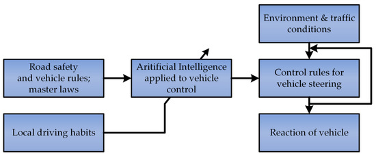
Figure 1.
The concept of the data processing based on artificial intelligence in the autonomous vehicle.
The increase in popularity of neural networks in a variety of applications is observed in the literature. Several existing applications can determine the sizes and structures of neural networks. Neural networks may be used as controllers, estimators and classifiers, which makes them very popular tools in the design of control structures [15,16,17,18,19,20,21]. With the development of hardware and high demand, new neural structures need to be developed. Deep learning convolutional networks are the most powerful structures which have overcome the fully connected multilayer perceptron neural networks in data analysis and image classification [22,23]. A comparison of the efficiency shows that the input data for deep networks can be unprocessed; however, the demands in terms of hardware are incomparable (higher). While multilayer perceptron neural networks are usually implemented with DSP processors and FPGA matrices [24,25], the deep neural structures require special processing units or multi-core processors. It can be seen that the implementation of neural classifiers on powerful GPUs is also becoming more popular [26]. Nevertheless, this research attempts to implement different neural structures with low-cost hardware. The proper design and applied simplification are described in detail to run a NN on an 8-bit microcontroller. The last part of the paper describes a simple deep network which was trimmed to work with an inexpensive specialized coprocessor in an RISC-V processor.
The goal of this work was to design and create a model of an autonomous platform enabled for driving in a defined environment using low-cost hardware. Because of the restricted driving conditions (of Class 4), some assumptions can be defined [27]. The first design problem was related to potential of implementing Artificial Intelligence (AI) algorithms on Arduino development boards. The control structure utilizing neural computation was supposed to collect sensor data and commands to develop a self-learning path planner. The neural controller should cooperate with the neural image classifier. The control commands should be accessible in the microcontroller system. The control structure should be able to use neural computing for gathering sensor data and operate the hardware, for example DC motors. This paper not only provides a general review, but also a detailed descriptions of design, used hardware and test results.
A microcontroller system consisting of three development boards was designed (Figure 2). The main controller was implemented in Arduino MEGA 2560. The main advantage (in this project) of the board is the variety of accessible input/output ports and multiple communication modules (e.g., 4 UART serial ports). The main device was responsible for data collection, distance estimation and commands processing. Motor controllers were driven by Arduino UNO reacting to commands received by UART. Drive encoders and current sensors were wired directly, enabling low-level control. The vision system was developed with the most powerful development board, Sipeed Maix Bit. It can control the camera and perform neural object classification. An in-vehicle network was created by establishing a connection between the mentioned boards using UART communication. To reduce complexity of data transfer, simple commands were defined.
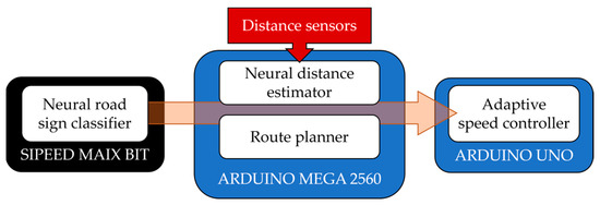
Figure 2.
The scheme of a microcontroller system of the analyzed platform.
This paper consists of seven sections. After the introduction presenting main issues related to the models of electric vehicles and indicating the main concept of the work (details of the autonomous model based on neural data processing), the neural network applied for the analysis of data from distance sensors is described. Next, the feed-forward neural network applied as reference command manager is proposed. The following section deals with the adaptive speed controller implemented for the DC motors. Additionally, a deep learning technique is used for images classification. The points mentioned above complete the details of the neural modules used in the real model of the vehicle. Thus, a subsequent part of the manuscript focuses on the construction of the real platform. Then, tests and short concluding remarks are shown.
2. Neural Distance Estimator
The platform was equipped with two optical distance sensors mounted on the front. Their mission was to measure the distance to the nearest obstacle. The first sensor was an analog optical sensor-Sharp GP2Y0A41SK0F (whose measurement range is 0.04–0.30 m). The second one was a digital sensor VL53L0X (with a proper working distance up to 2.50 m). Because of the optical technology, it was assumed that real results may change due to lighting conditions and the surface type. The tests were conducted to compare results obtained with the sensors mentioned above with actual distance to obstacle. All sensors were placed on a stationary support enabling the researchers to take all measurements without any accidental displacement. The results obtained during the test are shown in Figure 3. It should be noted that the achieved values do not define properties of the tested sensors but introduce an assessment of the implementation possibility in the described robot (in specific working conditions).
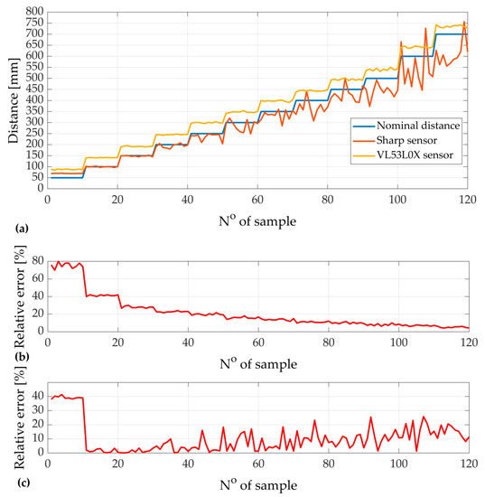
Figure 3.
Measurement tests results: (a) comparison of applied sensors; (b) relative error for VL53L0X sensor; (c) relative error for Sharp sensor.
It should be noted that while VL53L0X sends an explicit result in millimeters via the I2C protocol, the output of the Sharp sensor is the voltage level corresponding to the distance. After calculations of the voltage VADC (using ADC—Analog to Digital Converter), the distance has to be calculated using Equation (1) [28,29,30,31]. The formula seems to be unsuitable for simple 8-bit controllers because of the fractions, exponentiation and multiplications (according to observations, it takes more than 1 ms to compute).
where ln is the distance to the obstacle, and VADC is the voltage measured and calculated by the ADC module.
The input vector of the designed neural structure consists of an ADC value and a VL53L0X sensor response. For training purposes, the real reference value of the distance was the target. A neural network structure was created and trained in Matlab software [32]. Because of the fact that the neural network was designed to be implemented in a low-cost microcontroller system (i.e., Arduino), two hidden layers (with two nodes each) were implemented (Figure 4). For weight optimization, the Levenberg–Marquardt algorithm was used [33]. To implement the trained neural structure, it was necessary to deactivate the preprocessing of input data in Matlab. By default, normalization of the input vector is computed as follows:
where and are max and min values of the target matrix, respectively, and xmax, xmin are maximum and minimum values of the input vector, respectively.
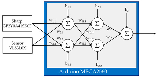
Figure 4.
The structure of the neural distance estimator.
Unfortunately, without any configuration, The normalization process was computed for every input row independently [34]. However, when the preprocessing was disabled, it was possible to easily implement the structure as a matrix calculation on direct results obtained by the sensors.
Because of already mentioned hardware limits, a linear activation function was chosen. Weights and bias values were extracted in matrix forms and saved in Adruino MEGA 2560. The MatrixMath library was utilised to generate results by conveniently typing direct functions instead of complex for loops. The neural distance estimator was tested, and results are shown in Figure 5. Not only was improvement in accuracy observed, but also time efficiency was obtained. The reason was the simplification of the calculation–only summing and multiplying are needed as shown in Equations (3)–(5) below:
where are the outputs of the first, the second and the output layer, respectively; X is the input vector, IW is the matrix of input weights, LW is the matrix of the hidden layer weights, OW is the matrix of the output layer, and are the vectors of the biases of input and the hidden layer.
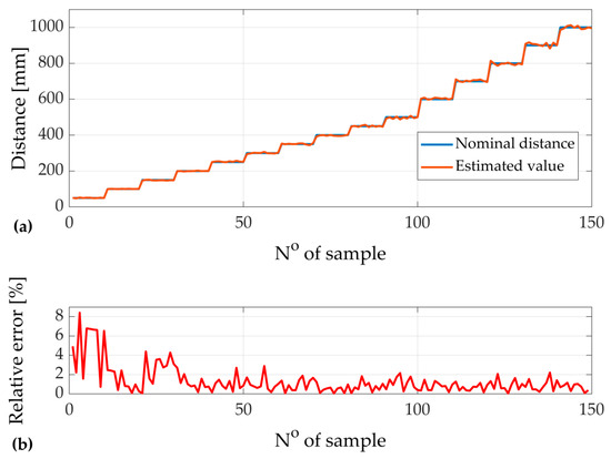
Figure 5.
Results of neural distance estimator: (a) comparison of estimator response and nominal distance; (b) relative error value.
Table 1 presents a comparison of calculation times. Application of the neural model leads to about twice as fast calculations. The precision of the final values is also much higher. In Table 2, the calculated values of relative errors are given [35]. The average relative error for the neural distance estimator is only 1.23%, while the Sharp sensor has an 11.28% relative error, and 17.7% for the VL53L0X sensor. The value of the relative error was reduced to only 0.1 of initial values.

Table 1.
Comparison of computing times for different methods of distance calculation.
Table 2.
Values of relative errors for the sensors and the estimator.
3. Self-Learning Neural Path Planner Applied to the Platform
The platform was equipped with an SD card module. It allows the platform to collect sensor data and control commands. This allowed us to save samples to be used later as training data for the neural network used for this task. As an example, a short test ride in a closed area with one obstacle was conducted (Figure 6). Based on the gathered data and expected commands, the model was trained [36]. The input vector consisted of sensor data, previous samples (for better representation of the dynamic state changes of the position of the vehicle) of commands and measured distances:
where vr is the speed of right wheels, vl is the speed of left wheels, lf is the distance to an obstacle in front of the model, lr is the distance to the wall on the right side, ll is the distance to the wall on the left side, k is the number of the sample.
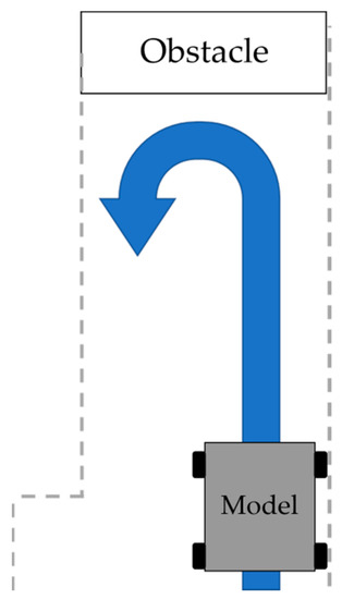
Figure 6.
Trajectory assumed for test performed for training data gathering.
The output of the structure was a two-row vector of forcing speeds for left and right wheels. At this point in the work, implementation of the MultiLayer Perceptron (MLP) with linear activation functions was proposed. As in the previous section, the adaptation of internal coefficients was performed using the Levenberg–Marquardt algorithm. In Figure 7, both target control signals and neural planner response are presented. It is worth indicating that the transients of reference speeds of the wheels are similar for both types of control loop. The response of the neural path planner is smoother as in case with no quantized values. Such a ‘soft’ reference signal is easier to reproduce and may lead to smaller overshoots obtained by the speed controller. As it can be seen in Figure 7, an insignificant difference in desired speeds of the left and the right wheels was observed while the neural controller was applied. During the performed test, it did not affect the desired path. The most visible disadvantage of the neural structure was the delay that was observed. The reaction was delayed by one sample. Nevertheless, it is possible to apply the designed neural planner in the control structures of vehicles where an automatic control is the most important observed feature and may be neglected. Moreover, after additional pre-processing (shift of the output samples relative to input values) of the measured training data, the mentioned delay can be eliminated.
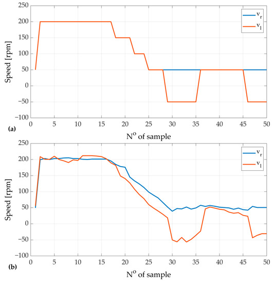
Figure 7.
Comparison of reference speeds: (a) standard commands (defined by user); (b) neural path planner response.
4. Neural Speed Controller
The platform was propelled with four DC motors grouped into two pairs (for left and right side). To perform turns, a separate control of left and right wheels was necessary [37,38]. To ensure steering of the vehicle, two separate speed controllers should be implemented. Each pair of DC motors was powered with a driver (based on the H-bridge) equipped with an encoder. The code used for calculation of the speed controller was implemented in Arduino Uno.
When analyzing the published literature that describe electric drives of vehicle powertrains, correct functioning under dynamic states and robustness against disturbances seem to be important requirements. Thus, the significant problem deals with the construction of mentioned drive. Because of the fact that the electric drives are always merged with mechanical structures such as gearboxes, couplings or shafts, additional disturbances and variable state oscillations were observed. Those phenomena are highly disruptive, not only for safety reasons, but also because of increased possibilities of damage; precision of control is also difficult to ensure.
Due to the reasons given above, a vehicle adaptive neural speed controller was implemented. The most important advantage of such a structure is the possibility of autonomous adaptation to changing working conditions [39,40]. Firstly, the tests were conducted in Matlab/Simulink based on the model obtained with the System Identification Toolbox. The structure of the adaptive control with the reference model was proposed (Figure 8). The aim of the reference model is to calculate the error based on the modified reference signal and apply the information as feedback for an adaptation algorithm. Such a model provides the possibility to correct the reference signal if forced dynamics exceed motor features. For simulation purposes, the following transfer function was used:
where is the damping coefficient and is the resonant frequency.
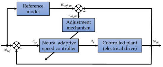
Figure 8.
Neural adaptive control structure with reference model.
The parameters of the reference model can shape the dynamics of the input signal. The conversion of the external waveform was applied to match the performance of the controlled plant. If the difference in dynamics of both the out variable state (speed) and the reference signal is significant, the adjustment mechanism cannot find the steady values of the controller coefficients.
A neural-like structure of speed controller with six tunable weights was tested (Figure 9). The output value of the controller can be obtained using the expression below (generalized for a variable number of trainable weights):
where is the vector of input values, is adaptable weights, and f() is the activation function.
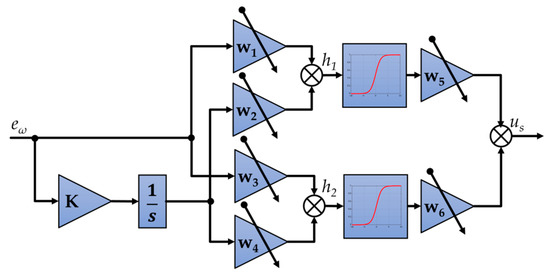
Figure 9.
Structure of neural adaptive speed controller.
The given description is valid for the model where additive biases are omitted, input vector consists of J elements, and I is number of neurons in the output layer. In practice, for adaptive controllers (with online training), omitting bias values is common. If the assumption mentioned is not taken into account, the general description of the neural controller can be given as below:
where is the output activation function, is the biases of the output layer, is the activation function of the input layer, is the bias values of the input layer, and is the vector of the controller input values.
As can be seen in the scheme of the controller (Figure 8), the input vector of the structure consists of error values (it is calculated as a difference between reference values and measured speed), the integration of successive values is also introduced as:
where is the reference speed, is the measured speed, and K is the input gain coefficient.
The general idea of the controller is to adapt the values of network weights (in the presented controller, the – coefficients) during operation of the motor. This online computation process is performed in parallel to the main neural network. The main goal is to minimalize the value of the cost function defined as follows:
where is the value of o-th output of neuron, is the demanded value of o-th output, and O is the number of considered outputs.
The basic idea of adaptation is described with the following:
where is ij-th the controller coefficient value in the k-th step of the simulation, is ij-th the correction value calculated according to the equation presented below (it corresponds to a gradient-based optimization method):
where f is the activation function, is the adaptation coefficient, is the output of the i-th node, x, y are the input and output values, and is the error between demanded and real output.
According to the literature, the given adaptation algorithm can be simplified. The first element of Equation (14) equals zero because of the lack of the following connections, while the second part can be omitted for internal neurons, as they are not directly affected by the output yo. Additional details of the speed control algorithm are presented in [41]. After theoretical considerations, some similarities to adaptive pinning control can be noticed (the update of parameters, convergence analysis, etc.) [42].
The simulation test of the structure (Figure 10) was conducted with a square signal (amplitude 150 rpm and frequency of 0.2 Hz) applied as a reference trajectory (Figure 10a). Such a trajectory represents electric drive reversals and also ensures better visibility of the adaptation process. At the beginning, oscillations and overshoots are visible; however, after every repetition the inaccuracies are reduced. Efficient recalculation of weights can be observed in Figure 10b. Random values of the internal parameters of the controllers were assumed. The weight values are continuously modified in the recalculation process. The most significant changes occur at the reference speed changes. However, after a certain period of time, the system stabilizes. The achieved results were obtained for the control structure realized with the adaptation coefficient and integral part coefficient K = 5.
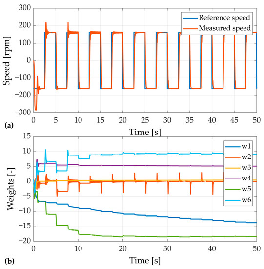
Figure 10.
Adaptation process of the speed controller: (a) transients of speed; and (b) weights values.
Simulations confirm the efficiency of the neural adaptive speed controller. The most important advantage of the structure is the lack of a necessity to perform initial tuning of the controller. The adjustment is an automated process and is performed online during operation of the motor (Figure 10b). The inaccuracies in measured speed transient are mostly visible only at the beginning of motor operation. It can be assumed that adaptation works correctly, and all unwelcomed disturbances are quickly damped.
5. Neural Road Sign Classifier
The vehicle was also equipped with an RGB camera (on the front of the platform). The images were processed by a Sipeed Maix Bit microcontroller board. It is a specialized microcontroller with a V-RISC dual core microprocessor. The dedicated neural processing unit KPU enables the board to work as a real-time image analyzer. It is capable of operating with 3 × 3 kernel matrices and any activation function. This enables the system to work as a real-time vision system. In UAVs, vision systems may detect obstacles, trace the lines, read QR or bar codes. In case of autonomous vehicles, a vision system should be also able to detect traffic information from existing infrastructure (for example traffic lights or road signs) [43,44,45,46]. In the designed structure, the vision system was implemented for road sign classification. After analysis of the object, the suitable command is propagated via the UART module to the main controller to interrupt current ride and perform pre-programmed behavior (Figure 11). In Table 3 the list of signs, corresponding commands and designed platform behavior is given.
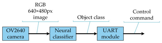
Figure 11.
Scheme of vision system processing.
Table 3.
The rules assumed for the neural classifier.
For neural image classifier, a deep neural network was used (Figure 12). The idea of such a structure is to use a raw RGB image, which is represented with three matrices, as input [47,48]. Then every matrix, corresponding to one color (red, blue, or green), is involved in convolution. The input matrices are convolved with the kernel matrix to create new matrices with different number of cells. In the convolutional layer, the kernel biases are trainable parameters. The kernel size for the convolution with the input data can be adapted to the designed functionality. Then, the matrices are downsampled with a moving pooling window to create feature matrices (maps). As shown in Figure 12, max() function was applied in tests. Another popular pooling function is average() which could return the mean value of the cells in a window. It is considered as a blurring data processing agent. In the application shown in Figure 12, the feature maps are the matrices filled with filtered max values of convolutional layers. The convolution and pooling process may be repeated to create small matrices which are the input to a fully-connected network. Inputs are called “deep matrices”, where only features (e.g., edges) are extracted. The fully-connected layer consists of an MLP neural network; it can classify or detect objects on the basis of input features. It is worth indicating the difference between classification and detection. The classifier only returns the membership of the object to classify and the probability of such prediction, while the detector response consists of a class, probability, positions and size of the bounding box imposed over the object (Figure 13) [49,50].
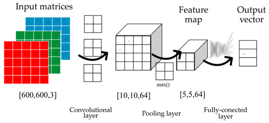
Figure 12.
Idea of deep learning data processing.
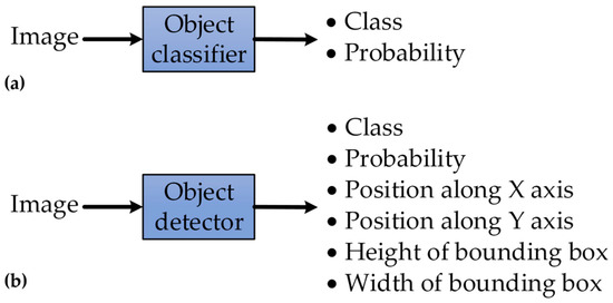
Figure 13.
Comparison between classifier and detector: (a) inputs and outputs of object classifier; (b) inputs and outputs of object detector.
For the model of the vehicle, the classifier was developed using an aXeleRate structure based on the Keras library. The structure and the library utilize TensorFlow neural models, which can be adjusted and trained using a previously prepared dataset [51,52]. For training purposes, the set of road signs images had to be prepared. According to the literature, the diversity of training data is necessary to obtain good efficiency [53,54]. The photos were taken with different cameras in different lighting conditions and with different angles. Moreover, the datasets were extended by creating copies of the images with adjusted saturation and brightness, blur or noise added. Not only were additional samples created, but also better diversification was obtained. Images with cropped, rotated, distorted or partially covered signs were also included. Every image was then cropped to a square of 150 × 150 pixels. The dataset was saved in directories with names of expected classes. If an object detector was trained, the images were also equipped with labels indicating the position of the object. That created additional xml files with the position and size of the bounding box. After collecting and managing the training data, a MobileNet algorithm was chosen for training the TensorFlow classifier structure [55,56]. The applied structure uses 150 × 150 × 3 input matrices, then 5 convolutional layers resulting in 16, 32, 64, 128, 256 and 256 matrices successively. The fully-connected network had 4 layers with 256 inputs and 200, 150 and 100 neurons respectively (Figure 14).
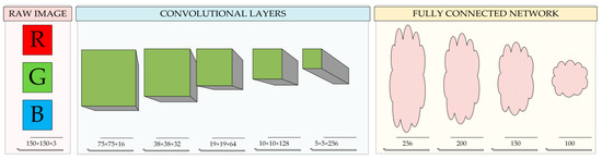
Figure 14.
Structure of deep neural network image classifier.
In the MobileNet structure, convolutional layers not only convolute the matrices but also normalize the data with ReLU (Rectified Linear Unit) activation function:
where is the input value for ReLU function.
The training was conducted on the Google Colab system with Tesla P100-PCIE16GB GPU that enables researchers to use GPU acceleration and significantly reduces computing time [57]. The aXeleRate structure was trained during 5000 epochs; additionally, the early stopping option was enabled and an embedded dataset extension (by noise adding with dropout value 0.5 was activated) was used. After the training, the TensorFlow model had to be compiled into an optimized form of the TensorFlow Lite model. The main difference between the mentioned models deals with weight quantization (the Lite version uses 8-bit precision) [58]. It enables models to work in real time on neural computing supporting microcontrollers. The MobileNet structure was chosen because of good classification efficiency [59,60]. The net structure was originally developed by Google in 2017, and it was designed especially for mobile applications [61]. It is a universal structure that can be trained and employed for detection, classification and segmentation tasks. The main advantage of using such a structure is the limited number of trainable parameters. The deep-learning structure consists of both a convolutional and a fully-connected network. However, the reduced number of parameters was obtained by considering the convolution kernel height and width independently. The kernel can be obtained after matrix multiplication of two vectors. The feature map is obtained during a two-step convolution (depthwise separable convolution) process. At the beginning, a standard 3 × 3 kernel is used to obtain reduced data with the same depth. Then, a 1 × 1 kernel is applied to take depth into account. Such an approach gives the possibility for faster data processing in mobile devices (because of smaller kernels) and noticeably reduces the number of parameters.
The other models were also tested on limited datasets to compare efficiency, training time, number of trainable parameters and file size (Table 4). The classification efficiency was calculated according to the following formula:
where P is the classification efficiency [%], nOK is the number of correctly classified images, and ndt is the number of images in the dataset.
Table 4.
Comparison of neural classifiers.
Results gathered in Table 4 indicate significant differences between the tested deep-learning structures. It is worth indicating that the quickest training took only 1 min (resulted in efficiency of 40%) and the longest required nearly half an hour (did not increase precision with overall efficiency of only 26.7%). MobileNet structures are characterized with the best efficiency (higher than 73%) and reasonable training time (less than 5 min). Because implementation in a low-cost microcontroller is taken into account, the size of the model is also important. The smaller the number of parameters, the smaller the size of the output file is. As it can be seen, the model described with the smallest file (with only about 315,000 parameters) works much better than oversized structures.
A novel approach for distance estimation was also proposed and tested. The idea is based on image analysis. An additional one-class detector was trained to analyze the “STOP” sign. Taking the assumption that all objects have identical size, it is possible to estimate the distance from the sign using the vision system. The information can be obtained by comparing the width of the bounding box and class name with an index in the lookup table (Figure 15a). The relations between distance and the size of the bounding box can be established for known conditions of operation and saved. Using experimental results obtained with a 640 × 480 camera, the lookup table was proposed (Table 5). The experiment was performed for a detector implemented in a microcontroller (Figure 15b), and the bounding box size was the direct result. Such an approach may lead to a reduction of the distance number of sensors or fault-tolerant control (without additional sensors).
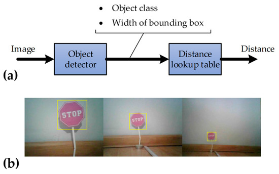
Figure 15.
Application of vision system for distance estimation: (a) flow diagram of proposed structure; (b) images of “STOP” sign’ analyzed during the experiment.
Table 5.
Proposed lookup table for experimental data.
6. Real Platform
The described microprocessor system was mounted on a double-deck metal chassis (Figure 16). It makes it possible to gather each element of system tidily. On the bottom deck, DC motors with servos, encoders and Arduino Uno were placed. On the second level, the main controller (Arduino MEGA 2560) was mounted longitudinally. The supports for two side-sensors were designed and created with Fused Deposition Modeling (FDM) technology. The optical distance sensors were mounted above each other at the front of the platform. The vision system, with a Maix Bit development board and the camera, was rigidly fixed to the PCB, which was mounted with additional elements (also created with the 3D print) on top of the front sensors. Arduino boards and DC motors were powered with stabilized voltage (6 V). It was ensured with the DC/DC converter supplied with two 18,650 Li-ion batteries. The sensors were powered directly from the development boards. The platform was also equipped with a USB powered battery charger. The Maix Bit board and the camera were powered from an external power bank using a USB-C cable. The modular structure gives the possibility to expand the system with additional elements (e.g., accelerometers or GPS receivers) in further development.
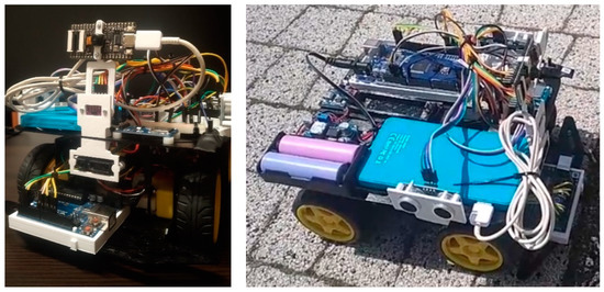
Figure 16.
The real structure of platform.
Finally, the functional test was performed to verify assumptions, results of simulations and confirm feasibility of autonomous driving of the platform. The test drive was performed outside, to reduce noisy data from the low-cost sensors caused by unsuspected reflections. Firstly, the autonomous control system was tested (Figure 17). The platform was placed in front of a wall and two boxes forming an alley. It is worth indicating that one was white and the second was black. It was intended as an additional test of a neural distance estimator (utilizing optical sensors). As it can be seen on the presented illustration, the system works correctly, the platform avoided crashing into obstacles and moves according to reference (expected) path trajectory. During the initial test, data from sensors and control commands were saved on an SD card. Next, the control system was switched to reading mode. The platform was placed in an open area, and the previously predefined trajectory was perfectly reproduced.
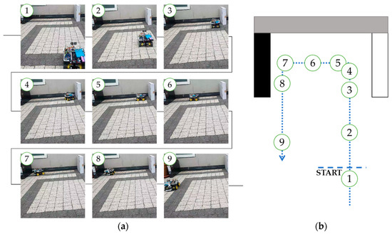
Figure 17.
Subsequent frames presenting functional test of the platform: (a) real model view; (b) graph of the trajectory.
The last test was also executed in an open area. The control system was switched to autonomous driving mode. The goal of this trial was to confirm the effectiveness of the neural road sign classifier and the accuracy of the feedback loop of that system. The “STOP” sign was placed in front of the platform, a couple meters distant from the starting point. After switching on, the model accelerated, then stopped before the object and set off. The evaluation was positively passed; the construction of the platform and the applied neural control systems works correctly.
Further research concerning the design of the platform will be conducted. The power for the microcontroller system is planned to be delivered from an alternative renewable energy source, such as photovoltaic panels. Such a design is especially beneficial for small delivery robots operating in open areas. However, safety has to be ensured first, so the energy consumption of every element will be verified. As the vision system is also independent in case of energy source and is implemented on the most powerful microcontroller, the preliminary energy usage was measured with a simple USB power meter.
7. Conclusions
The paper presents a successful design of a microcontroller system of a platform with implemented artificial intelligence elements. For this purpose, the following components/issues were based on neural networks: movement of the platform, sensor data gathering, autonomous driving basing on commands from the control system and the neural vision system. Several parts of the system were described. Then, a complete, final form of the vehicle was presented. This work confirms the possibility of the application of neural computing with simple hardware. The following remarks can be drawn from the project:
- Direct mathematical modeling was minimized during the design process of the vehicle. It leads to simplification. However, according to the data representation of the issue (for each analyzed task), the specificity of the object can be taken into account (parameters, nonlinearities, disturbances, etc.).
- Multilayer perceptron neural networks and deep neural networks can be utilized in autonomous vehicles used with low-cost hardware (programmable devices).
- The novel idea of the neural distance estimator allows us to enhance the sensing precision of results. Not only is measurement error minimalized, but computing time is also optimized. That is an advantage in the applications such as autonomous vehicles, where reaction should be immediate. Taking into consideration that the relative error was reduced to only ~1.5% using cheap model sensors, even better results may be obtained utilizing more sophisticated hardware.
- The analyzed structure of neural adaptive speed controller confirms that online tuning of a speed controller is efficient. The main advantage of the control structure is the fact that the transient of speed does not contain overshoots and oscillations after the few adaptation steps. It is worth indicating that the adaptation is an automatized process based on the response of the model.
- Convolutional networks can be easily implemented as neural object classifiers utilizing TensorFlow libraries and additional training features such as aXeleRate libraries. The best classification efficiency for the tested dataset and road sign recognition problem was obtained with a MobileNet neural model.
- A vision system with neural data computing can be implemented with low-cost hardware. A fully working system was achieved with a Sipeed Maix Bit board and OV2640 camera. Because of the variety of supported communication modules, the vision system may be easily connected with most control systems available in the market. The utilized hardware cost can be calculated at about USD 40.
- The design and implementation of this project has proven that low-cost hardware may be used to develop an effective working platform capable of autonomous operation in defined conditions. Such platforms may be implemented in industry as in-plant deliveries. The system may be easily equipped with a wireless transmission module such as Bluetooth or Wi-Fi to send data to a cloud, enabling the smart management of a swarm of platforms.
- Further research will be focused on energy consumption optimization to make the platforms independent of external power sources and to reduce maintenance time required for charging. Alternative renewable energy sources are considered to be added.
Author Contributions
Conceptualization, M.M., J.-R.T. and M.K.; methodology, M.M., J.-R.T. and M.K.; software, M.M.; formal analysis, J.-R.T. and M.K.; writing—original draft preparation, M.M., J.-R.T. and M.K.; writing—review and editing, M.M., J.-R.T. and M.K.; visualization, M.M.; supervision, M.K. All authors have read and agreed to the published version of the manuscript.
Funding
This research received no external funding.
Data Availability Statement
Not applicable.
Conflicts of Interest
The authors declare no conflict of interest.
Abbreviations
| ADC | Analog to Digital Converter |
| AI | Artificial Intelligence |
| DC | Direct Current |
| FDM | Fused Deposition Modeling |
| FPGA | Field-Programmable Gate Array |
| GPS | Global Positioning System |
| GPU | Graphics Processing Unit |
| I2C | Inter-Integrated Circuit |
| MLP | Multilayer Perceptron |
| SAE | Society of Automotive Engineers |
| UAV | Unmanned Aerial Vehicle |
| UART | Universal Asynchronous Receiver-Transmitter |
| Symbols | |
| distance to obstacle | |
| voltage level measured with ADC | |
| element of target matrix | |
| general symbol of input value | |
| general symbol of matrix of output values | |
| general symbol of matrix of input values | |
| weight of i-th neuron node in j-th layer | |
| lf | distance to an obstacle in front of model |
| lr | distance to an obstacle on right side |
| ll | distance to an obstacle on left side |
| k | number of samples. |
| damping coefficient | |
| resonant frequency | |
| speed error | |
| model reference speed error | |
| reference speed | |
| model reference speed | |
| control signal | |
| measured speed of motor | |
| speed controller input vector | |
| integral gain | |
| bias of i-th neuron node in j-th layer | |
| correction value of weight | |
| general symbol of output value | |
| speed of left wheels | |
| speed of right wheels | |
| input of ReLU function | |
| classification efficiency | |
| number of correctly classified samples | |
| number of samples in dataset |
References
- Chen, Z.; Yang, C.; Fang, S. A Convolutional Neural Network-Based Driving Cycle Prediction Method for Plug-in Hybrid Electric Vehicles with Bus Route. IEEE Access 2019, 8, 3255–3264. [Google Scholar] [CrossRef]
- Caban, J.; Nieoczym, A.; Dudziak, A.; Krajka, T.; Stopková, M. The Planning Process of Transport Tasks for Autonomous Vans—Case Study. Appl. Sci. 2022, 12, 2993. [Google Scholar] [CrossRef]
- Vodovozov, V.; Aksjonov, A.; Petlenkov, E.; Raud, Z. Neural Network-Based Model Reference Control of Braking Electric Vehicles. Energies 2021, 14, 2373. [Google Scholar] [CrossRef]
- Bołoz, L.; Biały, W. Automation and Robotization of Underground Mining in Poland. Appl. Sci. 2020, 10, 7221. [Google Scholar] [CrossRef]
- Rahman, A.; Jin, J.; Cricenti, A.; Rahman, A.; Palaniswami, M.; Luo, T. Cloud-Enhanced Robotic System for Smart City Crowd Control. J. Sens. Actuator Netw. 2016, 5, 20. [Google Scholar] [CrossRef] [Green Version]
- Amicone, D.; Cannas, A.; Marci, A.; Tortora, G. A Smart Capsule Equipped with Artificial Intelligence for Autonomous Delivery of Medical Material through Drones. Appl. Sci. 2021, 11, 7976. [Google Scholar] [CrossRef]
- Iclodean, C.; Cordos, N.; Varga, B.O. Autonomous Shuttle Bus for Public Transportation: A Review. Energies 2020, 13, 2917. [Google Scholar] [CrossRef]
- Fernández-Caramés, T.M.; Blanco-Novoa, O.; Froiz-Míguez, I.; Fraga-Lamas, P. Towards an Autonomous Industry 4.0 Warehouse: A UAV and Blockchain-Based System for Inventory and Traceability Applications in Big Data-Driven Supply Chain Management. Sensors 2019, 19, 2394. [Google Scholar] [CrossRef] [Green Version]
- Barabás, I.; Todoruţ, A.; Cordoş, N.; Molea, A. Current challenges in autonomous driving. IOP Conf. Ser. Mater. Sci. Eng. 2017, 252, 012096. [Google Scholar] [CrossRef]
- Du, L.; Wang, Z.; Wang, L.; Zhao, Z.; Su, F.; Zhuang, B.; Boulgouris, N.V. Adaptive Visual Interaction Based Multi-Target Future State Prediction For Autonomous Driving Vehicles. IEEE Trans. Veh. Technol. 2019, 68, 4249–4261. [Google Scholar] [CrossRef] [Green Version]
- Lee, J.; Chang, H.; Park, Y.I. Influencing factors on social acceptance of autonomous vehicles and policy implications. In Proceedings of the Portland International Conference on Management of Engineering and Technology (PICMET), Honolulu, HI, USA, 19–23 August 2019; pp. 1–6. [Google Scholar] [CrossRef]
- Wanless, O.C.; Gettel, C.D.; Gates, C.W.; Huggins, J.K.; Peters, D.L. Education and licensure requirements for automated motor vehicles. In Proceedings of the 2019 IEEE International Symposium on Technology and Society (ISTAS), Medford, MA, USA, 15–16 November 2019; pp. 1–6. [Google Scholar] [CrossRef]
- Koelln, G.; Klicker, M.; Schmidt, S. Comparison of the Results of the System Theoretic Process Analysis for a Vehicle SAE Level four and five. In Proceedings of the 2020 IEEE 23rd International Conference on Intelligent Transportation Systems, Rhodes, Greece, 20–23 September 2020; pp. 1–6. [Google Scholar] [CrossRef]
- Fang, X.; Li, H.; Tettamanti, T.; Eichberger, A.; Fellendorf, M. Effects of Automated Vehicle Models at the Mixed Traffic Situation on a Motorway Scenario. Energies 2022, 15, 2008. [Google Scholar] [CrossRef]
- Kaminski, M. Nature-Inspired Algorithm Implemented for Stable Radial Basis Function Neural Controller of Electric Drive with Induction Motor. Energies 2020, 13, 6541. [Google Scholar] [CrossRef]
- Li, J.; Zhang, D.; Ma, Y.; Liu, Q. Lane Image Detection Based on Convolution Neural Network Multi-Task Learning. Electronics 2021, 10, 2356. [Google Scholar] [CrossRef]
- Rodríguez-Abreo, O.; Velásquez, F.A.C.; de Paz, J.P.Z.; Godoy, J.L.M.; Guendulain, C.G. Sensorless Estimation Based on Neural Networks Trained with the Dynamic Response Points. Sensors 2021, 21, 6719. [Google Scholar] [CrossRef] [PubMed]
- Zawirski, K.; Pajchrowski, T.; Nowopolski, K. Application of adaptive neural controller for drive with elastic shaft and variable moment of inertia. In Proceedings of the 2015 17th European Conference on Power Electronics and Applications (EPE’15 ECCE-Europe), Geneva, Switzerland, 8–10 September 2015; pp. 1–10. [Google Scholar] [CrossRef]
- Zychlewicz, M.; Stanislawski, R.; Kaminski, M. Grey Wolf Optimizer in Design Process of the Recurrent Wavelet Neural Controller Applied for Two-Mass System. Electronics 2022, 11, 177. [Google Scholar] [CrossRef]
- Tarczewski, T.; Niewiara, L.; Grzesiak, L.M. Torque ripple minimization for PMSM using voltage matching circuit and neural network based adaptive state feedback control. In Proceedings of the 2014 16th European Conference on Power Electronics and Applications, Lappeenranta, Finland, 26–28 August 2014; pp. 1–10. [Google Scholar] [CrossRef]
- Orlowska-Kowalska, T.; Szabat, K. Neural-Network Application for Mechanical Variables Estimation of a Two-Mass Drive System. IEEE Ind. Electron. Mag. 2007, 54, 1352–1364. [Google Scholar] [CrossRef]
- Little, C.L.; Perry, E.E.; Fefer, J.P.; Brownlee, M.T.J.; Sharp, R.L. An Interdisciplinary Review of Camera Image Collection and Analysis Techniques, with Considerations for Environmental Conservation Social Science. Data 2020, 5, 51. [Google Scholar] [CrossRef]
- Chen, L.; Li, S.; Bai, Q.; Yang, J.; Jiang, S.; Miao, Y. Review of Image Classification Algorithms Based on Convolutional Neural Networks. Remote Sens. 2021, 13, 4712. [Google Scholar] [CrossRef]
- Bouguezzi, S.; Ben Fredj, H.; Belabed, T.; Valderrama, C.; Faiedh, H.; Souani, C. An Efficient FPGA-Based Convolutional Neural Network for Classification: Ad-MobileNet. Electronics 2021, 10, 2272. [Google Scholar] [CrossRef]
- Wang, J.; Li, M.; Jiang, W.; Huang, Y.; Lin, R. A Design of FPGA-Based Neural Network PID Controller for Motion Control System. Sensors 2022, 22, 889. [Google Scholar] [CrossRef]
- Barba-Guaman, L.; Naranjo, J.E.; Ortiz, A. Deep Learning Framework for Vehicle and Pedestrian Detection in Rural Roads on an Embedded GPU. Electronics 2020, 9, 589. [Google Scholar] [CrossRef] [Green Version]
- Anderson, M. The road ahead for self-driving cars: The AV industry has had to reset expectations, as it shifts its focus to level 4 autonomy [News]. IEEE Spectr. 2020, 57, 8–9. [Google Scholar] [CrossRef]
- Klimenda, F.; Cizek, R.; Pisarik, M.; Sterba, J. Stopping the Mobile Robotic Vehicle at a Defined Distance from the Obstacle by Means of an Infrared Distance Sensor. Sensors 2021, 21, 5959. [Google Scholar] [CrossRef]
- Li, Z.; Marsh, J.H.; Hou, L. High Precision Laser Ranging Based on STM32 Microcontroller. In Proceedings of the 2020 International Conference on UK-China Emerging Technologies (UCET), Glasgow, UK, 20–21 August 2020; pp. 1–4. [Google Scholar] [CrossRef]
- Lakovic, N.; Brkic, M.; Batinic, B.; Bajic, J.; Rajs, V.; Kulundzic, N. Application of low-cost VL53L0X ToF sensor for robot environment detection. In Proceedings of the 2019 18th International Symposium INFOTEH-JAHORINA (INFOTEH), East Sarajevo, Bosnia and Herzegovina, 20–22 March 2019; pp. 1–4. [Google Scholar] [CrossRef]
- Raihana, K.K.; Hossain, S.; Dewan, T.; Zaman, H.U. Auto-Moto Shoes: An Automated Walking Assistance for Arthritis Patients. In Proceedings of the 2018 2nd International Conference on Electronics, Materials Engineering & Nano-Technology (IEMENTech), Kolkata, India, 4–5 May 2018; pp. 1–8. [Google Scholar] [CrossRef]
- Popov, A.V.; Sayarkin, K.S.; Zhilenkov, A.A. The scalable spiking neural network automatic generation in MATLAB focused on the hardware implementation. In Proceedings of the 2018 IEEE Conference of Russian Young Researchers in Electrical and Electronic Engineering (EIConRus), Moscow and St. Petersburg, Russia, 29 January–1 February 2018; pp. 962–965. [Google Scholar] [CrossRef]
- Al-Shargabi, A.A.; Almhafdy, A.; Ibrahim, D.M.; Alghieth, M.; Chiclana, F. Tuning Deep Neural Networks for Predicting Energy Consumption in Arid Climate Based on Buildings Characteristics. Sustainability 2021, 13, 12442. [Google Scholar] [CrossRef]
- Demuth, H.; Beale, M.; Hagan, M. Neural Network Toolbox 6. User’s Guide; The MathWorks: Natick, MA, USA, 2008. [Google Scholar]
- Desikan, R.; Burger, D.; Keckler, S.W. Measuring experimental error in microprocessor simulation. In Proceedings of the 28th Annual International Symposium on Computer Architecture, Goteborg, Sweden, 30 June–4 July 2002. [Google Scholar] [CrossRef]
- Balasubramaniam, G. Towards Comprehensible Representation of Controllers using Machine Learning. In Proceedings of the 2019 34th IEEE/ACM International Conference on Automated Software Engineering (ASE), San Diego, CA, USA, 11–15 November 2019. [Google Scholar] [CrossRef]
- Singh, J.; Chouhan, P.S. A new approach for line following robot using radius of path curvature and differential drive kinematics. In Proceedings of the 2017 6th International Conference on Computer Applications In Electrical Engineering-Recent Advances (CERA), Roorkee, India, 5–7 October 2017; pp. 497–502. [Google Scholar] [CrossRef]
- Derkach, M.; Matiuk, D.; Skarga-Bandurova, I. Obstacle Avoidance Algorithm for Small Autonomous Mobile Robot Equipped with Ultrasonic Sensors. In Proceedings of the IEEE 11th International Conference on Dependable Systems, Services and Technologies (DESSERT), Kyiv, Ukraine, 14–18 May 2020; IEEE: Piscataway, NJ, USA, 2020; pp. 236–241. [Google Scholar] [CrossRef]
- Bose, B.K. Neural Network Applications in Power Electronics and Motor Drives—An Introduction and Perspective. IEEE Trans. Ind. Electron. 2007, 54, 14–33. [Google Scholar] [CrossRef]
- Kamiński, M.; Szabat, K. Adaptive Control Structure with Neural Data Processing Applied for Electrical Drive with Elastic Shaft. Energies 2021, 14, 3389. [Google Scholar] [CrossRef]
- Kaminski, M. Adaptive Controller with Neural Signal Predictor Applied for Two-Mass System. In Proceedings of the 2018 23rd International Conference on Methods & Models in Automation & Robotics (MMAR), Miedzyzdroje, Poland, 27–30 August 2018; pp. 247–252. [Google Scholar] [CrossRef]
- Shang, Y. Group pinning consensus under fixed and randomly switching topologies with acyclic partition. Networks Heterog. Media 2014, 9, 553–573. [Google Scholar] [CrossRef]
- Kilic, I.; Aydin, G. Traffic Sign Detection and Recognition Using TensorFlow’ s Object Detection API with a New Benchmark Dataset. In Proceedings of the 2020 International Conference on Electrical Engineering (ICEE), Istanbul, Turkey, 25–27 September 2020; pp. 1–5. [Google Scholar] [CrossRef]
- Swaminathan, V.; Arora, S.; Bansal, R.; Rajalakshmi, R. Autonomous Driving System with Road Sign Recognition using Convolutional Neural Networks. In Proceedings of the 2019 International Conference on Computational Intelligence in Data Science (ICCIDS), Chennai, India, 21–23 February 2019. [Google Scholar] [CrossRef]
- Hamdi, S.; Faiedh, H.; Souani, C.; Besbes, K. Road signs classification by ANN for real-time implementation. In Proceedings of the 2017 International Conference on Control, Automation and Diagnosis (ICCAD), Hammamet, Tunisia, 19–21 January 2017; pp. 328–332. [Google Scholar] [CrossRef]
- Hechri, A.; Mtibaa, A. Automatic detection and recognition of road sign for driver assistance system. In Proceedings of the 2012 16th IEEE Mediterranean Electrotechnical Conference, Yasmine Hammamet, Tunisia, 25–28 March 2012; pp. 888–891. [Google Scholar] [CrossRef]
- Arora, D.; Garg, M.; Gupta, M. Diving deep in Deep Convolutional Neural Network. In Proceedings of the 2020 2nd International Conference on Advances in Computing, Communication Control and Networking (ICACCCN), Greater Noida, India, 18–19 December 2020; pp. 749–751. [Google Scholar] [CrossRef]
- Albawi, S.; Mohammed, T.A.; Al-Zawi, S. Understanding of a convolutional neural network. In Proceedings of the 2017 International Conference on Engineering and Technology (ICET), Antalya, Turkey, 21–23 August 2017; pp. 1–6. [Google Scholar] [CrossRef]
- Ertam, F.; Aydın, G. Data classification with deep learning using Tensorflow. In Proceedings of the 2017 International Conference on Computer Science and Engineering (UBMK), Antalya, Turkey, 5–8 October 2017; pp. 755–758. [Google Scholar] [CrossRef]
- Maslov, D. Axelerate Keras-Based Framework for AI on the Edge. MIT. Available online: https://github.com/AIWintermuteAI/aXeleRate (accessed on 20 September 2021).
- Gavai, N.R.; Jakhade, Y.A.; Tribhuvan, S.A.; Bhattad, R. MobileNets for flower classification using TensorFlow. In Proceedings of the 2017 International Conference on Big Data, IoT and Data Science (BID), Pune, India, 20–22 December 2017; pp. 154–158. [Google Scholar] [CrossRef]
- Zhu, X.; Vondrick, C.; Ramanan, D.; Fowlkes, C. Do We Need More Training Data or Better Models for Object Detection? In Proceedings of the BMVC, Surrey, UK, 3–7 September 2012. [Google Scholar] [CrossRef] [Green Version]
- Li, Y.; Huang, H.; Xie, Q.; Yao, L.; Chen, Q. Research on a Surface Defect Detection Algorithm Based on MobileNet-SSD. Appl. Sci. 2018, 8, 1678. [Google Scholar] [CrossRef] [Green Version]
- Lee, G.G.C.; Huang, C.-W.; Chen, J.-H.; Chen, S.-Y.; Chen, H.-L. AIFood: A Large Scale Food Images Dataset for Ingredient Recognition. In Proceedings of the TENCON 2019—2019 IEEE Region 10 Conference (TENCON), Kochi, India, 17–20 October 2019; pp. 802–805. [Google Scholar] [CrossRef]
- Stančić, A.; Vyroubal, V.; Slijepčević, V. Classification Efficiency of Pre-Trained Deep CNN Models on Camera Trap Images. J. Imaging 2022, 8, 20. [Google Scholar] [CrossRef]
- Abadi, M.; Agarwal, A.; Barham, P.; Brevdo, E.; Chen, Z.; Citro, C. TensorFlow: A system for large-scale machine learning. In Proceedings of the 12th USENIX conference on Operating Systems Design and Implementation (OSDI’16), Savannah, GA, USA, 2–4 November 2016; pp. 265–283. [Google Scholar] [CrossRef]
- Carneiro, T.; Da Nobrega, R.V.M.; Nepomuceno, T.; Bian, G.-B.; De Albuquerque, V.H.C.; Filho, P.P.R. Performance Analysis of Google Colaboratory as a Tool for Accelerating Deep Learning Applications. IEEE Access 2018, 6, 61677–61685. [Google Scholar] [CrossRef]
- Dokic, K.; Martinovic, M.; Mandusic, D. Inference speed and quantisation of neural networks with TensorFlow Lite for Microcontrollers framework. In Proceedings of the 2020 5th South-East Europe Design Automation, Computer Engineering, Computer Networks and Social Media Conference (SEEDA-CECNSM), Corfu, Greece, 25–27 September 2020; pp. 1–6. [Google Scholar] [CrossRef]
- Kong, Y.; Han, S.; Li, X.; Lin, Z.; Zhao, Q. Object detection method for industrial scene based on MobileNet. In Proceedings of the 2020 12th International Conference on Intelligent Human-Machine Systems and Cybernetics (IHMSC), Hangzhou, China, 22–23 August 2020; pp. 79–82. [Google Scholar] [CrossRef]
- Rabano, S.L.; Cabatuan, M.K.; Sybingco, E.; Dadios, E.P.; Calilung, E.J. Common Garbage Classification Using MobileNet. In Proceedings of the 2018 IEEE 10th International Conference on Humanoid, Nanotechnology, Information Technology, Communication and Control, Environment and Management (HNICEM), Baguio, Philippines, 29 November–2 December 2018; pp. 1–4. [Google Scholar] [CrossRef]
- Zhu, F.; Liu, C.; Yang, J.; Wang, S. An Improved MobileNet Network with Wavelet Energy and Global Average Pooling for Rotating Machinery Fault Diagnosis. Sensors 2022, 22, 4427. [Google Scholar] [CrossRef] [PubMed]


Publisher’s Note: MDPI stays neutral with regard to jurisdictional claims in published maps and institutional affiliations. |
© 2022 by the authors. Licensee MDPI, Basel, Switzerland. This article is an open access article distributed under the terms and conditions of the Creative Commons Attribution (CC BY) license (https://creativecommons.org/licenses/by/4.0/).