A Hybrid Adaptive Controller Applied for Oscillating System

Abstract

In this paper, a hybrid PI radial basis function neural network (RBFNN) controller is used for a plant with significant disturbances related to the mechanical part of the construction. It is represented through a two-mass system. State variables contain additional components—as a result, oscillations affect the precision of control. Classical solutions lead to movements of the poles of the whole control structure. However, proper tuning of the controller needs detailed identification of the object. In this work, the neural network is implemented to improve the classical PI controller’s performance and mitigate the errors generated by oscillations of the mechanical variables and parametric uncertainties. The proposed control strategy also guarantees the closed-loop stability of the system. The mathematical background is firstly presented. Afterward, the simulation results are shown. It can be stated that the results are very promising, and a significant improvement in oscillations damping is achieved. Finally, experimental tests are conducted to substantiate the obtained simulation results. For this purpose, the algorithm was implemented in the dSPACE card. Achieved transients confirm the numerical tests.

1. Introduction

Modern industrial systems or home appliances are based on high-precision electrical drives. Hardware solutions combine power electronics, a machine that generates torque, and the mechanical part of the device. The last element can be a source of significant disturbances. It can include an elastic connection between the main machine and the external part of the system [1,2,3]. In some applications, mechanical elements are more complex (e.g., robotic constructions) [4,5,6]. If high dynamics are needed, values of the controller parameters should be increased. As a result, mechanical resonance can appear, and it might be a significant problem for structures with classical PI controllers [7].

In this work, the plant with oscillating elements is an electrical drive with an elastic shaft between motors. The proposed control structure uses only one sensor. For a clear presentation of the phenomena, high dynamics are forced. As real-life examples, the following systems can be considered: winding machines, rolling mills [8], industrial robots [9,10], etc. The mentioned applications require more sophisticated and precise control strategies, mostly because of the low resonant frequency of such systems’ mechanical parts (caused by a long, flexible shaft connecting the motor and the load) [11]. The elasticity of the mechanical connection may cause a difference between the speed of the motor and the speed of the load. Speed oscillations can also occur. Because of that, the shaft could be exposed to a considerable amount of stress (possibly causing its rupture), the quality of the product may worsen, or the stability of the system could be lost [12]. Therefore, consideration of the elasticity of the shaft during the system analysis is of vital importance.

The PID control strategy is probably the most widely used approach to controlling the motor speed in industrial electrical drive systems [13]. The reasons for its popularity are its low computational complexity and ease of practical implementation. However, determining the optimal values for the PID controller’s parameters requires accurate identification of the plant. It is also important to note, that such a controller works correctly only for a narrow range of changes in the system’s parameters [14]. Two-mass electrical drives, being dynamic systems, whose parameters may alter during operation, are not suitable for the classical PID control. In this case, this method will not be sufficient enough to regulate the speed of the motor at a satisfactory level. Thus, the main path of the control algorithm, in the project analyzed in this manuscript, was combined with a neural network.

Many advanced two-mass system speed control strategies have been proposed in the literature. Better results are yielded either through applying additional feedback loops in the control system [15] or when a state controller is used [16,17]. As stated in [18], the supplementary feedback loops can be divided into three groups depending on their influence on the dynamical properties of the control structure. The first group contains feedback loops from the shaft torque, the derivative of the load speed subtracted from the motor speed, and the derivative of the load speed. The second group includes feedback loops from the derivative from the torsional torque, the load speed subtracted from the motor speed, and the load speed. Feedback loops from the first two groups are supplied to modify the output of the PI controller. The difference between the second and third groups is that the feedback loops belonging to the third group are used to affect the input of the controller, thus acting as a correction value for the reference signal. Although using feedback loops from the third group dampens the overshoot, the settling time of the load speed is longer than when the feedback loops from the other groups are used. Further improvement of the dynamical characteristics can be achieved through applying a combination of feedback loops from different groups. These methods require additional information about the state-space variables, which can be obtained either through measurements or estimation [12,19].

Currently, many adaptive control structures are being reported in the literature. Model Reference Adaptive Control (MRAC) is often applied [20,21,22]. MRAC structures are comprised of two main parts: the reference model, which is an ideal mathematical model of the desired behavior of the control system, and the adjustable system, in which parameters vary to follow the output of the reference model. The main principle of this method rests on the comparison of the outputs of the two parts. The difference signal is fed to the adaptation algorithm, which is responsible for correcting the values of the parameters of the adjustable model. The main advantage of such systems is their robustness against parameter uncertainty and improper parameter identification. The adaptive properties can also be achieved through the use of neural networks [23] or fuzzy logic [19,24]. These methods do not need direct information either about the plant parameters or the state-space variables changes in order to operate correctly. Only the information about the input and the output of the system needs to be supplied.

Neural networks are flexible tools often applied in various fields of science and engineering solutions. The main reason is related to the simple reconfiguration and the adaptation to the specific task through weight optimization. The unknown relationship between the input–output data can be effectively modeled. Neural structures can be used in the diagnostic process of electric vehicle batteries [25], or in the analysis of symptoms of electric motor failures [26]. If the update of the network parameters is realized online, the training algorithm, assuming the proper definition of the cost function, leads to the generation of the control signal [27]. Adaptive control based on neural networks is an advantageous solution in the case of objects with variable parameters or the presence of disturbances in the system [28,29]. Neural networks are often combined with other control methods, they act as elements used for approximation or compensation in uncertain or variable objects [30,31]. A growing number of neural network application deal with the fast development of programmable devices. It makes high-speed computation and simple code implementation (rapid prototyping) possible [32]. However, the way of performing the calculations should be noted—parallel data processing is observed in the models. The mentioned signal propagation is possible through the use of FPGA devices [33]. The above-mentioned aspects of applications are nowadays extended by the widely proposed deep neural networks (DNN). In this way, it is possible to analyze the data more precisely and also to include a larger number of samples [34,35,36].

Stable operation is one of the most sought-after features in electrical drives (mainly due to the safety of operation, but also the system’s reliability and robustness). Stability must be therefore considered in the control design process. Simpler solutions consisting of controllers that can be described using linear equations can be analyzed with methods known from the literature. The most often used methods include the Nyquist stability criterion [37], the Routh–Hurwitz stability criterion [38], and the Mikhailov stability criterion [39]. These methods, however, cannot be used to prove the stability of highly nonlinear systems, e.g., neural network-based systems. In such cases, other methods must be applied. Lyapunov’s stability theorem [40] is one of the most often chosen methods. Requirements for the system’s stability can be derived through a proper selection of the Lyapunov function and precise plant description.

In this study, a hybrid Radial Basis Function Neural Network (RBFNN)—PI controller is applied to motor speed control in a two-mass system. In the Section 2, the mathematical model of the two-mass system is presented. The further part of the paper focuses on the synthesis of the neural controller and the stability of the adopted control structure. Simulation results are then shown. They are later compared to the results obtained through laboratory experiments. A brief conclusion is provided in the Section 4 of the article.

2. Hybrid Speed Controller Applied for the Two-Mass System

In this work, a hybrid controller applied to a two-mass system is presented. The controller is realized as a parallel connection of a classical PI controller and an RBFNN working as a compensator. This section presents the preliminary information about the RBFNNs, controller synthesis methodology, and system stability in the sense of Lyapunov.

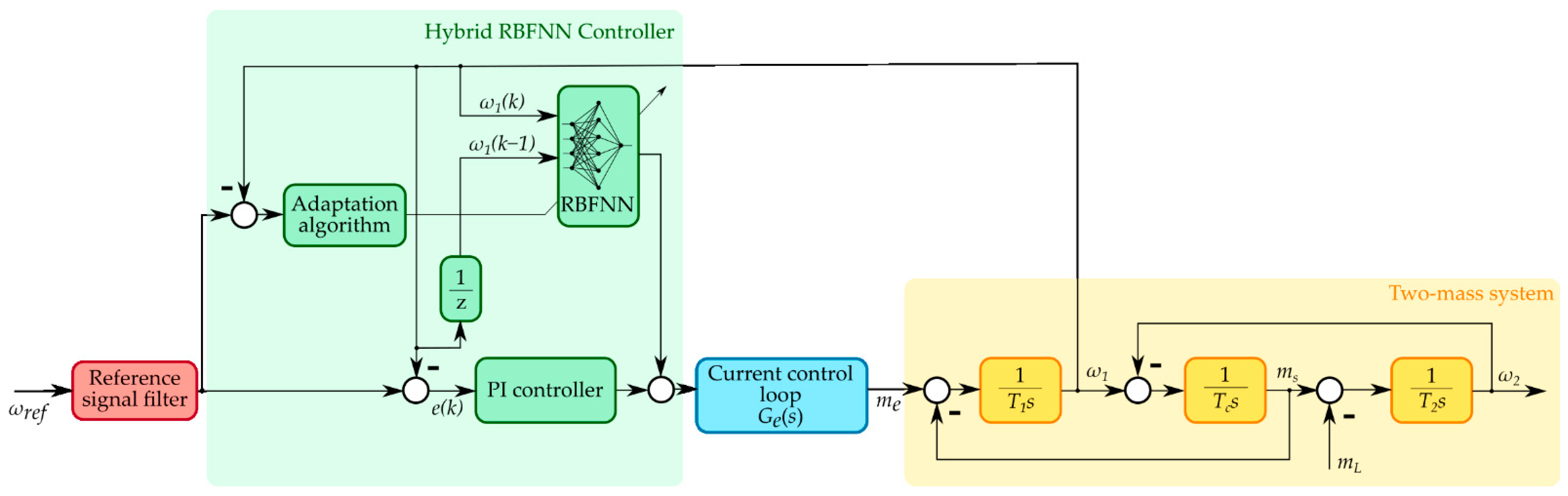
2.1. General Overview and Mathematical Description of the Control Structure

The experimental setup consists of two DC motors connected with a long and elastic shaft. The mechanical part of the considered drive system can be described using the following system of equations (using per unit notation) [41]:

$$\{\begin{array}{c}{\dot{\omega }}_1=\frac{1}{T_1}\left(m_e-m_s\right)\\ {\dot{\omega }}_2=\frac{1}{T_2}\left(m_s-m_L\right)\\ {\dot{m}}_s=\frac{1}{T_c}\left({\omega }_1-{\omega }_2\right)\end{array} ,$$	(1)
	(2)
	(3)

where m_e—electromagnetic torque, m_s—shaft torque, m_L—load torque, ω₁—motor speed, ω₂—load speed, T₁—mechanical time constant of the motor, T₂—mechanical time constant of the load, T_c—mechanical time constant associated with the stiffness of the shaft; the upper dot is used to designate the time derivative.

The proposed control structure is presented in Figure 1. For this research, the values of the time constants were obtained from the drive identification process and used to parametrize the simulation model. The part of the system responsible for the control of the electromagnetic torque m_e can be represented using a transfer function:

$$G_e\left(s\right)=\frac{1}{T_{me}s+1},$$

(4)

where T_me is the time constant of the current control loop. The assumption that T_me > 0, allows representing the drive’s response to the control signal more accurately (with relation to the real object). However, to simplify the following calculations, it is assumed that the transfer function G_e(s) = 1.

Substituting the derivative with the Laplace operator “s”, the system of Equations (1)–(3) can be rewritten as

$$\{\begin{array}{c}{m}_e{=sT}_1{\omega }_1{+m}_s\\ m_s{=sT}_2{\omega }_2{+m}_L\\ {\omega }_1{=sT}_c{m}_s{+\omega }_2\end{array}.$$	(5)
	(6)
	(7)

From here, the following expression describing the electromagnetic torque can be derived

$$m_e{=s}^3{T}_1{T}_2{T}_c{\omega }_2{+s}^2{T}_1{T}_c{m}_L{+sT}_1{\omega }_2{+sT}_2{\omega }_2{+m}_L.$$

(8)

Assuming that the output of the RBFNN is always equal to 0, the electromagnetic torque can also be represented by the following equation:

$$m_e{=G}_R{(\omega }_{ref}-{\omega }_1),$$

(9)

where G_R is a transfer function describing the PI controller defined as

$$G_R=\frac{K_P{s+K}_I}{s}$$

(10)

with K_P standing for the gain of the proportional part of the controller and K_I standing for the gain of the integral part of the controller.

Under the assumption that m_L = 0, the control system can be represented as a transfer function G(s) defined as

$$G\left(s\right)=\frac{{\omega }_2}{{\omega }_{ref}}=\frac{G_R\left(s\right)}{s^3{T}_1{T}_2{T}_c{+s}^2{T}_2{T}_c{G}_R\left(s\right)+s\left(T_1{+T}_2\right){+G}_R\left(s\right)}.$$

(11)

After inserting Equation (10) into (11), the characteristic equation H(s) can be achieved:

$$H\left(s\right){=s}^4{+s}^3\left(\frac{K_P}{T_1}\right){+s}^2\left(\frac{K_I}{T_1}+\frac{1}{T_1{T}_c}+\frac{1}{T_2{T}_c}\right)+s\left(\frac{K_P}{T_1{T}_2{T}_c}\right)+\frac{K_I}{T_1{T}_2{T}_c}$$

(12)

To obtain the values of the controller parameters, the polynomial H(s) must be compared to a reference polynomial of the same order. In this study, the reference polynomial is described as

$$R\left(s\right)=\left(s^2{+2s\xi }_0{\omega }_0{+\omega }_0^2\right)\left(s^2{+2s\xi }_0{\omega }_0{+\omega }_0^2\right),$$

(13)

where ω₀—resonant frequency and ξ₀—damping factor. After the comparison, the following system of equations can be formed:

$$\{\begin{array}{c}\begin{array}{c}{4\xi }_0{\omega }_0=\frac{K_P}{T_1}\\ {\omega }_0^2\left({2+4\xi }_0^2\right)=\frac{K_I}{T_1}+\frac{1}{T_1{T}_c}+\frac{1}{T_2{T}_c}\end{array}\\ \begin{array}{c}{4\xi }_0{\omega }_0^3=\frac{K_P}{T_1{T}_2{T}_c}\\ {\omega }_0^4=\frac{K_I}{T_1{T}_2{T}_c}\end{array}\end{array}$$	(14)
	(15)
	(16)
	(17)

By solving the above-mentioned system of equations, the values of the PI controller parameters can be calculated using the following formulas:

$$K_P=2\sqrt{\frac{T_1}{T_c}}$$

(18)

$$K_I=\frac{T_1}{T_2{T}_c}$$

(19)

Establishing the system’s transfer function G(s) enabled the possibility to extract the pole-zero map of the system, which is presented in Figure 2. The poles are marked with red crosses and the zero is marked with a red circle. Based on the analysis of the map, the damping coefficient ξ is equal to 0.5, while the resonating frequency ω₀ = 64.1 rad/s. The expected overshoot of the system’s step response is estimated at approximately 16.3% of the reference value.

According to the mathematical description presented above, the reason for the oscillations in the analyzed system is the shaft between the motor and the load. The appearing phenomenon is dependent on the parameters of the mechanical part of the drive:

$$\{\begin{array}{c}{T}_1=\frac{J_1{\omega }_n}{m_n}\\ T_2=\frac{J_2{\omega }_n}{m_n}\\ T_c=\frac{m_n}{\theta {\omega }_n}\end{array}$$	(20)
	(21)
	(22)

where J₁—the inertia of the motor, J₂—the inertia of the load, m_n—the nominal torque of the electrical machine, ω_n—the nominal speed of the electrical machine, θ—the stiffness coefficient.

The internal damping factor can be calculated using the formula:

$$\upsilon =\frac{Y{\omega }_n}{m_n}$$

(23)

where Y—the internal damping of the connecting element.

Real objects often contain small natural damping features (for simplification v = 0 was assumed). It should be also noted that in this consideration the analysis is performed using the per-unit values. Then, the resonant (f_r) and anti-resonant (f_ar) frequencies can be determined with the following equations:

$$f_r=\sqrt{\frac{T_1+T_2}{T_1{T}_2{T}_c}}$$

(24)

$$f_{ar}=\sqrt{\frac{1}{T_2{T}_c}}$$

(25)

The parameters defined above are dependent on the correlation between the two-mass system parameters. For the analysis of the time constants and their influence on the oscillations dampening, two transfer functions are determined:

$$G_{\omega 1}\left(s\right)=\frac{{\omega }_1}{m_e}=\frac{s^2{T}_2{T}_c+s\upsilon T_2+1}{s^3{T}_1{T}_2{T}_c+s^2\upsilon T_c\left(T_1+T_2\right)+s\left(T_1+T_2\right)}$$

(26)

$$G_{\omega 2}\left(s\right)=\frac{{\omega }_2}{m_e}=\frac{s^2\upsilon T_2+1}{s^3{T}_1{T}_2{T}_c+s^2\upsilon T_c\left(T_1+T_2\right)+s\left(T_1+T_2\right)}$$

(27)

The Bode plots (Figure 3) show responses of the two systems defined with Equations (26) and (27). The “n” introduced into the plot legend means the nominal values of the parameters. The first is the relation between the input signal—the electromagnetic torque m_e—and the motor speed ω₁. It contains two significant “skips” at the resonant and the anti-resonant frequency, which are visible in Figure 3a,c,e (it is related to the reaction of the additional mass). The second part of the results (Figure 3b,d,f) shows the complete response of the system (Equation (27)). For the nominal values of the time constants (T₁ = 0.203 s, T₂ = 0.203 s, T_c = 0.0012 s), the following frequencies are observed in the transients: f_r = 90.61 Hz and f_ar = 64.07 Hz. These values are different for various conditions of the mechanical part of the drive. Increasing the value of T₁, T₂ and T_c causes a decrease in the resonant frequency. However, in the case of T₁ fluctuation, the values of the anti-resonant frequency do not change for the relation between the motor speed and the electromagnetic torque (Figure 3c). Moreover, the oscillations are dependent on the coefficients of the object. Damping of the plant is lower for lower values of the shaft time constant and higher values of the mechanical time constant of the motor. The changes of T₂ do not introduce the unequivocal behavior of the oscillating system (Figure 3e,f). For transmittance (27) greater value of inertia of the second mass causes better oscillation damping while the increase in the constant T₂ leads to the system excitation if the second mass is not directly controlled (transmittance (26)). The phenomena analyzed above affect the applied speed controller of the two-mass system. It should be also noted that these coefficients can vary under exploitation of the drive. Damping of the torsional vibrations can be difficult for controllers with fixed gains (they are designed for only one operating point). Thus, the application of the parallel combination of the classical PI controller and the RBFNN can lead to a higher precision of control.

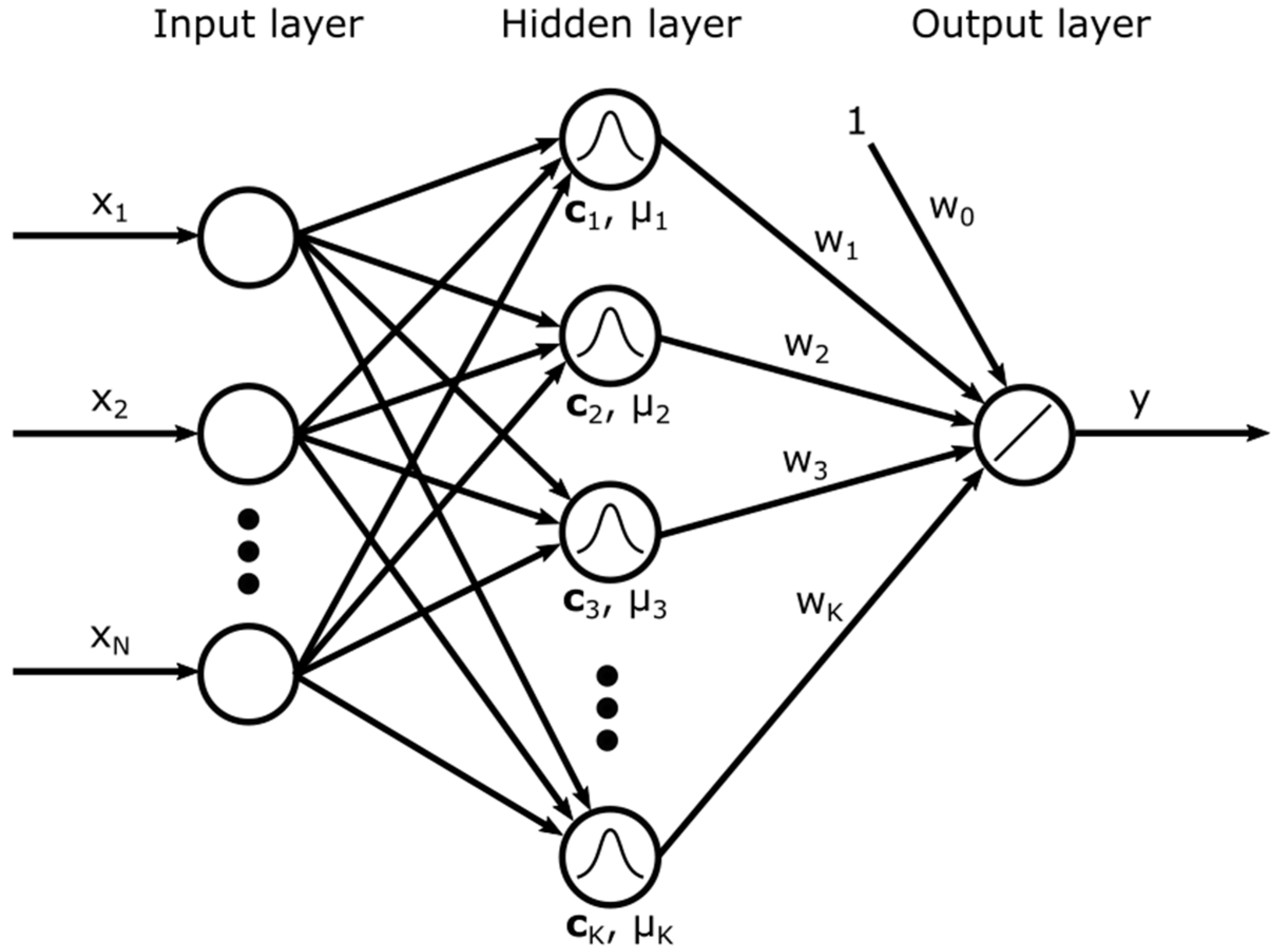
2.2. Radial Basis Function Neural Networks

Radial basis function neural networks are a special case of feed-forward neural networks. A general structure of such a network is presented in Figure 4. Its main distinguishing features are that it always consists of three layers (the input layer, the hidden layer, and the output layer) and that each of the hidden layer’s neurons represents a cluster of the input data space. Global mapping of the data space is accomplished through the superposition of the hidden layer output signals in the output layer neuron [42,43]. The neurons in the hidden layer have radial activation functions that are characterized by their centers C and widths σ. Gaussian functions are often selected for the nodes in the internal layer. The output of a radial neuron in the hidden layer can be described as follows [44]:

$$h_i\left(\mathit{X}\right)=\exp \left(-\frac{{\Vert \mathit{X}-{\mathit{C}}_i\Vert }^2}{{2\sigma }^2}\right),$$

(28)

where X—the input vector, X = [x₁,x₂,x₃,…,x_n]^T, ‖X − C_i‖—Euclidean distance between the input vector and the i-th center, h_i—the output of the i-th hidden neuron.

The output neuron’s activation function is usually linear. With this assumption, the output of the network can be then calculated as a weighted sum of all the hidden layer’s neurons and a bias node:

$$y_{rbf}\left(\mathit{X}\right)={{\displaystyle \sum }}_{i=1}^N{w}_i{h}_i{+w}_0={{\displaystyle \sum }}_{i=1}^N{w}_i\exp \left(-\frac{{\Vert \mathit{X}-{\mathit{C}}_i\Vert }^2}{{2\sigma }_i^2}\right){+w}_0.$$

(29)

In general, the training of the network can be conducted in two steps [45]. First, the values of the widths and centers of the hidden layer activation functions should be determined. Then, the values of the weights and the bias node between the hidden and output layers should be optimized.

For weight optimization, the online approach is selected. The gradient descent method is used for adjusting the values of the weights. The cost function to be minimized is described using the formula presented below [46]:

$$E\left(k\right)=\frac{1}{2}{\left(d\left(k\right)-y_{rbf}\left(k\right)\right)}^2,$$

(30)

where y_rbf—the output of the RBFNN, d—the desired value of the output, and k—the current iteration.

The change of the i-th weight can then be described as a rate of change of the cost function with regard to the i-th weight multiplied by a constant given as

$$\Delta w_i\left(k\right)=\eta \frac{\partial E\left(k\right)}{\partial w_i\left(k\right)},$$

(31)

where η—the learning rate.

Combining Equations (29)–(31), the change of the i-th weight can be rewritten as:

$$\Delta w_i\left(k\right)=-\eta \left(d\left(k\right)-y_{rbf}\left(k\right)\right)h_i\left(k\right).$$

(32)

The new value of the i-th weight can be obtained using the following formula:

$$w_i\left(k+1\right){=w}_i\left(k\right){+\Delta w}_i\left(k\right).$$

(33)

The structure of the neural network used in this work consists of two inputs—the speed of the motor in the k-th and the (k − 1)-th iteration, five radial neurons in the hidden layer, and a single output neuron with a linear activation function. Both the values of the centers C and the widths σ of the hidden layer neurons’ activation functions are selected arbitrarily. The initial values for the weights are generated randomly. The output of the neural network is one of the constituents of the speed controller output signal.

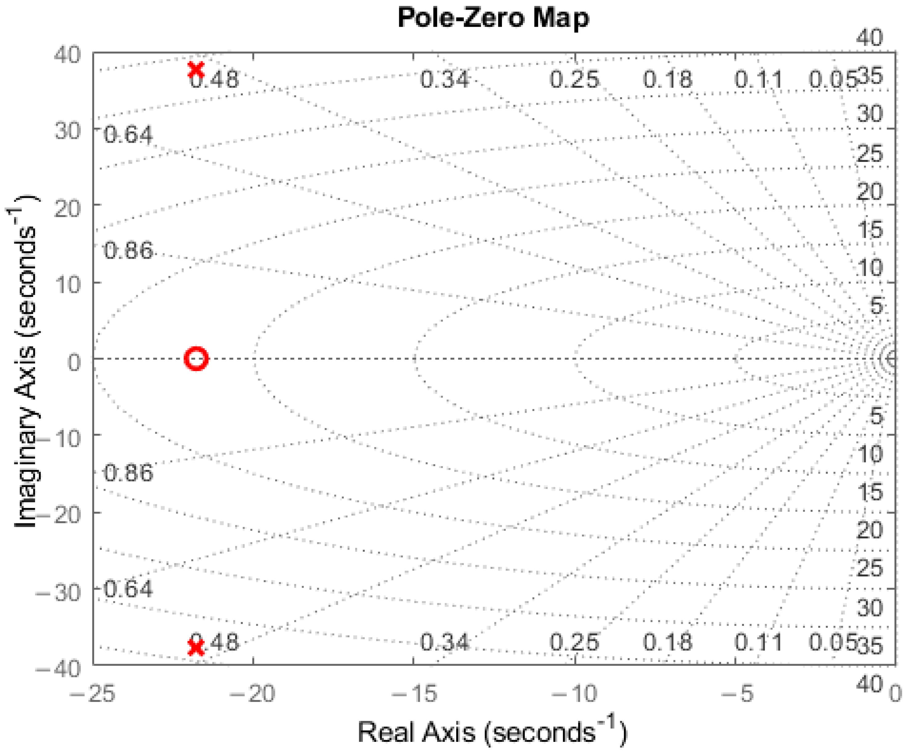
2.3. Stability Analysis

In this study, the purpose of the neural network is to minimize the effect of the difference between the real plant and the identified model of the plant on the estimation of the control signal. Thus, compensation is achieved:

$$\Delta =\hat{f}\left(x\right)-f\left(x\right){=u}_{rbfo}+\epsilon ,$$

(34)

where u_rbfo is the optimal signal of the neural network with the weight matrix W₀ containing the ideal values of the weights, f(x) is a function describing the real plant and $\hat{f}\left(x\right)$ is the identified model of the plant. The obtained training error ε must be relatively low to attain control precision. The upper boundary can be assumed as follows:

$$\epsilon \triangleq \underset{{\mathit{X}}_{rbf}}{\sup }\Vert \widehat{f}\left(x\right)-f\left(x\right)\Vert .$$

(35)

The Lyapunov function, for this analysis, takes the following form

$$L=\frac{1}{2}{\Sigma }^T\mathit{P}\Sigma +\frac{1}{2}tr\left({\tilde{\mathit{W}}}^T\mathsf{\Xi }\tilde{\mathit{W}}\right),$$

(36)

where

$$\Sigma =\left[\begin{array}{c}\int e\\ e\end{array}\right],$$

(37)

e—the error between the reference state of the plant x_ref and the actual state of the plant x, P—a positive definite matrix, Ξ—a nonnegative matrix, tr—a trace of the matrix, and $\tilde{\mathit{W}}$—the difference between the optimal and the actual matrix of the RBFNN’s weights.

If stable work of the control structure is to be achieved, $\dot{\mathit{L}}$ must be non-positive:

$$\dot{\mathit{L}}\le 0 .$$

(38)

Therefore, the following derivative of the Lyapunov function is introduced:

$$\dot{\mathit{L}}=\frac{1}{2}{\dot{\Sigma }}^T\mathit{P}\Sigma +\frac{1}{2}{\Sigma }^T\dot{\mathit{P}}\Sigma +\frac{1}{2}{\Sigma }^T\mathit{P}\dot{\Sigma }+tr\left({\tilde{\mathit{W}}}^T\mathsf{\Xi }\dot{\tilde{\mathit{W}}}\right).$$

(39)

After assuming a positive definite matrix Q according to the Lyapunov equation [47], we can derive:

$$\mathit{Q}=-\left(A^T\mathit{P}+\mathit{P}A\right),$$

(40)

where:

$$A=\left[\begin{array}{cc}0& 1\\ -K_I& -K_P\end{array}\right],$$

(41)

and with matrix B:

$$\mathit{B}=\left[\begin{array}{c}0\\ 1\end{array}\right],$$

(42)

Equation (39) can be transformed into

$$\dot{\mathit{L}}=-\frac{1}{2}{\Sigma }^T\mathit{Q}\Sigma +\mathit{B}\epsilon \mathit{P}\Sigma +tr\left({\tilde{\mathit{W}}}^T\mathsf{\Xi }\dot{\tilde{\mathit{W}}}+\mathit{B}{\tilde{\mathit{W}}}^T\mathsf{\phi }\mathit{P}\Sigma \right).$$

(43)

Furthermore, an adaptation law can be presented as

$$\dot{\widehat{\mathit{W}}}=\frac{1}{\mathsf{\Xi }}\mathit{B}\mathit{\phi }\mathit{P}\Sigma .$$

(44)

Using the information about the derivative of the weight matrix error $\dot{\tilde{\mathit{W}}}$, it can be derived that in (43) the part with the trace of the matrix is equal to 0, hence $\dot{\mathit{L}}$ can be described as

$$\dot{\mathit{L}}=-\frac{1}{2}{\Sigma }^T\mathit{Q}\mathit{P}+\mathit{B}\epsilon \mathit{P}\Sigma .$$

(45)

Assuming λ₁ = −1/2 Σ^T QΣ and λ₂ = BεPΣ, it can be seen that λ₁ is always non-positive. Therefore, the control structure is stable if the training error value is relatively small, considering the boundary presented in Equation (35).

3. Tests of the Hybrid Controller Applied to the Drive with an Elastic Coupling

The testing stage of the work is divided into two parts. First, the simulations are conducted. This stage mainly focuses on finding a set of parameters for the hybrid controller, that would provide both the oscillation damping and adaptive properties. The laboratory experiment results are then presented as confirmation of the superiority of the proposed control strategy over the classical PI controller.

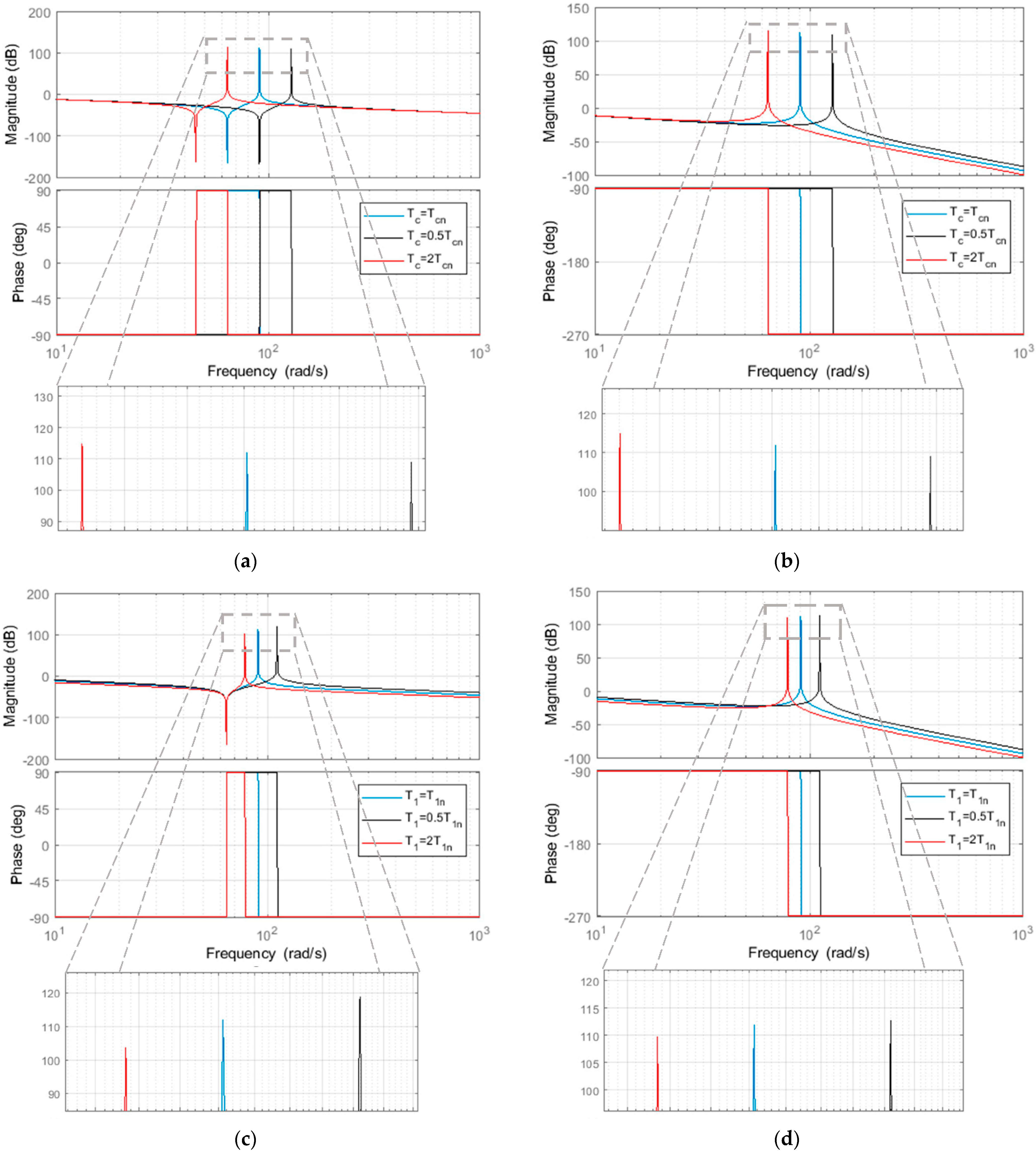
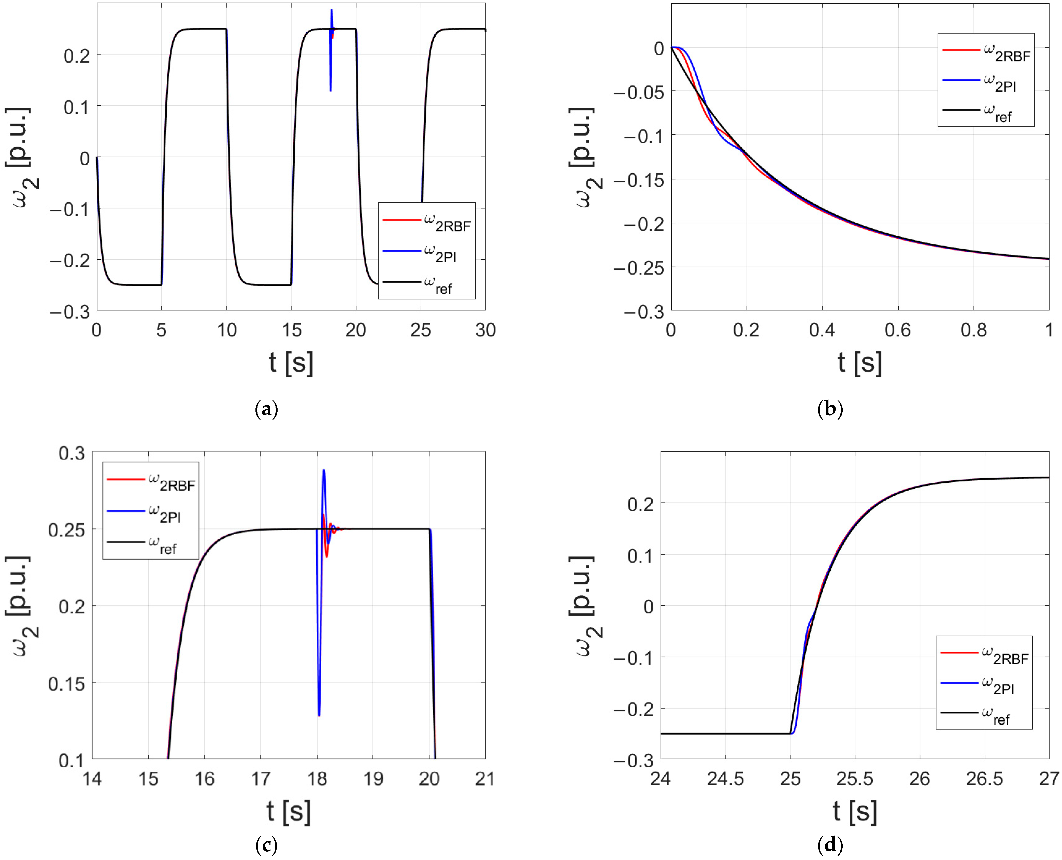
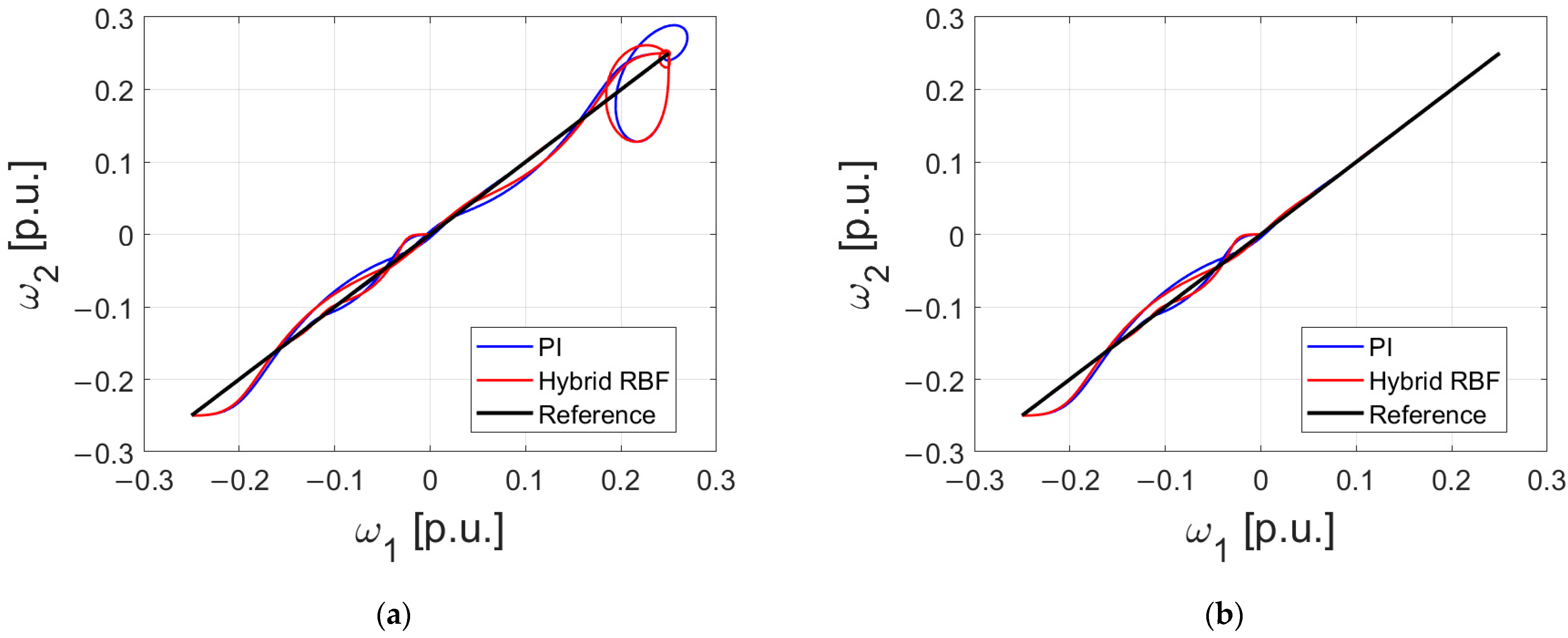
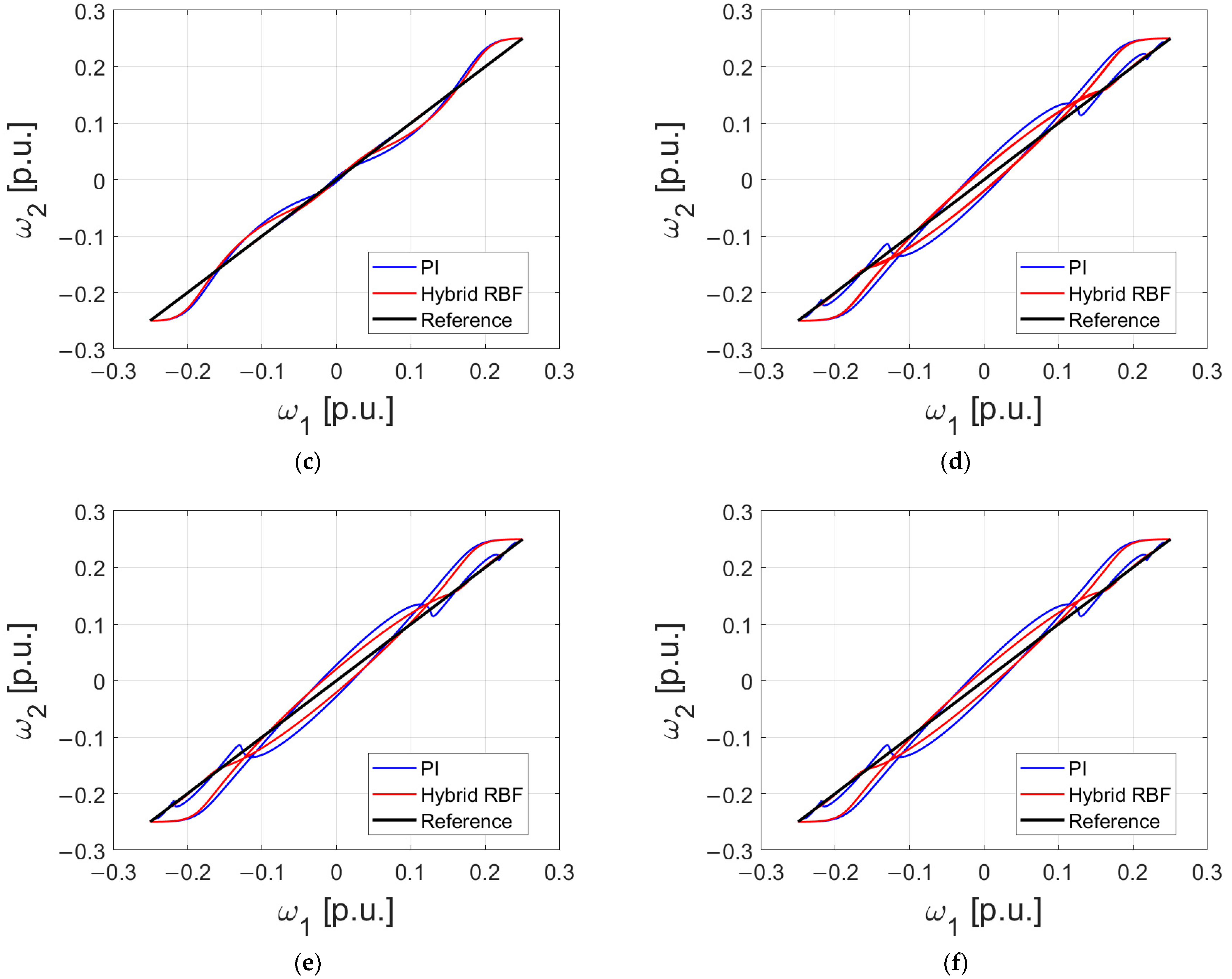
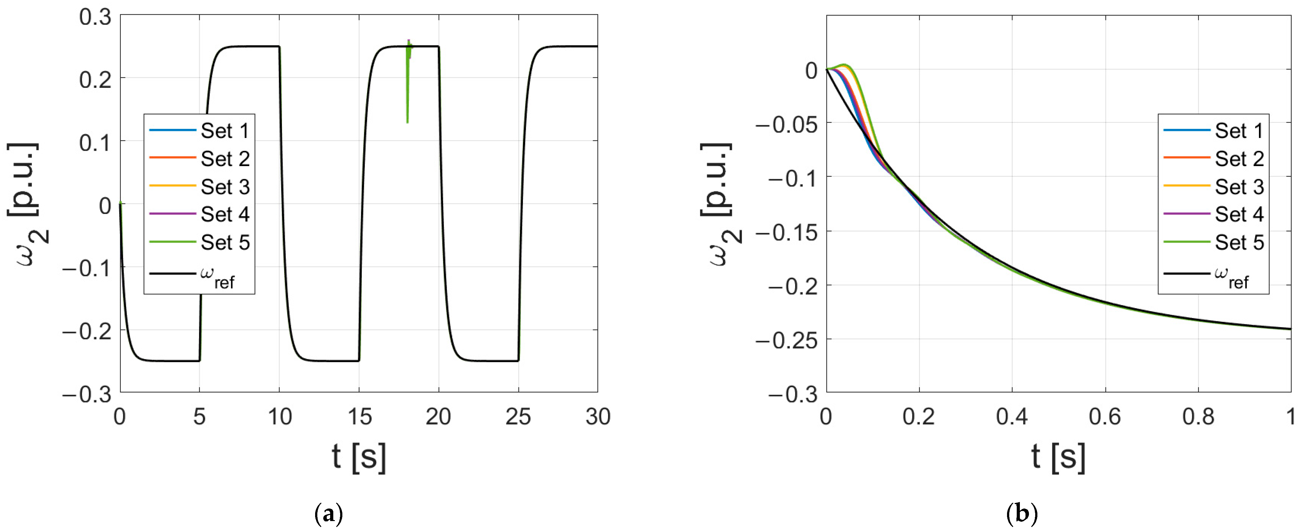
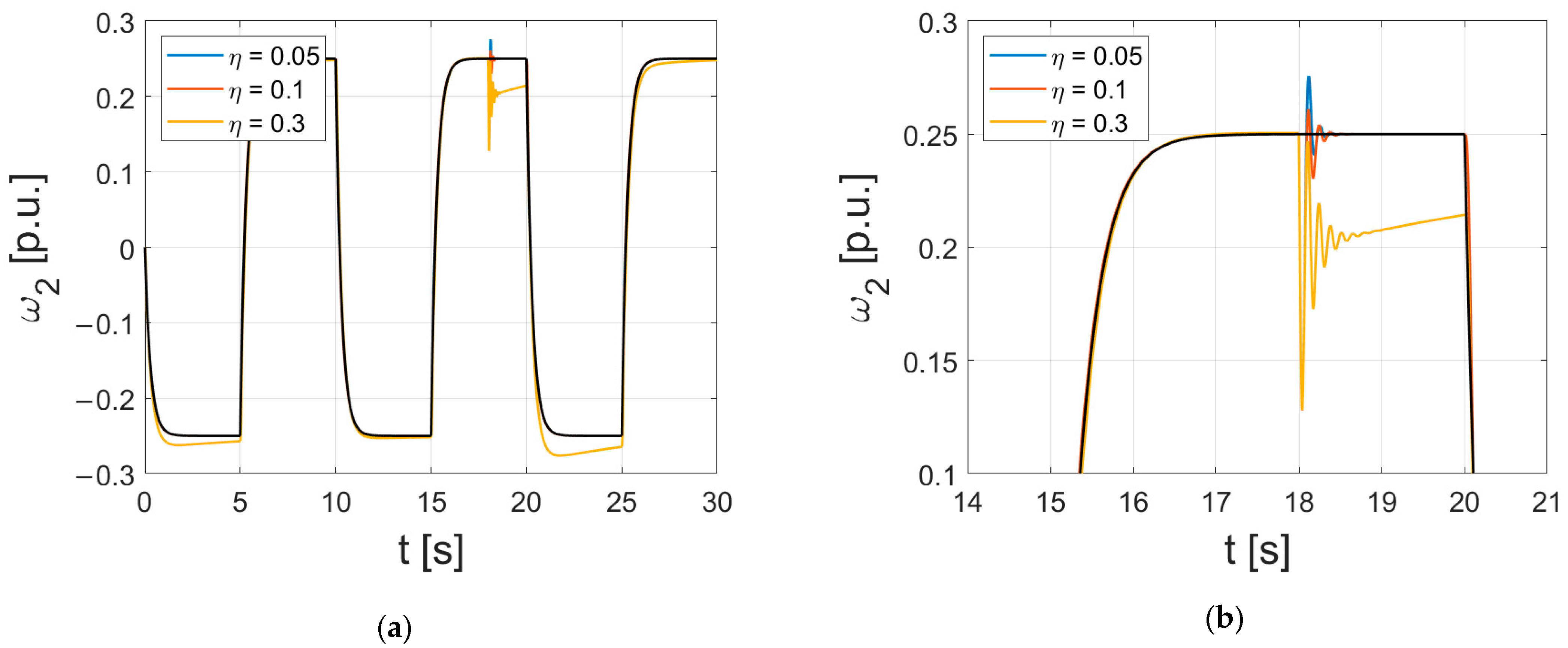
3.1. Simulation Results

The control structure presented in Figure 1 was modeled in the Matlab/Simulink environment and then tested through simulations. The step assumed for numerical calculations was equal to 0.1 ms. As for the reference signal, the periodic square waveform was selected. The recurring occurrence of an input error provides the chance to showcase the adaptive qualities of the proposed control scheme. The weights of the RBFNN were selected randomly at the beginning of the simulation and their updates were then calculated with the learning coefficient η being equal to 0.1. At t_s = 30 s the time constant T₂ is increased four times, thus creating a scenario where the PI controller’s gains are tuned inadequately to the drive’s parameters.

First, the general results of the simulation of the proposed control structure are presented. These tests were performed for the nominal values of the time constants. In Figure 5a, the load speed ω₂ of both the classic PI and the hybrid controller structures are compared to the reference speed value ω_ref. In Figure 5b a closer look at the beginning stage of the system’s operation under normal, unchanged conditions can be observed. The main difference between the algorithms lies in the response to the application of the load, which can be observed in Figure 5c. The overshoot resulting from the sudden load application is lower for the proposed hybrid controller. The work of the system with the load applied can be seen in Figure 5d. Slightly bigger oscillations can be observed for the classical structure at the beginning of the reversion.

Subsequently, the impact of the change in the system’s parameters was verified. The tests were conducted to verify the impact of T₂ increased four times. The results are shown in Figure 6. Even greater improvement can be observed in this scenario—for the proposed hybrid controller the transition between the steady-states is smoother, less oscillating, and has no overshoot.

The tests were also carried out to verify the relationship between the rotational speed of the load with the rotational speed of the motor. The results of the proposed control structure were compared to the results obtained for the classical PI cascade control structure. Linear dependency is expected—it shows that damping of the disturbances from the elastic shaft is achieved and that the system works as a rigid connection. Tests were conducted for two scenarios: the work under normal operating conditions and with the doubled value of T₂. The correlation can be observed in Figure 7a–f. Results of the complete simulation (Figure 7a) include the activation of the load. It is noted as “loops” (close to the point [0.25; 0.25]). Drive starts from 0 [p.u.] to −0.25 [p.u.], the adaptation of the weights in the neural network is the most active (due to the recalculation from the random to the optimal values). It is visible as low oscillations. Then, after the drive reversion, the network works correctly and the difference between the speeds is compensated (the linear part of the transient—Figure 7b). The following part of the simulation shows better results for the hybrid controller (Figure 7c). After the change of T₂, improvements are also observed: both ω₁ and ω₂ overshoots are reduced and the shape of the transition between the steady states is corrected.

The impact of the randomization of the weights and the learning coefficient’s value was also tested. The obtained results are presented in Figure 8 and Figure 9, respectively. Different sets of the initial values of the weights do not alter the general work of the system, which proves that the control structure is indeed stable. Only a slight difference (which is mitigated within 0.5 s) can be observed at the very beginning of the simulation run.

The proper selection of the learning coefficient is a crucial task. As presented in Figure 9, greater values may cause the weight changes to be too dynamic—the response is even more oscillating, and the system is incapable of following the reference value fast enough to converge before the next reversion. Lower values result in a bigger overshoot due to the slower adaptation process.

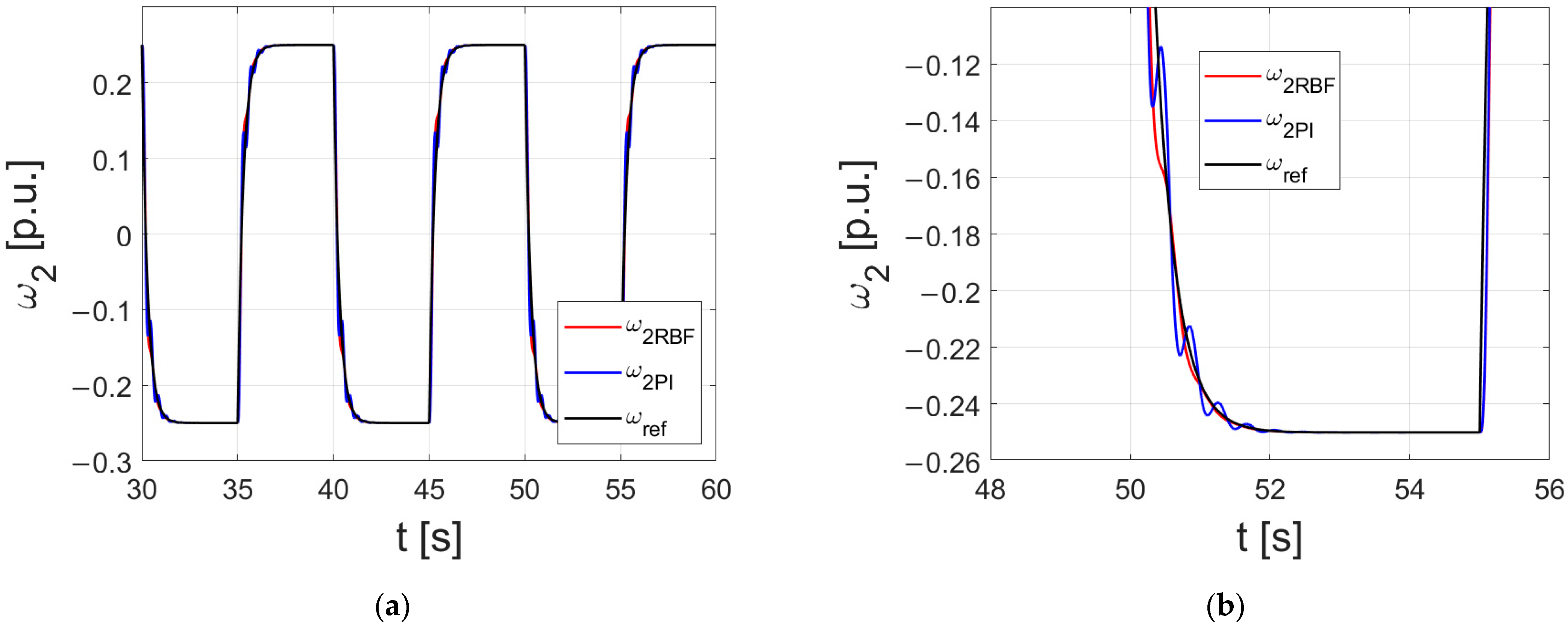
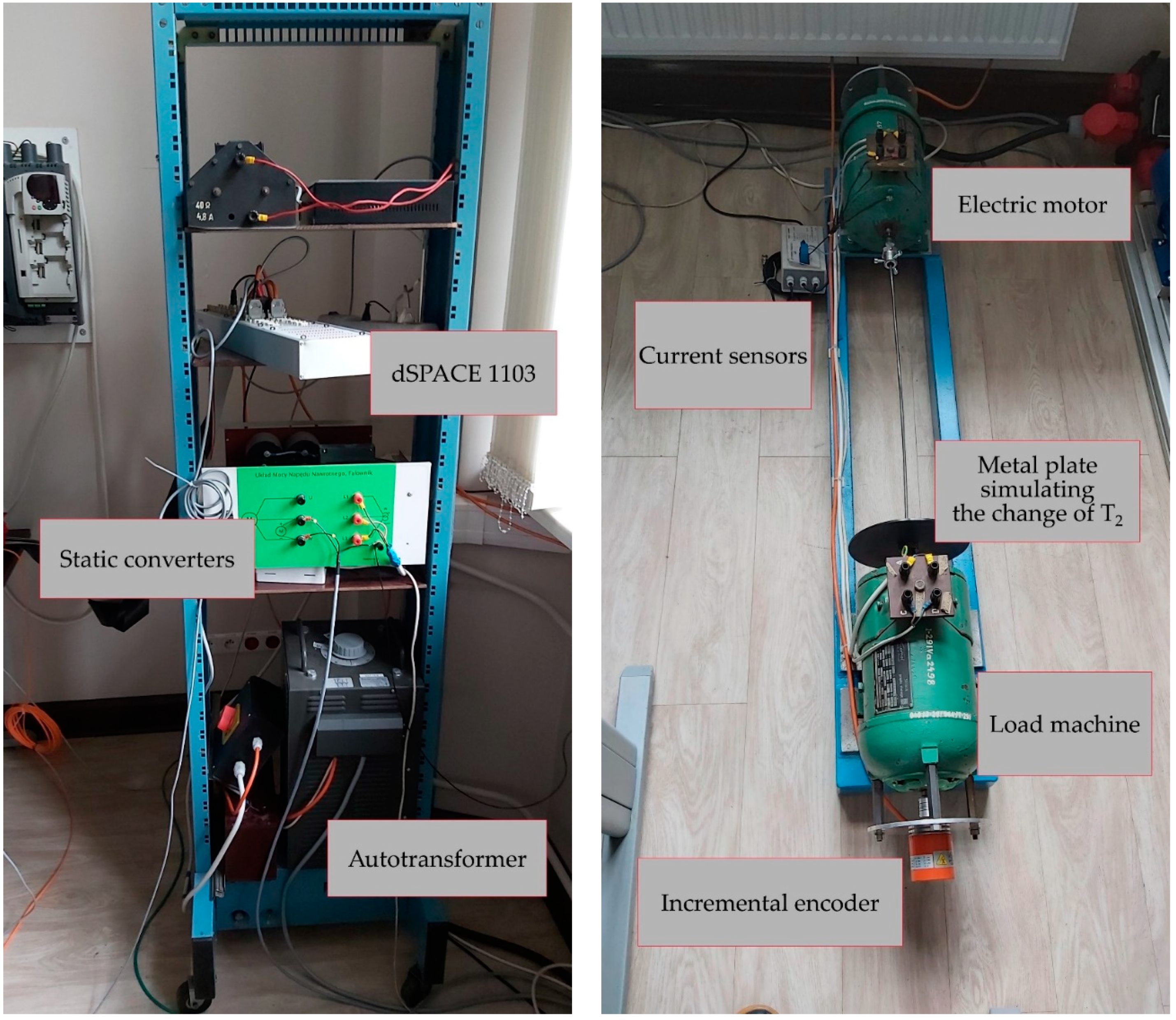
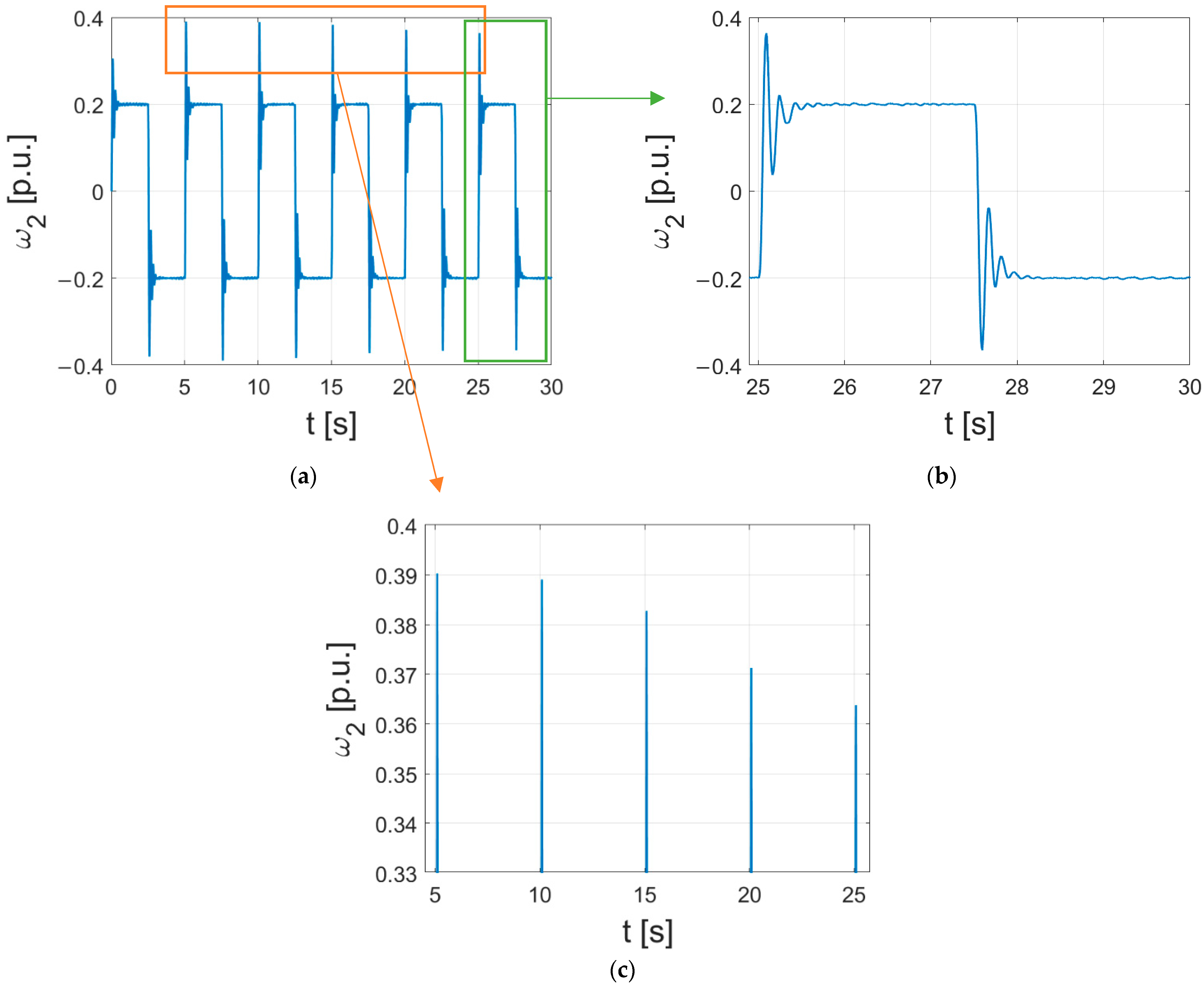
3.2. Experimental Results

The laboratory test bench is comprised of two 500 W DC motors. The nominal ratings of the experimental setup are presented in

Table 1. The parameters of the electrical drive with an elastic connection.

Parameter	Symbol	Value	Unit
Nominal power	PN	500	W
Nominal angular speed	nN	1450	min−1
Motor mechanical time constant	T1	0.203	s
Load mechanical time constant	T2	0.203	s
Shaft mechanical time constant	Tc	0.0026	s

. The machines are connected with a shaft, which is 600 mm long and 7 mm in diameter. The control algorithm is implemented in the dSPACE 1103′s signal processor to designate the PWM signals controlling the operation of the power converters. The machines are powered by their separate static power converters. An incremental encoder (nominal resolution of 36,000 pulses per rotation) is attached to each of the machines to measure the current value of rotational speeds ω₁ and ω₂. The photos of the experimental setup are presented in Figure 10.

The experimental studies were carried out to confirm the results achieved during the simulation tests. The overall work of the system, as well as the impact of the parameters of the RBFNN, were verified.

Verification of the correct operation of the system was conducted in two cases: under normal conditions and with a metal plate mounted on the shaft near the load machine. Attachment of the additional weight allows altering the load machine’s mechanical time constant T₂.

First, the overall work of the hybrid controller structure was investigated. The obtained results can be seen in Figure 11. A zoom-in presenting the convergence of the adaptation algorithm is shown in Figure 11c. The overshoot is lower in value with every reversion; therefore, it can be stated that the adaptation algorithm has a positive impact on the system’s operation. The convergence of the algorithm combined with the stable work of the control structure provides a good basis for further examinations.

The following discussion includes the examination of the impact of weight randomization and the learning coefficient’s value. The results are shown in Figure 12 and Figure 13, respectively. Neither the change in the initial weights nor the different values of the learning coefficient affect the stability of the system—for all the presented cases, the control algorithm manages to follow the reference speed. The one observation worth pointing out is that greater values of the learning coefficient cause the oscillations to be significant; therefore, the value of the learning coefficient must be selected carefully.

The verification of the proper work of the hybrid controller was also carried out for the case, where there was a metal plate attached near the load machine. The additional weight serves the purpose of altering the value of the mechanical time constant of the load machine T₂. The experimental results can be observed in Figure 14. In this case, not only the overshoot but also the oscillations are significantly dampened. This also results in a shorter settling time, making the system much more responsive and safer in operation.

The comparison between the proposed hybrid controller and a classical PI controller was also conducted for this case. The operation of both control structures in these modified conditions is presented in Figure 15. The superiority of the proposed control structure can be clearly observed. Not only the angular speed overshoot is lower, and the speed oscillations are dampened, but also the electromagnetic torque.

4. Discussion

The article proposes an adaptive control structure applied to an oscillating electro- mechanical system. Precisely, a combination of a classic controller (PI type) and a radial basis function neural network (the weights of which were tuned during the operation of the drive) was used for damping of the state variable oscillations. After the theoretical considerations along with the analysis of the simulation results and the experimental transients, the following concluding remarks can be formulated.

➢

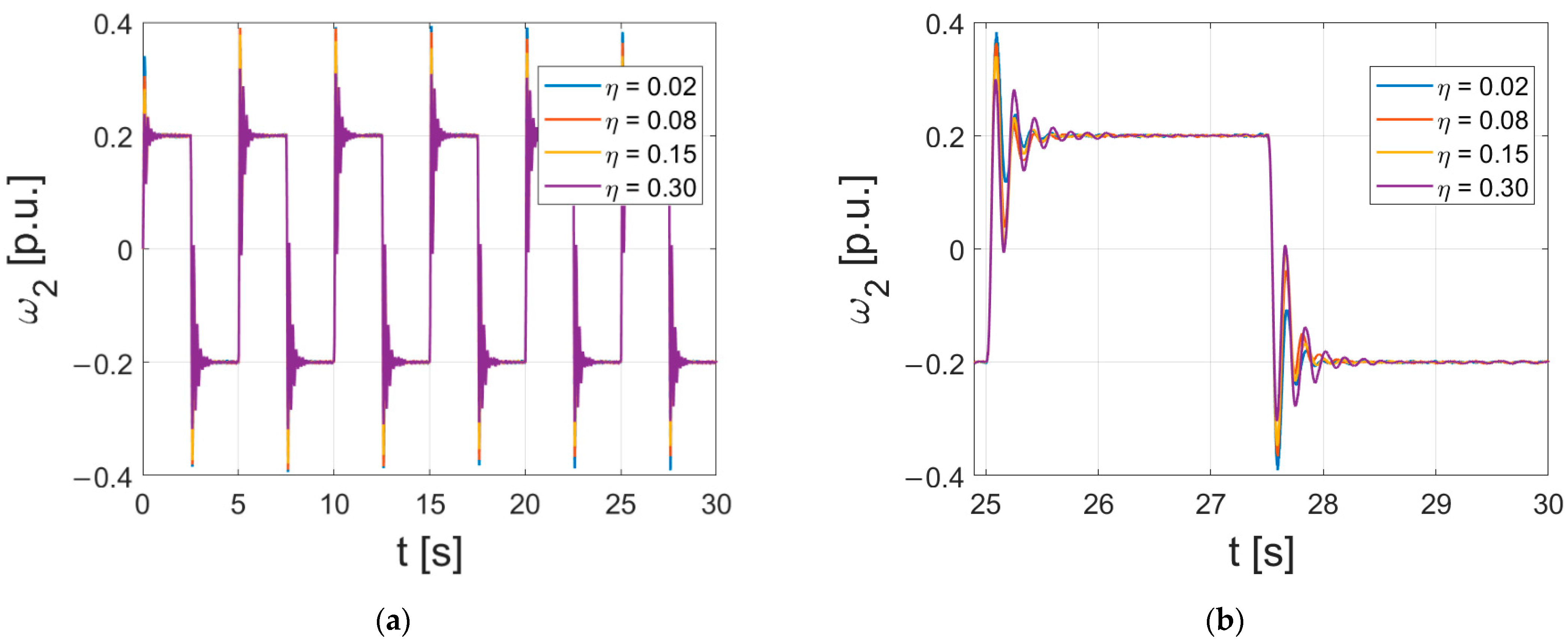
The performance of the drive under the presence of disturbances (changes of the parameters of the two-mass system) obtained for the hybrid controller is distinctively improved—a significant reduction in oscillations was achieved. Moreover, the overshoot resulting from switching the direction of rotation was drastically limited (or even eliminated).

➢

Stable operation of the drive was achieved, values of the weights in the output layer of the RBFNN do not disturb the work of the system (it was confirmed with long-time tests).

➢

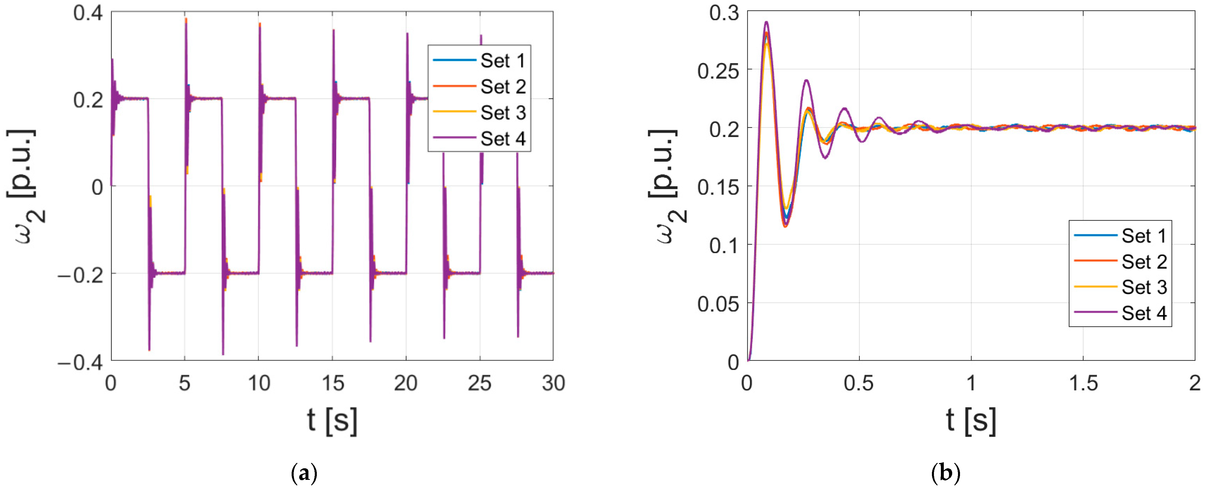
Initial point of the optimization algorithm (the randomization of the network parameters) does not interfere with the correct tracking of the reference speed.

➢

The features observed in simulations were experimentally confirmed (using a rapid prototyping method).

➢

The considered control strategy with a reduced number of used sensors (the feedback loops are based only on the information about the armature current and the speed of the motor) is by far the most difficult to achieve satisfactory results with.

➢

The practical aspect of the proposed control structure deals with a non-extended (compared to the classical solutions) combination of feedback signals. It leads to a reduced number of sensors. Therefore, cost reduction and an increase in system reliability can be achieved.

➢

The additional part of the controller is applied to achieve model-free compensation. It means that the modification of the time constants or other parameters of the object does not affect the correct work of the controller (additional identification of the system does not need to be performed). Reaction to the disturbances is possible due to the recalculation of the network parameters.

The future work, an extension of this project, assumes a comparison with a version of the hybrid controller with additional feedback loops from other state-space variables (with the use of the Kalman filter or the Luenberger observer). Moreover, an FPGA implementation of the algorithm will be conducted.

References

1. Muszynski, R.; Deskur, J. Damping of Torsional Vibrations in High-Dynamic Industrial Drives. IEEE Trans. Ind. Electron. 2010, 57, 544–552. [Google Scholar] [CrossRef]
2. Bosetti, H.; Khan, S. Transient Stability in Oscillating Multi-Machine Systems Using Lyapunov Vectors. IEEE Trans. Power Syst. 2018, 33, 2078–2086. [Google Scholar] [CrossRef]
3. Biagiotti, L.; Melchiorri, C.; Moriello, L. Optimal Trajectories for Vibration Reduction Based on Exponential Filters. IEEE Trans. Control Syst. Technol. 2016, 24, 609–622. [Google Scholar] [CrossRef]
4. Ruf, M. Near time-optimal flexible-joint trajectory planning algorithm for robotic manipulators. In Proceedings of the 2018 IEEE Conference on Control Technology and Applications (CCTA), Copenhagen, Denmark, 21–24 August 2018; pp. 265–272. [Google Scholar] [CrossRef]
5. Magee, D.P.; Book, W.J. Optimal Filtering to Minimize the Elastic Behavior in Serial Link Manipulators. In Proceedings of the American Control Conference, Philadelphia, PA, USA, 26 June 1998. [Google Scholar]
6. Padron, J.; Kawai, Y.; Yokokura, Y.; Ohishi, K.; Miyazaki, T. Stable torsion torque control based on friction-backlash analogy for two-inertia systems with backlash. IEEJ J. Ind. Appl. 2022, 11, 279–290. [Google Scholar] [CrossRef]
7. Chen, Y.; Yang, M.; Sun, Y.; Long, J.; Xu, D.; Blaabjerg, F. A Modified Bi-Quad Filter Tuning Strategy for Mechanical Resonance Suppression in Industrial Servo Drive Systems. IEEE Trans. Power Electron. 2021, 36, 10395–10408. [Google Scholar] [CrossRef]
8. Preitl, S.; Precup, R.E.; Solyom, S.; Kovacs, L. Development of Conventional and Fuzzy Controllers for Output Coupled Drive Systems and Variable Inertia. IFAC Proc. Vol. 2001, 34, 261–269. [Google Scholar] [CrossRef]
9. Hung, J.Y. Control of Industrial Robots that Have Transmission Elasticity. IEEE Trans. Ind. Electron. 1991, 38, 421–427. [Google Scholar] [CrossRef]
10. Ruderman, M.; Iwasaki, M. Sensroless Torsion Control of Elastic-Joint Robots With Hysteresis and Friction. IEEE Trans. Ind. Electron. 2016, 63, 1889–1899. [Google Scholar] [CrossRef]
11. Dhaouadi, R.; Kubo, K.; Tobise, M. Two-Degree-of-Freedom Robust Speed Controller For High Performance Rolling Mill Drives. In Proceedings of the Conference Record of the 1992 IEEE Industry Applications Society Annual Meeting, Houston, TX, USA, 4–9 October 1992; pp. 400–407. [Google Scholar] [CrossRef]
12. Orlowska-Kowalska, T.; Kaminski, M. Application of the OBD method for optimization of neural state variable estimators of the two-mass drive system. Neurocomputing 2009, 72, 3034–3045. [Google Scholar] [CrossRef]
13. Åström, K.; Hägglund, T. PID Controllers: Theory, Design, and Tuning, 2nd ed.; The Instrumentation, Systems, and Automation Society: Research Triangle Park, NC, USA, 1995; pp. 111–116. [Google Scholar]
14. Zhang, G.; Furusho, J. Speed Control of Two-Inertia System by PI/PID Control. IEEE Trans. Ind. Electron. 2000, 47, 603–609. [Google Scholar] [CrossRef]
15. Zhang, G. Comparison of Control Schemes for Two-Inertia System. In Proceedings of the IEEE 1999 International Conference on Power 373 Electronics and Drive Systems. PEDS’99, Hong Kong, China, 27–29 July 1999; pp. 573–578. [Google Scholar] [CrossRef]
16. Saarakkala, S.E.; Hinkkanen, M. State-Space Speed Control of Two-Mass Mechanical Systems: Analytical Tuning and Experimental Evaluation. IEEE Trans. Ind. Appl. 2014, 50, 3428–3437. [Google Scholar] [CrossRef]
17. Pacas, J.M.; John, T.; Eutebach, T. Automatic Identification and Damping of Torsional Vibrations in High-Dynamic-Drives. In Proceedings of the 2000 IEEE International Symposium on Industrial Electronics ISIE’2000, Cholula, Puebla, Mexico, 4–8 December 2000; pp. 201–206. [Google Scholar] [CrossRef]
18. Szabat, K.; Orlowska-Kowalska, T. Vibration Suppression in a Two-Mass Drive System Using PI Speed Controller and Additional Feedbacks-Comparative Study. IEEE Trans. Ind. Electron. 2007, 54, 1193–1206. [Google Scholar] [CrossRef]
19. Derugo, P.; Szabat, K. Damping of Torsional Vibrations of Two-Mass System Using Adaptive Low Computational Cost Fuzzy PID Controller. In Proceedings of the 2015 IEEE 11th International Conference on Power Electronics and Drive Systems, Sydney, Australia, 9–12 June 2015; pp. 1162–1165. [Google Scholar] [CrossRef]
20. Xing, Y.; Wang, X.; Yang, D.; Zhang, Z. Sensorless Control of Permanent Magnet Synchronous Motor Based on Model Reference Adaptive System. In Proceedings of the 2017 10th International Symposium on Computational Intelligence and Design (ISCID), Hangzhou, China, 9–10 December 2017; pp. 20–23. [Google Scholar] [CrossRef]
21. Vazifehdan, M.; Zarchi, H.A.; Khoshhava, M.A. Sensorless Vector Control of Induction Machines via Sliding Mode based Model Reference Adaptive System. In Proceedings of the 2020 28th Iranian Conference on Electrical Engineering (ICEE), Tabriz, Iran, 4–6 August 2020; pp. 1–6. [Google Scholar] [CrossRef]
22. Mohanalakshimi, J.; Suresh, H.N. Sensorless Speed Estimation and Vector Control of an Induction Motor Drive Using Model Reference Adaptive Control. In Proceedings of the 2015 International Conference on Power and Advanced Control Engineering (ICPACE), Bengaluru, India, 12–14 August 2015; pp. 377–382. [Google Scholar] [CrossRef]
23. Nandana, J.; Anas, A.S. An Efficient Speed Control Method for Two Mass Drive Systems using ADALINE. In Proceedings of the 2015 International Conference on Smart Technologies and Management for Computing, Communication, Controls, Energy and Materials (ICSTM), Avadi, India, 6–8 May 2015; pp. 418–423. [Google Scholar] [CrossRef]
24. Lukichev, D.V.; Demidova, G.L.; Brock, S. Fuzzy Adaptive PID Control for Two-Mass Servo-Drive System with Elasticity and Friction. In Proceedings of the 2015 IEEE 2nd International Conference on Cybernetics (CYBCONF), Gdynia, Poland, 24–26 June 2015; pp. 443–448. [Google Scholar] [CrossRef]
25. Li, D.; Zhang, Z.; Liu, P.; Wang, Z.; Zhang, L. Battery Fault Diagnosis for Electric Vehicles Based on Voltage Abnormality by Combining the Long Short-Term Memory Neural Network and the Equivalent Circuit Model. IEEE Trans. Power Electron. 2022, 36, 1303–1315. [Google Scholar] [CrossRef]
26. Wolkiewicz, M.; Kowalski, C.T. Incipient stator fault detector based on neural networks end symmetrical components analysis for induction motor drives. In Proceedings of the 2016 13th Selected Issues of Electrical Engineering and Electronics (WZEE), Rzeszow, Poland, 4–8 May 2016; pp. 1–7. [Google Scholar] [CrossRef]
27. Quintero-Manriquez, E.; Sanchez, E.N.; Felix, R.A. Induction motor torque control via discrete-time neural sliding mode. In Proceedings of the 2016 International Joint Conference on Neural Networks (IJCNN), Vancouver, BC, Canada, 24–29 July 2016; pp. 2756–2761. [Google Scholar] [CrossRef]
28. Azizi, S.; Asemani, M.H.; Vafamand, N.; Mobayen, S.; Fekih, A. Adaptive Neural Network Linear Parameter-Varying Control of Shipboard Direct Current Microgrids. IEEE Access 2022, 10, 75825–75834. [Google Scholar] [CrossRef]
29. Chan, V.M.; Hernández-Vargas, E.A.; Sánchez, E.N. Neural inverse optimal control applied to design therapeutic options for patients with COVID-19. In Proceedings of the 2021 International Joint Conference on Neural Networks (IJCNN), Shenzhen, China, 18–22 July 2021; pp. 1–7. [Google Scholar] [CrossRef]
30. Nebeluk, R.; Lawrynczuk, M. Fast Nonlinear Model Predictive Control Using a Custom Cost-Function: Preliminary Results. In Proceedings of the 2022 30th Mediterranean Conference on Control and Automation (MED), Vouliagmeni, Greece, 28 June–1 July 2022; pp. 13–18. [Google Scholar] [CrossRef]
31. Du, G.; Liang, Y.; Gao, B.; Al Otaibi, S.; Li, D. A Cognitive Joint Angle Compensation System Based on Self-Feedback Fuzzy Neural Network With Incremental Learning. IEEE Trans. Ind. Inform. 2021, 17, 2928–2937. [Google Scholar] [CrossRef]
32. Quintero-Manriquez, E.; Sanchez, E.N.; Harley, R.G.; Li, S.; Felix, R.A. Neural Inverse Optimal Control Implementation for Induction Motors via Rapid Control Prototyping. IEEE Trans. Power Electron. 2019, 34, 5981–5992. [Google Scholar] [CrossRef]
33. Kaminski, M.; Orlowska-Kowalska, T. FPGA Implementation of ADALINE-Based Speed Controller in a Two-Mass System. IEEE Trans. Ind. Inform. 2013, 9, 1301–1311. [Google Scholar] [CrossRef]
34. Li, D.; Liu, P.; Zhang, Z.; Zhang, L.; Deng, J.; Wang, Z.; Dorell, D.G.; Li, W.; Sauer, D.U. Battery Thermal Runaway Fault Prognosis in Electric Vehicles Based on Abnormal Heat Generation and Deep Learning Algorithms. IEEE Trans. Power Electron. 2022, 37, 8513–8525. [Google Scholar] [CrossRef]
35. Roy, S.; Menapace, W.; Oei, S.; Luijten, B.; Fini, E.; Saltori, C.; Huijben, I.; Chennakeshava, N.; Mento, F.; Sentelli, A.; et al. Deep Learning for Classification and Localization of COVID-19 Markers in Point-of-Care Lung Ultrasound. IEEE Trans. Med. Imaging 2020, 39, 2676–2687. [Google Scholar] [CrossRef]
36. Skowron, M.; Orlowska-Kowalska, T.; Kowalski, C.T. Detection of Permanent Magnet Damage of PMSM Drive Based on Direct Analysis of the Stator Phase Currents Using Convolutional Neural Network. IEEE Trans. Ind. Electron. 2022, 69, 13665–13675. [Google Scholar] [CrossRef]
37. Niu, F.; Tian, L.; Li, Y.Y.R.; Norman, T.L. Studies on flow instability of helical tube steam generator with Nyquist criterion. Nucl. Eng. Des. 2014, 266, 63–69. [Google Scholar] [CrossRef]
38. El-Marhomy, A.A.; Abdel-Sattar, N.E. Stability analysis of rotor-bearing systems via Routh-Hurwitz criterion. Appl. Energy 2004, 77, 287–308. [Google Scholar] [CrossRef]
39. Stanisławski, R. Modified Mikhailov stability criterion for continuous-time noncommensurate fractional-order systems. J. Frankl. Inst. 2022, 359, 1677–1688. [Google Scholar] [CrossRef]
40. Nguyen, P.T.H.; Stüdli, S.; Braslavsky, J.H.; Middleton, R.H. Lyapunov stability of grid-connected wind turbines with permanent magnet synchronous generator. Eur. J. Control 2022, 65, 100615. [Google Scholar] [CrossRef]
41. Hara, K.; Hashimoto, S.; Funato, H.; Kamiyama, K. Robust comparison between state feedback-based speed control systems with and without state observers in resonant motor drives. Proc. Second Int. Conf. Power Electron. Drive Syst. 1997, 1, 371–376. [Google Scholar] [CrossRef]
42. Meng, X.; Rozycki, P.; Qiao, J.; Wilamowski, B.M. Nonlinear system modeling using RBF Networks for industrial application. IEEE Trans. Industr. Inform. 2018, 14, 931–940. [Google Scholar] [CrossRef]
43. Zhang, P.; Zhou, X.; Pelliccione, P.; Leung, H. RBF-MLMR: A Multi-Label Metamorphic Relation Prediction Approach Using RBF Neural Network. IEEE Access 2017, 5, 21791–21805. [Google Scholar] [CrossRef]
44. Liu, Z.; Guo, Y.; Gao, M.; Zhao, X.; Zhang, Y. Fuzzy Neural Network Blind Equalization Algorithm Based on Radial Basis Function. In Proceedings of the 2009 International Conference on Intelligent Human-Machine Systems and Cybernetics, Hangzhou, China, 26–27 August 2009; pp. 280–283. [Google Scholar] [CrossRef]
45. Bose, B.K. Modern Power Electronics and AC Drives; Prentice Hall PTR: Upper Saddle River, NJ, USA, 2002; pp. 625–658. [Google Scholar]
46. Wu, W.; Zhong, S.; Zhou, G. A study on PID intelligent optimization based on radial basis function neural networks. In Proceedings of the 2013 3rd International Conference on Consumer Electronics, Communications and Networks, Xianning, China, 20–22 November 2013; pp. 57–60. [Google Scholar] [CrossRef]
47. Simoncini, V. Computational Methods for Linear Matrix Equations. SIAM Rev. 2016, 58, 377–441. [Google Scholar] [CrossRef] [Green Version]
Figure 1. The block diagram of the proposed control structure with the hybrid controller.
Energies 15 06265 g001
Figure 2. The pole–zero map of the analyzed control structure.
Energies 15 06265 g002
Figure 3. The frequency characteristics of the oscillating system: (a) response of the system described with Equation (26) to the changes in Tc; (b) response of the system described with Equation (27) to the changes in Tc; (c) response of the system described with Equation (26) to the changes in T1; (d) response of the system described with Equation (27) to the changes in T1; (e) response of the system described with Equation (26) to the changes in T2; (f) response of the system described with Equation (27) to the changes in T2.
Energies 15 06265 g003aEnergies 15 06265 g003b
Figure 4. A general structure of an RBFNN.
Energies 15 06265 g004
Figure 5. Simulation results—the hybrid controller structure testing: (a) a general overview of the simulation run; (b) a zoom-in showing the initial stage of the simulation; (c) a zoom-in showing the work of the controller when the load is switched on; (d) a zoom-in showing the operation of the drive with the nominal load switched on.
Energies 15 06265 g005
Figure 6. Simulation results—the impact of the system’s parameter change: (a) general overview of the simulation run; (b) a zoom-in showing the work of the controller under different operating conditions.
Energies 15 06265 g006
Figure 7. Simulation results: the correlation between the rotational speeds of the load and the motor: before the change of T2: (a) the whole duration of the simulation; (b) time between 0–10 s; (c) time between 20–30 s; with the increased value of T2: (d) the whole duration of the simulation; (e) time between 0–10 s; (f) time between 20–30 s.
Energies 15 06265 g007aEnergies 15 06265 g007b
Figure 8. The impact of the change of the initial parameters of the RBF neural network: (a) the overview of the simulation run; (b) a zoom-in presenting the initial stage of the simulation.
Energies 15 06265 g008
Figure 9. The impact of the change of the learning coefficient: (a) the overview of the simulation run; (b) a zoom-in presenting the final stage of the simulation.
Energies 15 06265 g009
Figure 10. The experimental set-up: left—power electronic devices, right—electrical machines.
Energies 15 06265 g010
Figure 11. The work of the controller under nominal conditions: (a) the general overview of the experimental run; (b) a zoom-in presenting the final reversions of the experimental run; (c) a zoom-in presenting the highest value of the load angular speed after every reversion.
Energies 15 06265 g011
Figure 12. The impact of the initial values of the RBFNN’s weights: (a) a general overview of the experimental run; (b) a zoom-in at the initial stage of the experimental run.
Energies 15 06265 g012
Figure 13. The impact of a different value of the learning coefficient: (a) a general overview of the experimental run; (b) a zoom-in at the final reversions of the experimental run.
Energies 15 06265 g013
Figure 14. The work of the controller under the altered conditions—an additional plate mounted on the side of the load machine: (a) the general overview of the experimental run; (b) a zoom-in presenting the final reversions of the experimental run; (c) a zoom-in presenting the highest value of the load angular speed after every reversion.
Energies 15 06265 g014
Figure 15. The comparison between the PI controller and the proposed hybrid controller—experimental results: (a) The angular speed of the load—a general overview of the experimental run; (b) a zoom-in at the final reversion of the experimental run; (c) the electromagnetic torque—a general overview of the experimental run; (d) a zoom-in at the torque during the final reversions of the experimental run.
Energies 15 06265 g015