Abstract
The aims of this study were to determine the concentrations and elemental composition of PM10 in the village of Kotórz Mały (Poland), to analyse their seasonal variability, to determine the sources of pollutant emissions and to compare the consistency of the results obtained using different methods. Sampling and weather condition measurements were carried out in the winter (January–February) and spring (April) of 2019. Two combinations of different techniques were used to examine PM10 concentrations and their chemical composition: gravimetric method + atomic absorption spectrometry (GM+AAS) and continuous particle monitor + energy dispersive X-ray fluorescence (CPM+EDXRF). In winter, the average concentrations of PM10 measured by the GM and CPM were similar (GM 44.3 µg/m3; CPM 34.0 µg/m3), while in spring they were clearly different (GM 49.5 µg/m3; CPM 29.8 µg/m3). Both AAS and EDXRF proved that in both seasons, Ca, K and Fe had the highest shares in the PM10 mass. In the case of the lowest shares, the indications of the two methods were slightly different. Factor analysis indicated that air quality in the receptor was determined by soil erosion, coal and burning biomass, and the combustion of fuels in car engines; in the spring, air quality was also affected by gardening activities.
1. Introduction
Particulate matter (PM) released from primary sources or generated and transformed in the atmosphere by reactions can be toxic and may contribute to adverse environmental effects [1,2]. It is well recognised that the presence of above-normal amounts of aerosol in the air is associated with morbidity and mortality as well as annoyance and psychological stress [3,4]. The current research looked at specific locations, seasonal trends, dust properties and relevant control factors [5,6,7,8,9,10,11]. Most research is conducted in highly urbanised areas, mainly cities and agglomerations; the amount of air quality recognition work in rural settlement areas is much less [12].
Particulate matter is a mixture of solid and liquid particles, suspended in the air, originating from both natural and anthropogenic sources [13,14]. The sources of PM in the atmosphere which are then enriched with toxic elements or compounds have been widely investigated in many works, including Rodríguez et al. [15], Majewski et al. [16], Rogula-Kozłowska et al. [17] and Mach et al. [18]. Over the last decade, the number of papers reporting results of studies conducted in the areas of compact rural buildings and small villages has increased. In several papers [19,20,21,22,23,24,25] it was remarked that, in the cold season, the principal source of PM emission is associated with the combustion of conventional fuels in domestic heating systems. Concentrations of aerosol particles within local air sheds are affected also by meteorological parameters [19]. An occasional increase in rural aerosol concentrations was mostly attributed to the transportation of particles from polluted urban or industrial areas and remote natural sources [18,26].
Many methods are used in aerosol testing, including direct measurements, indirect measurements or mathematical modelling [18]. For the study of the mass concentration of particulate matter and its constituents, the reference methods should be the gravimetric method (GM) followed by an analysis by atomic absorption spectrometry (AAS), while other methods may be used if their equivalence to the reference method has been demonstrated [27].
In addition to the AAS technique (and the equivalent ICP-MS technique (Inductively Coupled Plasma Mass Spectrometry)), non-destructive techniques are applicable and are generally referred to as X-ray fluorescence (XRF) [28,29,30,31,32]. The detailed characterisation and application of AAS and XRF were presented in a paper by Galvão et al. [33]. There are many works which confirm the usefulness of XRF as an effective technique to determine the elements in various research materials, for example, soil, mollusc tissues and fish tissues [4,34,35,36]. In addition, authors often focus their attention on studies which compare XRF indications with AAS. Comparative XRF and AAS studies of the same samples (first using non-destructive techniques and then those that require mineralisation of the test material) are usually carried out under laboratory conditions, including an analysis of the Pb content in the same dust samples [37,38], the measurement of metals in ash following the combustion of petroleum oil [39], the detection of metal content in soils [34,36] and a determination of the elements in the previously mentioned animal tissues [4,35]. The results of Bizo et al. [34] clearly showed that there were no statistically significant differences in the elemental concentrations determined by AAS and XRF, noting that AAS had a lower limit of detection (LOD) and limit of quantification (LOQ). Gerboles et al. [40] has also presented interesting research. The authors described the results of inter-laboratory measurements on five samples of identical composition. The measurements used for comparison were graphite furnace atomic absorption spectrometry (GF-AAS), inductively coupled plasma with mass spectrometry (ICP-MS), energy dispersive X-ray fluorescence (EDXRF) and inductively coupled plasma-atomic emission spectrometry (ICP-AES). The results of this research indicated significant agreement between EDXRF and the other techniques. The results of inter-laboratory comparative studies using XRF, ICP-MS and PIXE (particle-induced X-ray emission) to measure elemental loads of Al, K, Ca, Ti, V, Cu, Sr, Fe, Zn and Pb, among others, in PM10 samples were also presented [41]. With the exception of Fe and Zn, the authors showed consistency of results (also between laboratories). Gupta et al. [42] also used AAS and XRF to carry out a comparative study of the metal concentrations of Zn, Ca, Fe, K, Mn, Ni, Pb, Al, Na and Cr in PM2.5 retained on quartz filters. The authors obtained a high correlation coefficient for Al, K and Na.
Portable, fully automatic XRF analysers are also increasingly used in field studies [43,44]. The previously mentioned authors point to the functionality of these instruments, the important compatibility with reference or reference-equivalent methodologies and the possibility to carry out in situ measurements, even for short periods of time. However, it seems that there is still a need to improve knowledge on non-destructive techniques, despite the considerable amount of research work dedicated to their verification that has been carried out with various environmental components. The need for such studies is particularly apparent with regard to the determination of air quality in terms of dust and trace elements present in dust, especially in areas that are hardly monitored. Such areas include dense rural development where, for example, significant anthropogenic emissions take place in the cold season and thus significant local degradation of aero-sanitary parameters occurs. So far, only a few measurement campaigns of particulate matter PM in rural areas have been carried out in Poland [18,19,45,46,47,48]. At the same time, automatic on-line XRF measurement was used only once in a study by Mach et al. [18].
This paper presents and analyses data on PM10 concentrations and their chemical composition. The data were obtained in two measurement campaigns carried out in the winter and spring. The concentration and elemental composition of PM10 were determined using two methods (techniques), that is, GM+AAS and CPM+EDXRF. In addition to checking the air quality in the rural area, the main aim of the study was to compare the aforementioned methods in terms of the possible compatibility of the results. In addition, potential differences in air quality over the two seasons were checked and an attempt to determine the contribution of individual emission sources was made.
The scope, type, place, apparatus and conditions of observation enabled the verification of the following hypotheses:
- Concentration levels of PM10 are identical regardless of the method of sampling and analysis;
- Concentration levels of PM10-bound elements are identical regardless of the method of analysis; and
- Concentration levels of PM10 and PM10-bound elements are identical regardless of the season (winter-spring relation).
2. Materials and Methods
2.1. Observation Site Description
2.1.1. Characteristic of the Village—Location and Sources of Air Pollution
The study was conducted in the village of Kotórz Mały, Opole Voievodeship, Poland (50°73′66.02″ N; 18°05′06.80″ E, 162 m.a.s.l.). Kotórz Mały is a small settlement (with a population of approx. 1100). The location of the sampling point is shown in Figure 1. There are more than 300 buildings within the village, of which 295 are permanently inhabited. The village is characterised by compact development, consisting mainly of storey buildings, and within its boundaries, new buildings (located mainly in the western part) and old buildings (in the eastern part) can be distinguished. The houses are heated individually. A railroad and a district road pass through the village. In close proximity (<10 km), there are two national roads, DK45 and DK46, with a traffic density of approx. 8000 and 9500 vehicles per day, respectively [18]. The village has an agricultural character, although several businesses prosper within its borders, including two carpenter’s shops, two locksmith’s shops, two car painting shops and three motor vehicle workshops. All of these plants are equipped with highly efficient dedusting equipment. There are several significant emitters associated with the cement, food, mining and metals industries in the region where the village is located. Emitters from plants located in the voivodeship’s capital of Opole, which is also the largest city in the region (with 122,000 inhabitants), are also significant. Opole is located 15 km southwest of the village.
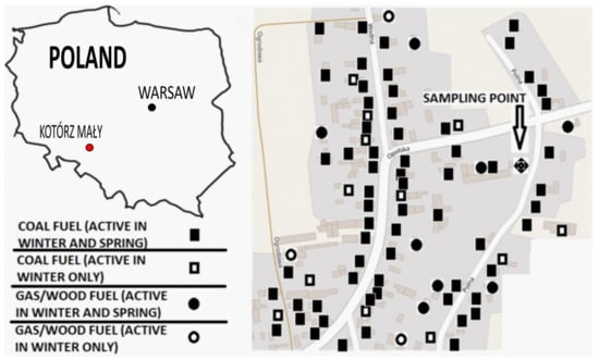
Figure 1.
Location of sampling point with arrangement of point emission sources within a radius of 300 m from the sampling point (without a Renewable Energy Systems-RES; n = 11).
During the warm season, the main source of tropospheric organic and inorganic matter is connected with natural emissions from surrounding areas and anthropogenic emissions from agriculture, traffic, hard coal, wood, biomass, waste and garbage burning in small-scale installations, for example, domestic stoves and local boiler houses [18]. During the cold season, the main local source of air pollution is associated with domestic heating [19].
2.1.2. Characteristics of the Village—Emitters and Fuel Consumption
The sampling point was situated in the dense building area and close to the district road in the old part of the village. As previously mentioned, the study area was characterised by storey rural houses, which predominantly used obsolete individual heating systems (IHS). Coal was mainly used throughout Kotórz Mały in a proportionate share equal to 81% (Table 1). All IHS are usually used during the cold season (form October until April). In the summer, local peoples also use IHS for hot water supply and food preparation, but the number of IHS in use is significantly lower. In the neighbourhood of the sampling point during the measurement campaigns, 86 individual point emitters (IPE) from 97 IHS were active in the winter and 71 in the spring. The location of IPE is shown in Figure 1. The exact number of specific emission sources was determined based on the results of surveys conducted among the residents. The activity of emission sources was indicated on the basis of individual responses of IHS owners and the authors’ own observations. The activity of emitters was periodic and dependent on the needs of users. The average daily time of IPE activity was 17 h in the winter and 14 h in the spring.

Table 1.
Characteristics of Individual Point Emitters (IPE) related to the individual hot water supply and energy for cooking.
A large number of old stoves were in use. More than 80% of heating systems were connected with the burning of fossil fuels or wood. Only 11 items were emission free. Comparing winter and spring fuel consumption, no significant differences were observed related to a single day (Table 2). The large differences in fuel consumption between the winter and spring were related to the different periods of sampling. The relatively high fuel consumption also corresponds to inefficient stoves and the low energy efficiency of the buildings themselves. Of course, the quantity of burned fuel and the relatively long daily use times of fuel source exploitation seems to have influenced local air quality.
Table 2.
Average fuel consumption (Mg) in the single village households during periods of sampling.
Apart from that and agricultural activity typical for rural areas, the local sources of anthropogenic emission were smaller economic activities with services in the fields of woodwork (2 items), vehicle mechanics (2 items) and metal surface varnishing (2 items). These activities were located less than 1 km from the sampling point.
2.2. Sampling and Analysis
The measuring point was equipped with two instruments which realised two different methods of PM10 data collection. First, a reference gravimetric method (GM) with LVS aspirator was used. Samples were collected at 24 h intervals. Second, PM10 mass concentration was measured hourly with an online continuous particle monitor (CPM) which applies reel-to-reel filter tape sampling with beta ray attenuation analysis to determine the total PM10 mass. Both methods were applied at the same time, that is, for 49 consecutive days during the winter period (January–February 2019) and 15 consecutive days during the spring period (April 2019). Because of the need to meet technical conditions, apparatuses were located at a distance of 18 m from each other, with PM10 sampling heads all at the same height above the ground (2.4 m).
2.2.1. PM10 Mass Concentration
In the case of the reference gravimetric method, the mass concentration of PM10 was determined in accordance with the European Standard [49]. The aspiration of the PM10 from the air was provided using low-volume automatic dust sampler Atmoservice PNS-15 aspirator (produced in Poland under the licence for the low-volume sampler LVS 3.1, Comde-Derenda GmbH, Stahnsdorf, Germany). The airflow rate passed filters was 2.3 m3/h. The PM separator applied Whatman QMA quartz air filters with a diameter of 47 mm. Prior to and after aspiration, the filters were seasoned for a minimum 24 h under conditions of constant temperature and humidity and, subsequently, their weight was determined using a differential scale RADWAG XA 52/2X ® (Radwag Balances and Scales, Radom, Poland). The expanded concentration measurement uncertainty, which was calculated on the basis of the guidebook [50], did not exceed 15.2%.
The PX-375 monitor CPM+EDXRF (PX-375 Horiba, Osaka, Japan) was applied for CPM assessment. A two-layer nonwoven Polytetrafluoroethylene (PTFE) fabric filter was used as a filter tape during PM10 collection. The air samples acquisition was achieved by a flow rate equal to 1.002 m3/h. The beta ray attenuation analysis was conducted every 60 min, assessing the exact mass quantity which was based on a rule that absorbed radiation is exponentially dependent only on the mass of filtered material [51]. At the beginning, beta radiation was emitted at an empty filter which gave enough time for sample acquisition and for adsorption of particles on the filter tape. Taking into account the difference between these two measurements, the collected PM10 was given as a result, and then the filter tape was moved to allow for the new measurement. The conditions of the analysis were as follows: 500 s at 15 kV or 50 kV voltage (depending on the element). Samples were collected continuously. For further data comparison, the average daily mass concentration was adopted.
2.2.2. Elements
All samples obtained by GM were analysed by AAS in the laboratory. A microwave oven was used (Start D, Millestone) to digest the quartz filters in Teflon vessels containing a mixture of 8 mL of nitric acid (65%, Merck, Darmstadt, Germany) and 2 mL of hydrogen peroxide (30%, Avantor, Gliwice, Poland). The temperature programme for sample digestion was: 20 min of linearly increasing temperature between ambient and 220 °C, 25 min of constant temperature (220 °C) and 20 min of cooling with 1000 W of power. As suggested by Gerboles et al. [40], this process was performed twice to ensure full digestion of all the dust samples. The mass concentration of metals (Cu, Zn, Cr, Ni, Fe, Mn, K and Ca) was determined by the AAS method, whereas Pb was determined by the GF-AAS method using the Solaar 6M spectrometer (Waltham, MA, USA). The samples after digestion were filtered through a cellulose filter into 25 mL graduated flasks. For high concentrations of metals, the samples were diluted.
Certified material (ERM-CZ120) was prepared and analysed as samples, in triplicate. The recovery (%) from the ERM analysis and LOQ and LOD are presented in Table 3.
Table 3.
Results of the analysis of certified material ‘Fine Dust (PM10-LIKE)’ No. ERM-CZ120 and detection limits for dust with mass from 0.1 g and volume 25 mL.
The same CPM with the EDXRF apparatus (PX-375 Horiba analyser) was applied to obtain the results for PM10 mass concentration and the data of the elemental composition of PM10. Nine elements (Cu, Zn, Cr, Ni, Fe, Mn, K, Ca and Pb) were selected for analysis. Their concentrations were determined with the non-destructive energy-dispersive X-ray fluorescence spectroscopy (EDXRF). The EDXRF unit has a complementary metal-oxide semiconductor (CMOS) camera for sample images.
We used a standard reference material SRM 2738 (air particulate on filter media) certified by NIST for quality control and to assess the elemental quantification of X-ray spectra. The blank tape was checked three times to derive the average value. The calibration of the CPM was performed at the beginning and end of the experiment by the qualified Horiba workers. Additionally, we checked it during the sampling by DryCal Defender 530 to assure that the flow did not change. The lowest detection limits (LLD), expressed as double standard deviations of blank samples, were as follows: Cr (2.05 ng/m3), Ca (1.1 ng/m3), Cu (1.85 ng/m3), Fe (7.00 ng/m3), K (4.8 ng/m3), Mn (1.45 ng/m3), Ni (0.9 ng/m3), Pb (1.05 ng/m3) and Zn (1.25 ng/m3). The repeatability of the results ranged within ±2% of the equivalent film value. Furthermore, according to manufacturer-provided information, a strong correlation was revealed among metal concentrations determined by CPM EDXRF (Horiba, PX-375) and conventional methods including ICP-MS.
2.3. Weather Conditions
A Davis Vantage® portable automatic weather station (Davis Instruments, Hayward, CA, USA) equipped with a data logger was installed at the sampling point to record weather conditions. The following parameters that characterised the weather were recorded simultaneously with the PM10 measurements: temperature (T), wind speed (Ws), wind direction (Wd), atmospheric pressure (Ap) and precipitation (P). Portable stations are usually used in tests to register the weather conditions [19,52]. The weather station was installed 10 m from the PM aspirators. The sensors, similar to the case of the PM10 aspiration headers, were installed 2.4 m above the ground. The standard measurement uncertainty was equal to RH 0.5%, T 0.5 °C, Ap 0.06 hPa, Ws 0.06 m/s and Wd 1°, respectively.
2.4. Statistics
TIBCO STATISTICA version 13.3 was used to prepare charts and perform statistical analyses. The result of the Shapiro-Wilk test indicated that none of the recorded cases were found to correspond to a normal distribution of data; therefore, non-parametric tests were used to assess differences between the concentrations as determined by two different methods (Wilcoxon). The winter-spring relation was checked by using the Mann-Whitney U test. For comparison of elements, EDXRF-AAS relation in the selected season, the Wilcoxon test was used. The relationships between variables were examined using Spearman’s rank correlation coefficient. A significance level of 0.05 was adopted.
Factor analysis (FA) was applied to the data derived from field measurements to justify the sources of emission.
3. Results
3.1. Concentration of PM10
Figure 2 shows the distribution of PM10 mass concentrations determined using both methods. The average concentration of PM10 for the whole measurement period in January–February was 34 and 44.3 µg/m3 for CPM and GM, respectively. It was below the daily PM10 limit value determined by the European Commission (50 µg/m3) [53], which must not be exceeded for more than 35 days a year. Days which exceeded the daily limit value were also observed, that is, days 1–6, 9, 10, 12, 20, 21 and 1–6, 9–15 19–21 in the CPM and GM measurements, respectively. Despite the observed fluctuations, it can be concluded that the PM10 concentrations measured with CPM and GM were similar only during the winter period. The coefficient of variation was at a similar level, that is, 51% for CPM and 65% for GM.
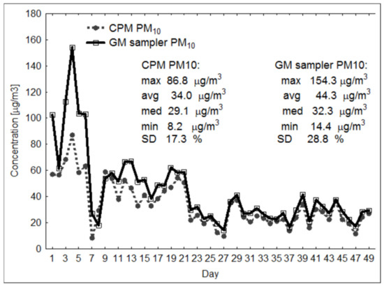
Figure 2.
Average 24 h PM10 mass concentration obtained by two methods in winter campaign.
The variability of PM10 concentration during the observation period in spring is presented in Figure 3. In contrast to the winter period and especially at the beginning of the observation period (early April), the concentrations determined by the two methods were clearly different. A significant difference was also observed in the average values for the whole period. The average concentration of PM10 for the whole measurement period was 29.8 and 49.5 µg/m3 for CPM and GM, respectively. In addition, only two days with exceedances of CPM were recorded, while there were four such days in the case of GM. For both CPM and GM, the coefficient of variation was at almost the same level as it was during the winter period—52% and 67%, respectively. Furthermore, in the case of GM, the relation of PM10 concentration—values of meteorological parameters (Ws, T, P)—was identical to that observed for winter. Such a relationship did not occur for concentrations determined using CPM.
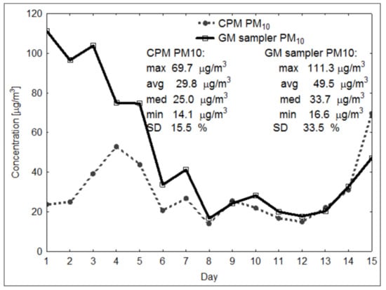
Figure 3.
Average 24 h PM10 mass concentration obtained by two methods in spring campaign.
3.2. Concentration of Elements
Figure 4 shows the full measurement data for PM10-bound elements for the winter period. The mean concentrations of selected elements associated with PM10 ranged widely, with values from 0.61 ng/m3 (Ni) to 219 ng/m3 (Ca) for EDXRF and 1.46 ng/m3 (Ni) to 250 ng/m3 (Ca) for AAS. The masses of the nine elements represented almost 1.6% of the total PM10 mass for EDXRF and 2.0% for AAS. For both techniques, Ca, K and Fe were the most abundant among the determining elements. Toxic trace elements were present in very low concentrations (Ni, Cr, Mn) not exceeding 10 ng/m3 (mean daily value) or low (Pb). The mean concentrations of Ni and Pb in Kotórz Mały did not exceed the permissible values of annual concentrations established by the European Commission (20 ng/m3 and 0.5 µg/m3, respectively; [53]). When considering the position of the median, it may appear that for both methods, the concentrations of Mn, Ni, Zn and Ca can be taken as equivalent. On average over the whole measurement period, the elements associated with the PM10 particulate matter under observation for EDXRF can be ranked as follows: Ca > K > Fe > Zn > Pb > Mn > Cu > Cr > Ni, while for AAS, the order was almost identical: K > Ca > Fe > Zn > Mn > Cu > Cr > Pb > Ni. In the case of EDXRF, two groups of elements can be distinguished because they were characterised by similar coefficients of variation (CV); CV ranging from 52% to 70% (Zn, Cr, Ca, Mn) and CV ranging from 70% to 88% (Pb, K, Fe). Two extreme CVs were also recorded: 39% and 115% for Ni and Cu, respectively. There was much more variability in the elements determined by the AAS method. With the exception of Cr in which the CV was 47%, the concentrations of the other elements showed a significant quartile range, with CVs for Ca, K, Pb, Zn, Cu, Mn, Fe and Ni ranging from 104% to 167%. Significant discrepancies were observed between the results of the two techniques, particularly in the mass concentration of Cr (more than 4 times the median value for AAS) and Cu (more than 3 times the median value for AAS).
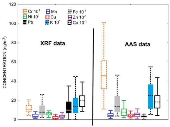
Figure 4.
PM10-bound elements data for winter period. Boxes show the range between the 25th and 75th percentiles. The whiskers extend from the edge of the box to the 5th and 95th percentiles of data. The horizontal line inside indicates the median value.
The full measurement data of PM10-bound elements for the spring period is presented in Figure 5. The mean concentrations of selected elements associated with PM10 ranged widely, with values from 0.82 ng/m3 (Ni) to 472 ng/m3 (Ca) for EDXRF and 1.68 ng/m3 (Pb) to 1718 ng/m3 (Ca) for AAS. The masses of the nine elements represented almost 3.4% of the total PM10 mass for EDXRF and 5.2% for AAS. For both techniques, Ca, K and Fe were the most abundant among the determining elements. From EDXRF data, the mean daily values of toxic trace elements were present in very low concentrations (Ni, Cr, Mn, Pb), not exceeding 10 ng/m3. From AAS data, the mean daily values of toxic trace elements were present in very low concentrations (Ni, Pb), not exceeding 11 ng/m3 or low (Cr, Mn). The mean concentrations of Ni and Pb in Kotórz Mały did not exceed the permissible values of annual concentrations established by the European Commission (20 ng/m3 and 0.5 µg/m3, respectively; European Parliament; European Council, 2008). The position of the median may suggest that for both methods, the Fe and Zn concentrations can be taken as equivalent. Based on an average over the entire measurement period, the PM10-bound elements for EDXRF are ranked as: Ca > Fe > K > Zn > Pb > Mn > Cu > Cr > Ni. In contrast, the order of the elements for AAS is ranked as: Ca > Fe > K > Cu > Zn > Mn > Cr > Ni > Pb. In the case of EDXRF, three groups of elements characterised by a similar coefficient of variation can be distinguished: CV 45% and 53% (Cr, Mn); CV between 62% and 70% (Cu, Zn, Fe); and CV between 79% and 92% (Pb, K, Ca). The maximum variation was in Ni concentration (112%). For the concentrations determined by AAS, in addition to Ca and K (CV 16% and 23%, respectively), more balanced values were observed for Mn, Cu, Ni, Cr and Fe; CV ranged from 51% (Mn) to 65% (Fe). Zn and Pb were in the last group, with CVs of 82% and 84%, respectively. Very significant discrepancies were observed between the results of the two techniques, especially in the mass concentrations of Cu (more than 20-fold higher median value for AAS), Ni (more than 13-fold higher median value for AAS), Cr (more than 8-fold higher median value for AAS), Ca (more than 5-fold higher median value for AAS) and Pb (more than 5-fold higher median value for EDXRF).
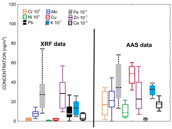
Figure 5.
Data for PM10-bound elements for spring period. Boxes show the range between the 25th and 75th percentiles. The whiskers extend from the edge of the box to the 5th and 95th percentiles of data. The horizontal line inside indicates the median value.
3.3. Meteorological Data
Meteorological data were recorded simultaneously with PM10 and elemental measurements. During the winter campaign, the average temperature was 2 °C, reaching min and max values of −6.9 °C and 9.3 °C, respectively. With the exception of a few days associated with the impact of the cyclone, the pressure was stable and ranged between 996–1046 hPa (mean 1017.6 hPa). The measurement period was dominated by days with very low winds. The movement of air masses was mainly from the NW, S and W directions. The maximum wind velocity was 10.7 m/s, with an average of 4.4 m/s. The total precipitation of 38 mm was lower than the multi-year average. There was no precipitation for 71% of the measurement days. The maximum rainfall was 8.6 mm/h, but the daily average was only 0.8 mm. The average temperature was 6.5 °C during 15 days of measurements in April, reaching daily minimum and maximum values of 1.9 °C and 11.4 °C, respectively. Atmospheric pressure was stable and ranged between 995 and 1015 hPa (mean 1001.3 hPa). Days with very light winds dominated during the measurement period. Air masses moved mainly from the S, SE and NW directions. The maximum wind velocity was 7.4 m/s and the mean was 3.6 m/s. The total precipitation of 13.6 mm was lower than the multi-year average. No precipitation was recorded on 12 of the 15 measurement days. The maximum precipitation was 7.1 mm/h, but the daily average was only 0.9 mm.
4. Discussion
4.1. Comparison of GM and CPM—Concentration of PM10
PM10 concentration values in the vicinity of receptors are determined not only by emission sources but also by the impact of meteorological parameters. Differences in PM10 values may also result from changes in the boundary layer of the atmosphere, which are expressed in different values for temperature, wind speed or precipitation. The analysis of the basic meteorological parameters (Mann-Whitney U test, α = 0.05) registered in the winter as well as spring indicated that there were considerable statistical differences between seasons with regard to the values of T, Ap and Wd (p-value: 0.00; 0.00 and 0.04, respectively) and no considerable statistical differences between seasons with regard to the values of Ws and P (p-value: 0.12; 0.00 and 0.54, respectively).
Table 4 shows the results of the Spearman correlation between PM10 concentration determined with CPM and GM and between PM10 concentration values and recorded meteorological parameters.
Table 4.
Spearman correlation. Relationship between the PM10 concentration and meteorological parameters. Bold values are statistically significant with p = 0.05. Normal font relates to winter data and italic font to spring data.
For both winter and spring periods, a statistically significant, high (spring) and almost full (winter), correlation was obtained between PM10 concentrations determined by both methods. The result of the Wilcoxon test (for p < 0.05) confirmed the consistency of the results from both methods only for the winter period. The p-values of the Wilcoxon test for winter and spring sessions were 0.08 and 0.01, respectively. Thus, hypothesis #1 can only be considered true for the winter campaign period. In the season-to-season comparison (Mann-Whitney U test, p < 0.05), no statistically significant differences were found. In the winter-spring relationship for PM10 concentrations determined by CPM, the test probability was 0.40 and by GM, 0.86.
For both methods, the highest daily PM10 concentration values were obtained in January, which corresponded to negative air temperature, very weak advection and lack of precipitation. Such meteorological conditions significantly did not favour dilution and deposition of pollutants. On the other hand, both in the winter and spring seasons, the lowest PM10 concentrations were observed during days characterised by opposite values of the above meteorological parameters. This may suggest that in the so-called ‘heating season’, local emissions are responsible for air quality in terms of dustiness [19,54].
During the second campaign, significant differences became evident in PM10 concentration values determined by the two methods. It is difficult to explain the reason for a significant disproportion during the first five days of spring measurements. Although there is no correlation between PM10 concentration and wind direction and velocity, the movement of air masses from the S direction (the least numerous buildings—Figure 1) was observed at this time. The CPM aspiration head was distant from the GM head by 18 m to the east. Perhaps this distance was sufficient for the two receptors to be in different air streams, the ‘purer’ (CPM) and more ‘polluted’ (GM). The following facts were also of importance: ideally to the south of the GM aspirator head, there was an outlet of a cyclone serving exhaust from a production hall in a nearby woodwork business; and the GM aspirator was located closer to buildings with active emitters and to home gardens where field work (digging and fertilising beds) was initiated at the end of March. These facts may also have influenced a slightly higher value of PM10 concentration determined by the gravimetric method in the spring campaign compared to the winter one.
For the January–February period, a significant statistical relationship was found in both cases between PM10 concentration and T and P. Similar results regarding the mutual relationship between aerosol concentration and temperature were found in a study in a Czech village [55]. The increase in PM10 concentration corresponded to the intensification of the use of domestic emission sources forced by a decrease in outdoor temperature. At the same time, the occurrence of precipitation (regardless of temperature) effectively reduced the mass of aerosol reaching the receptors. During the spring observations, a clear lack of correlation between PM10 and T is noticeable, which may be due to the fact that the variability of T values during the spring campaign was more than three times lower than in winter. For both full observations, no correlation was found between PM10 concentration and Ap and Wd and Ws. In the last case, there was an exception in winter for GM aspiration.
In comparison with the data received during winter and spring measurement campaigns in different places, results from Kotórz Mały were similar to other small villages, namely Przezchlebie, PL; 67 μg/m3 (winter) and 24 μg/m3 (spring) [45]; Zloukovice, CZ; 38 μg/m3 (spring) [54]; and Brzezina, PL; 80 μg/m3 (winter) [48].
4.2. Comparison of EDXRF and AAS—PM10-Bound Elements
Figure 6 presents the results of the cluster analysis in the form of dendrograms. The clusters were separately created for winter and spring data. Dendrograms were constructed to assess the multidimensional structure of the elemental concentration [56]. The assembled Euclidean distances between the compositional points with clr-transformed coordinates were used to create a dissimilarity matrix. The dendrograms were constructed using Ward’s clustering method. For the winter campaign, there were two clearly distinguished clusters in the dendrogram, with the structure predominantly defined by groups of metals, namely Ca, Fe and K in the first group and Zn, Pb, Cu, Mn, Cr and Ni in the second group. The elements in the first group mainly come from natural sources, including form surface erosion of soils and from plants [18,55,57,58,59]. Elements in the second group are associated with anthropogenic sources, mainly from coal and biomass burning [54,60,61,62,63,64] and from the exploitation of motor vehicles [65,66,67,68,69].
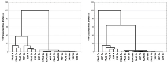
Figure 6.
Dendrograms of the elemental composition of PM10 in relation to the analytical method EDXRF and AAS (winter on the left and spring on the right).
For spring observations, three main clusters were found. At first glance, two of them would be known as winter clusters, but the situation with AAS Ca is interesting and definitely stands out. This is most likely the result of human activity and represents an isolated incident related to local gardening. As mentioned earlier, the GM sampler was located close to domestic gardens where the inhabitants very often fertilised with ground eggshells to enrich the soil.
Table 5 presents a summary of the results of Spearman correlations between elements determined using EDXRF and AAS. Excluding correlations between PM10 concentrations and elements determined in PM10, the winter period data showed a higher number of statistically significant correlations between variables than did the spring data (143 vs. 40, respectively). For the winter period, a statistically significant high correlation (>0.7) was found for seven pairs of variables determined by the EDXRF technique and for 11 pairs of variables determined by the AAS technique. However, for the elements determined by EDXRF, Fe−Mn and Zn−Pb correlations can be described by a linear relationship. For the elements determined by AAS, a linear relationship was found for Zn−Mn and Ca−Mn pairs. In the remaining cases, there were no linear relationships or they were described by a non-monotonic function. For the spring period, statistically significant high correlation was found for 10 pairs of variables determined by the EDXRF technique and for only 1 pair of variables determined by the AAS technique. For the elements determined here by EDXRF, the correlations Fe−Mn, Cr−Ni, K−Mn, Fe−K, Ca−Fe and Ca−K can be described by a linear relationship. In the case of elements determined by the AAS technique, no linear relationships occurred. In other cases, there were no linear relationships or they were described by a non-monotonic function. Considering the correlations of the same elements that were determined by different methods, 6 pairs in the winter period (Cu−Ni, Cu−Cu, Fe−Zn, Zn−Zn, Ni−Pb and K−Ni) had statistically significant high correlations. For the spring period, no statistically significant high correlations were found. In other cases, for example, for statistically significant compounds with respect to elemental composition, some correlations may explain the origin of the aerosol, but it does not seem appropriate to draw specific conclusions from such an analysis.
Table 5.
Spearman correlation. Relationship between the PM10 concentration and meteorological parameters. Bold values are statistically significant with p = 0.05. Normal font relates to winter data and italic font to spring data.
In general, statistically significant correlations of individual element concentrations with PM10 concentrations became apparent in the studies conducted in the winter. High correlations (>0.7) for non-destructive techniques occurred for Fe, Zn, Pb and K. In the case of AAS, such correlations did not occur other than for Cu and Pb. In the spring campaign, for EDXRF, such situations were observed only for Fe, while for AAS, they were observed for Cr, Fe and Ni.
For the purpose of comparison, Table 6 presents the average values of element concentrations in particulate matter determined at different locations. Due to differences in concentration values of particular elements determined by the two different methods, the analytical techniques used by the quoted authors are also given. Attention is drawn by significantly higher concentration values of most analytes compared to the results obtained in rural areas in the Czech Republic and France. The differences most probably result from lower ecological awareness of the Polish rural population and their use of much older and outdated heating systems.
Table 6.
The mean concentration of PM10-bound elements at various sites in the rural area.
Table 6.
The mean concentration of PM10-bound elements at various sites in the rural area.
| Place; Country | Season | Technique | Cr ng/m3 | Mn ng/m3 | Fe ng/m3 | Ni ng/m3 | Cu ng/m3 | Zn ng/m3 | Pb ng/m3 | K ng/m3 | Ca ng/m3 | References |
|---|---|---|---|---|---|---|---|---|---|---|---|---|
| Kotórz Mały, PL | winter | AAS | 4.84 | 9.07 | 222 | 1.46 | 6.49 | 68.6 | 3.36 | 306 | 251 | this study |
| Kotórz Mały, PL | spring | AAS | 18.0 | 22.9 | 421 | 11.0 | 53.3 | 29.3 | 1.68 | 318 | 1719 | this study |
| Kotórz Mały, PL | winter | EDXRF | 1.28 | 4.21 | 114 | 0.61 | 2.44 | 38.4 | 12.9 | 148 | 220 | this study |
| Kotórz Mały, PL | spring | EDXRF | 2.03 | 8.48 | 324 | 0.82 | 2.22 | 32.2 | 10.0 | 164 | 472 | this study |
| Grajów, PL | spring | SSMS | 8.0 | 280 | 19.0 | 12.0 | 80.0 | [46] | ||||
| Przezchlebie, PL | winter | GFAAS | 23.9 | 16.8 | 443 | 4.95 | 11.1 | 135 | 53.4 | [45] | ||
| Przezchlebie, PL | spring | GFAAS | 239.4 | 12.3 | 217 | 6.20 | 2.60 | 72.7 | 20.4 | [45] | ||
| Montagney, FR | winter | ICPMS; INAA | 1.2 | 3.8 | 105 | 1.50 | 4.50 | 23.3 | 9.70 | 267 | 234 | [25] |
| Zloukovice, CZ | spring | ICP-MS | 0.5 | 0.5 | 16.8 | 13.1 | [54] | |||||
| Brzezina, PL | winter | EDXRF | 30 | 40 | 500 | 32.0 | 188 | 85.0 | 648 | 376 | [48] |
Table 7 summarises the results of the Wilcoxon test, which aims to verify the hypotheses stating that: #2—the concentration levels of PM10-bound elements are identical regardless of the method of sampling and analysis; and #3—the concentration levels of PM10 and PM10-bound elements are identical regardless of the season (winter-spring relation). It was suggested in Section 3.2 that the position of the median in Figure 4 and Figure 5 indicates equivalence in concentrations of Mn, Ni, Zn and Ca in winter and Fe and Zn in spring. The results of the Wilcoxon test clearly indicate that these suggestions were true for the observations from the second measurement campaign (in spring) and only for Ca in winter. For the winter campaign, only the contributions of Mn, Ni and Zn to PM10 are equivalent for both techniques. Thus, hypothesis #2 can be considered true only for a very limited range.
Table 7.
EDXRF-AAS p-values of Wilcoxon test for winter and spring sessions. Bold values indicate that the results are significant with p < 0.05.
Hypothesis #3 (Table 8) may be considered true for a much larger range. The levels of PM10 concentrations determined by the compared methods for the winter-spring relationship are very similar. As far as elements are concerned, the comparison of winter and spring results from the EDXRF technique did not provide different results with the exception of chromium and elements of mainly natural origin. In the case of AAS, the hypothesis is true only for potassium.
Table 8.
EDXRF-AAS p-values of Mann-Whitney U test for season-to-season data. Bold values indicate that the results are significant with p < 0.05.
4.3. Identification of Sources of PM10 and PM10-Bound Elements
As previously mentioned, the order of elements during the winter measurement campaign as determined by EDXRF was as follows: Ca > K > Fe > Zn > Pb > Mn > Cu > Cr > Ni. The order was almost identical for AAS: K > Ca > Fe > Zn > Mn > Cu > Cr > Pb > Ni. In spring, the order for EDXRF was Ca > Fe > K > Zn > Pb > Mn > Cu > Cr > Ni; for AAS, it was Ca > Fe > K > Cu > Zn > Mn > Cr > Ni > Pb. Mach et al. [18] presented results from the same receptor and the same apparatus (EDXRF) but they were obtained during the summer campaign. During the summer season, the order of elements in Kotorz Maly was Ca > Fe > K > Zn > Cu > Mn > Cr > Pb > Ni. Comparing only the data from the device (PX-375 Horiba, Osaka, Japan) both in the summer and the spring, the order of the first four and the last place elements was identical (in the winter, the sequence differed slightly). Significant differences appeared in the order of Pb, Mn, Cr and Cu, which may indicate differences in the contribution of individual sources in relation to the warm and cold seasons. In Mach et al. [18], the authors identified five significant sources based on records with an interval of 1 h which determined aero-sanitary conditions in the village in the summer: mineral matter emission, traffic emission, remote low-stack emission, industrial (local and regional) sources and fossil fuel and/or biomass combustion in local households.
Factor analysis (FA) was used to determine the types of sources which were affecting air quality within the receptor. Factor analysis, such as PCA, is a frequently used statistical tool to determine the sources of PM [70,71].
Factor analysis was performed according to the method described by Pohlmann [72]. This was performed by utilising the orthogonal transformation method with Varimax rotation and retention of principal components for which the eigenvalues were close to the unit. The selection of factors was mainly based on Cattell’s scree test [73], whereas the ultimate verification was undertaken by an analysis of residual correlations. Factor loadings indicate the correlation of each element with each component and are related to the source emission composition. In order to avoid the trap of too few variables in relation to the cases, only those elements that showed a high correlation for each method were selected for analysis, that is, Ca, Cu, Fe, Mn and Zn. Elements considered to be derived from both natural and anthropogenic emissions were represented in the tested group.
The eigenvalues of the correlation matrix (Table 9) reflect the significance of the principal components in explaining the information resources of the input variables (percentage share of variation in the dataset). The higher the correlation coefficient of a variable with a component, the more relevant this variable is to the component. In the analysed cases, the first two principal components were decisive for winter (both methods) and spring (EDXRF) and describe 88%, 93.5% and 88.2% of the variability of the original data, respectively. For the analysis of the spring data (AAS), three main factors were identified that explain almost 85% of the variability.
Table 9.
Eigenvalues of the correlation matrix.
The principal components obtained are interpreted on the basis of the values of their coefficients, which are also the coefficients of the linear correlation between the input variables and the principal components. For winter (EDXRF), the first principal component carried almost 72% of the information contained primarily in variables representing elements from natural sources, while the second principal component explained more than 16% of the variation in the data through a variable identified with elements from anthropogenic sources (Table 10). During 49 days of observations, there was no snow cover in Kotórz Mały, indicating that the main source of Mn, Fe and Ca was resuspension from the surface of the fields surrounding the village. Local energy sources of conventional fuel combustion and transport were responsible for Cu and Zn emissions. As for data obtained from AAS analysis, the first principal component carried almost 78% and the second 16% of the information. Here, as in the case from EDXRF data, the same main emission sources can be distinguished, with additional emphasis on the impact of industrial influx emissions, most probably from the Opole cement plant (Cu) [74].
Table 10.
Factor loadings matrix for the PM10 chemical composition obtained after applying the factor analysis.
For spring (EDXRF), the first principal component carried 67.5% and the second 20% of the information. The main sources of emission were transport, surface erosion and low-stack emission from rural household heating. In the case of data collected by AAS analysis, the cumulative explained variance reached almost 85%, with three factors contributing 39.4%, 27.5% and 17.8%, respectively. Here, the same sources as identified for the EDXRF results were responsible for the emissions, with the additional influence of an atypical anthropogenic source, namely fertilisation of soils with ground eggshells (Ca).
5. Conclusions
The results of monitoring PM10 concentrations in a typical rural area during the winter and spring season using two measurement methods (GM and CPM) indicate that:
- -
- The concentrations of PM10 measured by both methods in the winter were equivalent. In the case of the spring season, only after the fifth day of measurements was it observed that the PM10 concentrations were comparable, with both methods indicating the same trend of increase and decrease in PM10 concentrations.
- -
- The lack of significant seasonal differences in PM10 concentrations probably results from the fact that April in Poland is also included in the heating season. Significant changes in PM concentrations were noticeable with the beginning and end of the heating season, which is conventionally assumed to last from 15 October to 25 April.
- -
- Atmospheric conditions had a significant impact on PM10 concentrations. The highest concentrations were recorded at weak advection, lack of precipitation and temperature drop.
Conclusions on the elemental composition analysis of PM10 using two methods (destructive AAS and non-destructive EDXRF) are as follows:
- -
- Both methods showed that Ca, Fe and K had the highest mass shares in PM10 mass both in winter and spring.
- -
- The indications of both methods slightly differed in the case of elements with the lowest share in PM10 mass. In winter, the order for AAS was Cr > Pb > Ni, while in spring, it was Cr > Ni > Pb. For EDXRF, the order was the same for the elements with the lowest concentrations: Cu > Cr > Ni.
- -
- Clear discrepancies were observed in the concentrations of PM10-bound elements in individual seasons. Higher concentrations of PM-bound elements and, thus, higher shares in PM mass were observed in the spring (3.2% for EDXRF; 5.2% for AAS) compared to the winter (1.6% for EDXRF; 2.0% for AAS).
The assessment of the origin of PM10 through factor analysis and the analysis of the correlation between the examined factors showed:
- -
- In winter, the concentration of PM10 and its elemental composition were determined by two components: natural sources (erosion from soil that was not covered with snow at the time of measurement, erosion from plants) and anthropogenic sources, that is, combustion of coal and biomass in home furnaces and combustion of fuel in car engines. In spring, the concentration and elemental composition of PM10 was determined by the two sources indicated above as well as by the local horticultural activity.
- -
- The amount of variance explained by factor analysis varies in both seasons, which suggests a variability in the impact of different emission sources. With the simultaneous influence of several sources or the presence of one dominant source, precise determination of the origin of PM is difficult and requires further analysis.
Comparing the results using different methods (GM vs. CPM and AAS vs. EDXRF) showed that:
- -
- Hypothesis 1 is only true for the winter campaign period.
- -
- Hypothesis 2 can be considered true only for the second measurement campaign in the case of spring measurements and only for Ca in the winter.
- -
- Hypothesis 3 may be considered true for PM10 and PM10-bound elements with the exception of chromium and crustal elements for EDXRF. For AAS, the hypothesis is true only for potassium.
In order to compare the results obtained with different methods, it is necessary to ensure that both types of measuring and sampling equipment are located directly next to each other. The conducted research indicated that even a small distance (18 m in this study) may influence the variability of the results.
The conducted measurements and analysis of the results indicate a plan for further research, which should also include the fine PM fraction, for example, PM2.5. The fine particles are more enriched in trace elements (Cr, Ni, Pb, Cu) than in coarse. Analysis of fine PM could provide additional information on the origin of the PM at the receptor as well as the equivalence of the methods. The results obtained in this study do not exclude any of the proposed methods for the determination of concentrations and elemental composition, as both provided similar conclusions regarding the origin of PM10 in the receptor. Although the measurement method and its equivalence to the reference method prove the reliability of the results, an important source of information about the factors influencing these results requires a detailed correlation analysis, for example, between concentrations of elements and atmospheric conditions as well as the source apportionment using the methods of factor analysis (FA), principal components analysis (PCA) or positive matrix factorisation (PMF). A limitation for a complete analysis of the problem was the low number of records collected (for the spring season). The authors plan further research in this area, devoted to improving the accuracy of the quantitative analysis. A dedicated calibration procedure will be further developed to obtain accurate and more precise results.
Author Contributions
Conceptualization, T.M., T.O., W.R.-K., J.R., P.R.-K. and G.M.; Formal analysis, M.B. and A.K.; Investigation, T.M. and T.O.; Methodology, T.M., T.O., W.R.-K. and G.M.; Resources, T.M. and T.O.; Supervision, J.R.; Validation, J.R. and Z.Z.; Writing—Original draft, T.M., T.O. and K.B.; Writing—Review & editing, W.R.-K. and Z.Z. All authors have read and agreed to the published version of the manuscript.
Funding
The project was funded with private initiative.
Informed Consent Statement
Not applicable.
Acknowledgments
The authors wish to kindly thank Krystyna Wieczorek and Wacław Siudyła for their help in conducting surveys among the residents of Kotórz Mały. The authors also wish to kindly thank the authorities of the Mechanics Department of the Opole University of Technology for financial support, without which it would not have been possible to carry out this research project. The authors would like to give special thanks to Piotr Długosz for allowing the research apparatus to be located on his property and for providing a source of electricity.
Conflicts of Interest
The authors declare they have no conflict of interest and no financial interests.
Statements & Declarations
All authors declare that they have met all ethical criteria and have agreed to participate in the publication. All authors have read and agreed to the published version of the manuscript. The authors declare the availability of data and materials.
Compliance with Ethical Standards
The authors declare that no studies involving humans and/or animals were carried out.
References
- Wang, J.; Pan, Y.; Tian, S.; Chen, X.; Wang, L.; Wang, Y. Size distributions and health risks of particulate trace elements in rural areas in northeastern China. Atmos. Res. 2016, 168, 191–204. [Google Scholar] [CrossRef]
- Roy, D.; Seo, Y.-C.; Kim, S.; Oh, J. Human health risk assessment for airborne PM10-bound metals in Seoul, Korea. Env. Sci Pollut. Res. 2019, 26, 24247–24261. [Google Scholar] [CrossRef]
- Crilley, L.R.; Lucarelli, F.; Bloss, W.J.; Harrison, R.M.; Beddows, D.C.; Calzolai, G.; Nava, S.; Valli, G.; Bernardoni, V.; Vecchi, R. Source apportionment of fine and coarse particles at a roadside and urban background site in London during the 2012 summer ClearfLo campaign. Environ. Pollut. 2017, 220, 766–778. [Google Scholar] [CrossRef] [PubMed] [Green Version]
- Santos, M.L.O.; Santos, K.M.B.; França, E.J. Comparison Between Edxrf and Faas for Zn Determination in Terrestrial Mollusks. In Proceedings of the 2015 International Nuclear Atlantic Conferen, São Paulo, Brazil, 4–9 October 2015; p. 7. [Google Scholar]
- Visser, S.; Slowik, J.G.; Furger, M.; Zotter, P.; Bukowiecki, N.; Canonaco, F.; Flechsig, U.; Appel, K.; Green, D.C.; Tremper, A.H.; et al. Advanced source apportionment of size-resolved trace elements at multiple sites in London during winter. Atmos. Chem. Phys. 2015, 15, 11291–11309. [Google Scholar] [CrossRef] [Green Version]
- Venter, A.D.; Van Zyl, P.G.; Beukes, J.P.; Josipovic, M.; Hendriks, J.; Vakkari, V.; Laakso, L. Atmospheric trace metals measured at a regional background site (Welgegund) in South Africa. Atmos. Chem. Phys. 2017, 17, 4251–4263. [Google Scholar] [CrossRef] [Green Version]
- Tahri, M.; Benchrif, A.; Bounakhla, M.; Benyaich, F.; Noack, Y. Seasonal variation and risk assessment of PM2.5 and PM2.5-10 in the ambient air of Kenitra, Morocco. Environ. Sci. Process. Impacts 2017, 19, 1427–1436. [Google Scholar] [CrossRef]
- Enamorado-Báez, S.M.; Gómez-Guzmán, J.M.; Chamizo, E.; Abril, J.M. Levels of 25 trace elements in high-volume air filter samples from seville (2001–2002): Sources, enrichment factors and temporal variations. Atmos. Res. 2015, 155, 118–129. [Google Scholar] [CrossRef] [Green Version]
- Contini, D.; Cesari, D.; Donateo, A.; Chirizzi, D.; Belosi, F. Characterization of PM10 And PM2.5 and their metals content in different typologies of sites in South-Eastern Italy. Atmosphere 2014, 5, 435–453. [Google Scholar] [CrossRef] [Green Version]
- Canepari, S.; Astolfi, M.L.; Farao, C.; Maretto, M.; Frasca, D.; Marcoccia, M.; Perrino, C. Seasonal variations in the chemical composition of particulate matter: A case study in the Po Valley. Part II: Concentration and solubility of micro- and trace-elements. Environ. Sci. Pollut. Res. 2014, 21, 4010–4022. [Google Scholar] [CrossRef]
- Alleman, L.Y.; Lamaison, L.; Perdrix, E.; Robache, A.; Galloo, J.C. PM10 metal concentrations and source identification using positive matrix factorization and wind sectoring in a French industrial zone. Atmos. Res. 2010, 96, 612–625. [Google Scholar] [CrossRef]
- Zunic, B.; Peter, S. World’s largest Science, Technology & Medicine Open Access Book Publisher; INTECH: Houston, TX, USA, 2018; pp. 267–322. [Google Scholar]
- Ukaogo, P.O.; Ewuzie, U.; Onwuka, C.V. Environmental pollution: Causes, effects, and the remedies. In Microorganisms for Sustainable Environment and Health; Elsevier: Amsterdam, The Netherlands, 2020; ISBN 9780128190012. [Google Scholar]
- Yadav, I.C.; Devi, N.L. Biomass burning, regional air quality, and climate change. In Encyclopedia of Environmental Health; Elsevier: Amsterdam, The Netherlands, 2019; ISBN 9780444639523. [Google Scholar]
- Coronas, M.V.; Bavaresco, J.; Rocha, J.A.V.; Geller, A.M.; Caramão, E.B.; Rodrigues, M.L.K.; Vargas, V.M.F. Attic dust assessment near a wood treatment plant: Past air pollution and potential exposure. Ecotoxicol. Environ. Saf. 2013, 95, 153–160. [Google Scholar] [CrossRef] [PubMed]
- Majewski, G.; Rogula-Kozlowska, W.; Rozbicka, K.; Rogula-Kopiec, P.; Mathews, B.; Brandyk, A. Concentration, chemical composition and origin of PM1: Results from the first long-term measurement campaign in Warsaw (Poland). Aerosol Air Qual. Res. 2018, 18, 636–654. [Google Scholar] [CrossRef] [Green Version]
- Rogula-Kozłowska, W.; Majewski, G.; Błaszczak, B.; Klejnowski, K.; Rogula-Kopiec, P. Origin-Oriented Elemental Profile of Fine Ambient Particulate Matter in Central European Suburban Conditions. Int. J. Environ. Res. Public Health 2016, 13, 715. [Google Scholar] [CrossRef] [PubMed] [Green Version]
- Mach, T.; Rogula-Kozłowska, W.; Bralewska, K.; Majewski, G.; Rogula-Kopiec, P.; Rybak, J. Impact of municipal, road traffic and natural sources on PM10: The hourly variability at a rural site in Poland. Energies 2021, 14, 2654. [Google Scholar] [CrossRef]
- Olszowski, T. Influence of individual household heating on PM2.5 concentration in a rural settlement. Atmosphere 2019, 10, 782. [Google Scholar] [CrossRef] [Green Version]
- Błaszczyk, E.; Rogula-Kozłowska, W.; Klejnowski, K.; Fulara, I.; Mielżyńska-Švach, D. Polycyclic aromatic hydrocarbons bound to outdoor and indoor airborne particles (PM2.5) and their mutagenicity and carcinogenicity in Silesian kindergartens, Poland. Air Qual. Atmos. Heal. 2016, 10, 389–400. [Google Scholar] [CrossRef] [Green Version]
- Khoshsima, M.; Ahmadi-Givi, F.; Bidokhti, A.A.; Sabetghadam, S. Impact of meteorological parameters on relation between aerosol optical indices and air pollution in a sub-urban area. J. Aerosol Sci. 2014, 68, 46–57. [Google Scholar] [CrossRef]
- Massey, D.D.; Kulshrestha, A.; Taneja, A. Particulate matter concentrations and their related metal toxicity in rural residential environment of semi-arid region of India. Atmos. Environ. 2013, 67, 278–286. [Google Scholar] [CrossRef]
- Grange, S.K.; Salmond, J.A.; Trompetter, W.J.; Davy, P.K.; Ancelet, T. Effect of atmospheric stability on the impact of domestic wood combustion to air quality of a small urban township in winter. Atmos. Environ. 2013, 70, 28–38. [Google Scholar] [CrossRef]
- Maenhaut, W.; Vermeylen, R.; Claeys, M.; Vercauteren, J.; Matheeussen, C.; Roekens, E. Assessment of the contribution from wood burning to the PM10 aerosol in Flanders, Belgium. Sci. Total Environ. 2012, 437, 226–236. [Google Scholar] [CrossRef]
- Gaudry, A.; Moskura, M.; Mariet, C.; Ayrault, S.; Denayer, F.; Bernard, N. Inorganic pollution in PM10 particles collected over three French sites under various influences: Rural conditions, traffic and industry. Water Air Soil Pollut. 2008, 193, 91–106. [Google Scholar] [CrossRef]
- Khedairia, S.; Khadir, M.T. Impact of clustered meteorological parameters on air pollutants concentrations in the region of Annaba, Algeria. Atmos. Res. 2012, 113, 89–101. [Google Scholar] [CrossRef]
- European Commission. Ambient Air Pollution by AS, CD and NI Compounds; European Commission: Luxembourg, 2000; ISBN 9289420545. [Google Scholar]
- Bilo, F.; Borgese, L.; Wambui, A.; Assi, A.; Zacco, A.; Federici, S.; Eichert, D.M.; Tsuji, K.; Lucchini, R.G.; Placidi, D.; et al. Comparison of multiple X-ray fluorescence techniques for elemental analysis of particulate matter collected on air filters. J. Aerosol Sci. 2018, 122, 1–10. [Google Scholar] [CrossRef] [PubMed]
- Diapouli, E.; Manousakas, M.; Vratolis, S.; Vasilatou, V.; Maggos, T.; Saraga, D.; Grigoratos, T.; Argyropoulos, G.; Voutsa, D.; Samara, C.; et al. Evolution of air pollution source contributions over one decade, derived by PM10 and PM2.5 source apportionment in two metropolitan urban areas in Greece. Atmos. Environ. 2017, 164, 416–430. [Google Scholar] [CrossRef]
- Lomboy, M.F.T.C.; Quirit, L.L.; Molina, V.B.; Dalmacion, G.V.; Schwartz, J.D.; Suh, H.H.; Baja, E.S. Characterization of particulate matter 2.5 in an urban tertiary care hospital in the Philippines. Build. Environ. 2015, 92, 432–439. [Google Scholar] [CrossRef]
- López-García, P.; Gelado-Caballero, M.D.; Collado-Sánchez, C.; Hernández-Brito, J.J. Solubility of aerosol trace elements: Sources and deposition fluxes in the Canary Region. Atmos. Environ. 2017, 148, 167–174. [Google Scholar] [CrossRef]
- Nair, P.R.; George, S.K.; Sunilkumar, S.V.; Parameswaran, K.; Jacob, S.; Abraham, A. Chemical composition of aerosols over peninsular India during winter. Atmos. Environ. 2006, 40, 6477–6493. [Google Scholar] [CrossRef]
- Galvão, E.S.; Santos, J.M.; Lima, A.T.; Reis, N.C.; Orlando, M.T.D.A.; Stuetz, R.M. Trends in analytical techniques applied to particulate matter characterization: A critical review of fundaments and applications. Chemosphere 2018, 199, 546–568. [Google Scholar] [CrossRef]
- Bizo, M.L.; Roba, C.; Levei, E.A.; Hoaghia, M.A.; Modoi, C.O.; Ozunu, A. Comparison of FAAS and XRF performance for metal monitoring in brownfields. Environ. Eng. Manag. J. 2015, 14, 2515–2521. [Google Scholar] [CrossRef]
- Custódio, P.J.; Pessanha, S.; Pereira, C.; Carvalho, M.L.; Nunes, M.L. Comparative study of elemental content in farmed and wild life Sea Bass and Gilthead Bream from four different sites by FAAS and EDXRF. Food Chem. 2011, 124, 367–372. [Google Scholar] [CrossRef]
- Mäkinen, E.; Korhonen, M.; Viskari, E.L.; Haapamäki, S.; Järvinen, M.; Lu, L.I. Comparison of XRF and FAAS methods in analysing CCA contaminated soils. Water Air Soil Pollut. 2006, 171, 95–110. [Google Scholar] [CrossRef]
- Morley, J.C.; Clark, C.S.; Deddens, J.A.; Ashley, K.; Roda, S. Evaluation of a portable X-ray fluorescence instrument for the determination of lead in workplace air samples. Appl. Occup. Environ. Hyg. 1999, 14, 306–316. [Google Scholar] [CrossRef] [PubMed]
- Sterling, D.A.; Lewis, R.D.; Luke, D.A.; Shadel, B.N. A portable X-ray fluorescence instrument for analyzing dust wipe samples for lead: Evaluation with field samples. Environ. Res. 2000, 83, 174–179. [Google Scholar] [CrossRef]
- Mohammed, H.; Sadeek, S.; Mahmoud, A.R.; Zaky, D. Comparison of AAS, EDXRF, ICP-MS and INAA performance for determination of selected heavy metals in HFO ashes. Microchem. J. 2016, 128, 1–6. [Google Scholar] [CrossRef]
- Gerboles, M.; Buzica, D.; Alleman, L.; Pfeffer, U.; Gladtke, D.; Olschewski, A.; Leary, B.O.; Pockeviciute, D.; Tursic, J.; Yardley, R. Intercomparison Exercise for Heavy Metals in PM 10; European Commission: Luxembourg, 2008; ISBN 9789279082061. [Google Scholar]
- Yatkin, S.; Belis, C.A.; Gerboles, M.; Calzolai, G.; Lucarelli, F.; Cavalli, F.; Trzepla, K. An interlaboratory comparison study on the measurement of elements in PM10. Atmos. Environ. 2016, 125, 61–68. [Google Scholar] [CrossRef]
- Gupta, S.; Soni, P.; Gupta, A.K. Optimization of WD-XRF analytical technique to measure elemental abundance in PM2.5 dust collected on quartz-fibre filter. Atmos. Pollut. Res. 2021, 12, 345–351. [Google Scholar] [CrossRef]
- Osán, J.; Börcsök, E.; Czömpöly, O.; Dian, C.; Groma, V.; Stabile, L.; Török, S. Experimental evaluation of the in-the-field capabilities of total-reflection X-ray fluorescence analysis to trace fine and ultrafine aerosol particles in populated areas. Spectrochim. Acta Part B 2020, 167, 105852. [Google Scholar] [CrossRef]
- Bartley, D.L.; Slaven, J.E.; Rose, M.C.; Andrew, M.E.; Harper, M. Uncertainty determination for nondestructive chemical analytical methods using field data and application to XRF analysis for lead. J. Occup. Environ. Hyg. 2007, 4, 931–942. [Google Scholar] [CrossRef]
- Mainka, A.; Zajusz-Zubek, E.; Kaczmarek, K. PM10 composition in urban & rural nursery schools in Upper Silesia, Poland: A trace elements analysis. Int. J. Environ. Pollut. 2017, 61, 98. [Google Scholar] [CrossRef]
- Konarski, P.; Hałuszka, J.; Ćwil, M. Comparison of urban and rural particulate air pollution characteristics obtained by SIMS and SSMS. Appl. Surf. Sci. 2006, 252, 7010–7013. [Google Scholar] [CrossRef]
- Olszowski, T.; Tomaszewska, B.; Góralna-Włodarczyk, K. Air quality in non-industrialised area in the typical Polish countryside based on measurements of selected pollutants in immission and deposition phase. Atmos. Environ. 2012, 50, 139–147. [Google Scholar] [CrossRef]
- Samek, L.; Zwoździak, A.; Sówka, I. Chemical characterization and source identification of particulate matter pm 10 in a rural and urban site in poland. Environ. Prot. Eng. 2013, 39, 91–103. [Google Scholar] [CrossRef]
- Austrian Standards Institute Ambient Air—Standard Gravimetric Measurement Method for Hte Determination of the PM10 or PM2. 5 Mass Concentration of Suspended Particulate Matter; Austrian Standards Institute: Vienna, Austria, 2012. [Google Scholar]
- Scheme, A.; Laboratories, F.O.R. SAC-SINGLAS A Guide on Measurement Uncertainty in Chemical & Microbiological Analysis. 2008. Available online: https://fdocuments.in/document/a-guide-on-measurement-uncertainty-in-chemical-guide-on-measurement-uncertainty.html?page=1 (accessed on 8 September 2021).
- Liberti, A. Modern methods for air pollution monitoring. Pure Appl. Chem. 1975, 44, 519–534. [Google Scholar] [CrossRef] [Green Version]
- Castro, A.; Alonso-Blanco, E.; González-Colino, M.; Calvo, A.I.; Fernández-Raga, M.; Fraile, R. Aerosol size distribution in precipitation events in León, Spain. Atmos. Res. 2010, 96, 421–435. [Google Scholar] [CrossRef]
- European Parliament. European Council Directive 2008/50/EC on ambient air quality and cleaner air for Europe. Off. J. Eur. Communities 2008. Available online: https://ec.europa.eu/environment/archives/cafe/pdf/cafe_dir_en.pdf (accessed on 9 May 2021).
- Braniš, M.; Domasová, M.; Řezáčová, P. Particulate air pollution in a small settlement: The effect of local heating. Appl. Geochem. 2007, 22, 1255–1264. [Google Scholar] [CrossRef]
- Jandačka, D.; Ďurčanská, D. Air Pollution by Gases and PM in Rural Areas. Trans. Transp. Sci. 2014, 7, 143–152. [Google Scholar] [CrossRef] [Green Version]
- Kaufman, L.; Rousseeuw, P. Finding Groups in Data: An Introduction to Cluster Analysis; John Wiley & Sons: Hoboken, NJ, USA, 2009. [Google Scholar]
- Kim, M.K.; Jo, W.K. Elemental composition and source characterization of airborne PM10 at residences with relative proximities to metal-industrial complex. Int. Arch. Occup. Environ. Health 2006, 80, 40–50. [Google Scholar] [CrossRef]
- Pan, Y.; Wang, Y.; Sun, Y.; Tian, S.; Cheng, M. Size-resolved aerosol trace elements at a rural mountainous site in Northern China: Importance of regional transport. Sci. Total Environ. 2013, 461–462, 761–771. [Google Scholar] [CrossRef]
- Pant, P.; Harrison, R.M. Critical review of receptor modelling for particulate matter: A case study of India. Atmos. Environ. 2012, 49, 1–12. [Google Scholar] [CrossRef] [Green Version]
- Jandacka, D.; Durcanska, D. Differentiation of particulate matter sources based on the chemical composition of PM10 in functional urban areas. Atmosphere 2019, 10, 583. [Google Scholar] [CrossRef] [Green Version]
- Pant, P.; Harrison, R.M. Estimation of the contribution of road traffic emissions to particulate matter concentrations from field measurements: A review. Atmos. Environ. 2013, 77, 78–97. [Google Scholar] [CrossRef]
- Samek, L. Source apportionment of the PM10 fraction of particulate matter collected in Kraków, Poland. Nukleonika 2012, 57, 601–606. [Google Scholar]
- Khare, P.; Baruah, B.P. Elemental characterization and source identification of PM2.5 using multivariate analysis at the suburban site of North-East India. Atmos. Res. 2010, 98, 148–162. [Google Scholar] [CrossRef]
- Rajšić, S.; Mijić, Z.; Tasić, M.; Radenković, M.; Joksić, J. Evaluation of the levels and sources of trace elements in urban particulate matter. Environ. Chem. Lett. 2008, 6, 95–100. [Google Scholar] [CrossRef]
- Kuo, C.Y.; Wang, J.Y.; Liu, W.T.; Lin, P.Y.; Tsai, C.T.; Cheng, M.T. Evaluation of the vehicle contributions of metals to indoor environments. J. Expo. Sci. Environ. Epidemiol. 2012, 22, 489–495. [Google Scholar] [CrossRef]
- Richter, P.; Griño, P.; Ahumada, I.; Giordano, A. Total element concentration and chemical fractionation in airborne particulate matter from Santiago, Chile. Atmos. Environ. 2007, 41, 6729–6738. [Google Scholar] [CrossRef]
- Sternbeck, J.; Sjödin, Å.; Andréasson, K. Metal emissions from road traffic and the influence of resuspension—Results from two tunnel studies. Atmos. Environ. 2002, 36, 4735–4744. [Google Scholar] [CrossRef]
- Toscano, G.; Moret, I.; Gambaro, A.; Barbante, C.; Capodaglio, G. Distribution and seasonal variability of trace elements in atmospheric particulate in the Venice Lagoon. Chemosphere 2011, 85, 1518–1524. [Google Scholar] [CrossRef] [Green Version]
- Kulshrestha, A.; Satsangi, P.G.; Masih, J.; Taneja, A. Metal concentration of PM2.5 and PM10 particles and seasonal variations in urban and rural environment of Agra, India. Sci. Total Environ. 2009, 407, 6196–6204. [Google Scholar] [CrossRef]
- Escrig Vidal, A.; Monfort, E.; Celades, I.; Querol, X.; Amato, F.; Minguillón, M.C.; Hopke, P.K. Application of optimally scaled target factor analysis for assessing source contribution of ambient PM10. J. Air Waste Manag. Assoc. 2009, 59, 1296–1307. [Google Scholar] [CrossRef]
- Kavouras, I.G.; Koutrakis, P.; Cereceda-Balic, F.; Oyola, P. Source apportionment of PM10 and PM2.5 in five Chilean cities using factor analysis. J. Air Waste Manag. Assoc. 2001, 51, 451–464. [Google Scholar] [CrossRef] [PubMed]
- Pohlmann, J.T. Use and Interpretation of Factor Analysis in ‘The Journal of Educational Research’: 1992–2002. J. Educ. Res. 2004, 98, 14–22. [Google Scholar] [CrossRef]
- Cattell, R.B. The scree test for the number of factors. Multivar. Behav. Res. 1966, 1, 245–276. [Google Scholar] [CrossRef] [PubMed]
- Fernández-Camacho, R.; Rodríguez, S.; de la Rosa, J.; Sánchez de la Campa, A.M.; Alastuey, A.; Querol, X.; González-Castanedo, Y.; Garcia-Orellana, I.; Nava, S. Ultrafine particle and fine trace metal (As, Cd, Cu, Pb and Zn) pollution episodes induced by industrial emissions in Huelva, SW Spain. Atmos. Environ. 2012, 61, 507–517. [Google Scholar] [CrossRef] [Green Version]
Publisher’s Note: MDPI stays neutral with regard to jurisdictional claims in published maps and institutional affiliations. |
© 2022 by the authors. Licensee MDPI, Basel, Switzerland. This article is an open access article distributed under the terms and conditions of the Creative Commons Attribution (CC BY) license (https://creativecommons.org/licenses/by/4.0/).