Abstract
In modern Electric Power Systems, emphasis is placed on the increasing share of electricity from renewable energy sources (PV, wind, hydro, etc.), at the expense of energy generated with the use of fossil fuels. This will lead to changes in energy supply. When there is excessive generation from RESs, there will be too much energy in the system, otherwise, there will be a shortage of energy. Therefore, smart devices should be introduced into the system, the operation of which can be initiated by the conditions of the power grid. This will allow the load profiles of the power grid to be changed and the electricity supply to be used more rationally. The article proposes an elastic energy management algorithm (EEM) in a hierarchical control system with distributed control devices for controlling domestic smart appliances (SA). In the simulation part, scenarios of the algorithm’s operation were carried out for 1000 households with the use of the distribution of activities of individual SAs. In experimental studies, simplified results for three SA types and 100 devices for each type were presented. The obtained results confirm that, thanks to the use of SAs and the appropriate algorithm for their control, it is possible to change the load profile of the power grid. The efficacious operation of SAs will be possible thanks to the change of habits of electricity users, which is briefly described in the article.
1. Introduction
A number of countries have different approaches to problems related to sustainable development and environmental protection. The European Union (EU) countries have one of the most developed plans and strategies in this area. The European Commission has committed to achieving climate neutrality by 2050, as described in the documents of the “European Green Deal” [1]. Part of the European Green Deal is the “Fit for 55” package. Its aim is to put the EU firmly on the path to climate neutrality by 2050. The “Fit for 55” package envisages a revision of the Renewable Energy Directive (RED II) [2]. This change is expected to help the EU meet its new 55% greenhouse gas emissions target. The revised RED II directive sets a new EU target of at least 40% of the share of renewable energy in final energy consumption by 2030. Meeting these requirements will require the connection of a significant number of renewable energy sources (RES) to the distribution network. The RES energy generation profile is periodic and depends on weather conditions [3]. On the other hand, the reduction of greenhouse gases will result in the shutdown of a large number of conventional fossil fuel power plants processing brown coal, hard coal and petroleum [4]. Such a situation may lead to a very high generation of energy from renewable sources in favorable weather conditions, e.g., from Photovoltaic Panels (PV) on a sunny day. Such production will exceed the energy demand. In contrast, during unfavorable weather conditions, there will be a shortage of energy in the system, because RESs will not generate it. Additionally, solar energy from PVs will be available only during the day-time hours, and it will not be available in the morning, evening and night-time hours. The complementarity of PV and wind turbine energy generation may also not meet the energy demand. To meet the energy demand, either very expensive energy storage systems (ESS) [5] or fossil fuel generators with a high rate of inclusion should be used, e.g., gas microturbines. The geopolitical situation in Europe may mean that gas resources may not be sufficient to balance the electricity system with a large amount of RESs.
Figure 1 shows power measurements for one week, illustrating the load time courses for 110/15 kV substations, and a comparison with the generation profile of a PV installation with the power planned for installation in a given MV line. The overproduction of energy from the PV system is marked in green. This energy should be stored [6], used or sent to places where there is a demand [7]. As can be seen from the presented figure, the energy generated by PVs is unstable over time. During one week, there were days with very little, very high, and extremely variable energy outputs all day long, or with instantaneous energy bursts in production. Prosumer photovoltaic systems installed on buildings show a similar behavior. In the local balancing of the system, it is necessary to use/store as much energy as possible from both local prosumer low-voltage installations and large photovoltaic power plants connected to the MV.
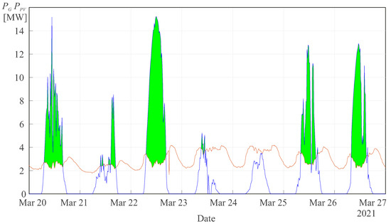
Figure 1.
Sample measurement result in 110/15 kV substations; red: energy consumption from the transformer; blue: potential PV power generation, including sources to be connected in the future; the wave forms of PV generation were determined on the basis of measurements from a 1 MWp power plant; green field: energy that must be sent to the power grid to other loads or stored in the ESS.
The demand for electricity and the penetration of small-scale distributed generators are rapidly growing in LV distribution networks, thus, the existing electrical systems will need future adjustments. Inverters for distributed energy resources (DERs) have been released with standards and grid codes for interconnection with the distribution grid. To include increased DER penetration and optimize DER value in the grid, the new standard and grid codes anticipate that DERs will perform a range of power system support roles. The following are more widespread measures to detect violations of the upper voltage limit: voltage and reactive power control by PV inverters, demand response (DR) and storage.
One of the conceptual approaches to using energy overproduction is to manage energy demand in such a way that its consumption is as high as possible at times of high generation. Local self-consumption should be increased during a large surplus of energy production from RESs, and self-consumption should be reduced during an energy shortage in the system [8]. There are many concepts employed in controlling the demand for electricity by the use of a smart appliances (SA) described in the scientific literature. This article will present the concept of using and integrating smart home devices and consumer devices (e.g., electric vehicles [9], small energy storage) for energy balancing in a local low-voltage distribution system. An algorithm for elastic energy management will be proposed which takes into account the priorities of device operation set by the user. In order for such an energy management system to function properly, it should have information about the operating status of the system, i.e., the overproduction/shortage of energy in the system.
There are many solutions for the control of the demand for electricity in the scientific literature. Here, a brief overview of selected applications for use with home appliances will be provided. An interesting solution to the problem of excessive grid load was presented in [10]. The proposed Smart Home energy management system takes into account network constraints and user priorities. It is based on a heuristic technique for the device scheduling process. The limitation of this approach is the necessity to have information about the power available from the grid and about the power generated from RESs. As there is no single leading signal about the state of the power system, the system is quite complex. In another article [11], the predictive control model for optimal energy management in a district, involving buildings with vertically placed photovoltaic systems integrated into the building and energy storage systems, is discussed. The proposed control strategy aims to maximize the district’s independence from the external power grid, which is achieved through the collaboration of interactive buildings. The proposed control scheme includes components such as forecast, optimizer and load in the form of the analyzed district. Another concept of energy management is presented in [12], which includes a comparative study of two home micro-grids, one of which is a vehicle-to-home network. Electric vehicle integration makes an economic contribution by reducing costs, supporting other MG components and reducing the load on the main network. The next publication [13] presents an overview of the most recent literature on residential household energy management, especially holistic solutions, and proposes new viewpoints on residential appliance scheduling in smart homes.
Due to the stochastic nature of RES generation, and in order to ensure the stable operation of the system, an increase in the number of control points and control devices must be achieved, which will significantly increase the burden on the system operator at the secondary control level. Therefore, a decentralized energy management and control system should be installed in the customer’s system. Then, in such a system, information on regulatory needs will either be provided by the distribution system operator or it will be obtained from local measurement points. A hierarchical control system has been proposed, as shown in Figure 2 [14].
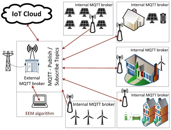
Figure 2.
Proposed hierarchical control system.
The simplest solution for a hierarchical control system is a structure with a local central unit located in an MV/LV transformer station. Information on production from large generating units (wind or PV) connected to the MV is provided to the central management unit, e.g., via Wi-Fi or other communication protocols. Additionally, information about the energy production from the RESs is sent to the central unit, if possible. This information can be taken directly from an intelligent energy meter, solar inverter or other device providing information about the generation level of prosumer sources. Information about the amount of energy in the grid can also be obtained from the voltage level of the consumer grid [8,15]. When there is a need to increase energy consumption or reduce it, the central management unit sends a signal to distributed control devices (DCD) located in a given building or at a location. All kinds of information exchange between individual units are realized using the Message Queue Telemetry Transport (MQTT) protocol. This protocol is based on published and subscribed topic patterns. Such a use of the MQTT protocol makes it possible to subscribe only to those data on topics that are essential for the operation of a given unit in the proposed hierarchical control system with DCDs. The role of the server with which clients will connect to publish topics for individual DCDs is performed by the MQTT broker. For the proposed hierarchical control system with DCDs, external and internal MQTT brokers are distinguished. Such an approach enables grouping of data from a given DCD. In the internal MQTT broker, topics may be grouped on energy consumption, e.g., on the level of one household and energy generation from RESs. The energy consumption can be the total value of the energy consumed by all devices, or it can also be grouped for individual devices of energy consumers. The greatest possibilities for providing additional data on configuration possibilities will be offered by SAs. For SAs, it is possible to read the current energy consumption and assess the possibility of modifying the behavior of a given SA. In this case, the modification will be to change the power level. The scope of possibilities for changing the power will result from the parameters set by the manufacturer of a given SA. The possibility of communication between the proposed hierarchical control system with the DCD and other hierarchical control systems is provided by the use of solutions based on the concept of the Internet of Things (IoT) with a cloud function. In this case, IoT Cloud solutions can be based on one of the following solutions: AWS IoT [16], Google Cloud IoT [17], IBM Cloud IoT [18], Microsoft Azure IoT [19], Oracle IoT Cloud Service [20] or others.
To summarize the above, in the proposed hierarchical control, different system communication tasks can be distinguished. Some of these tasks play a measuring, controlling or measuring and controlling role. Measurement tasks involve collecting data on the current demand for and supply of energy. Data is provided from internal MQTT brokers. The control or measurement and control tasks concern the transfer of guidelines on the method of controlling a given intelligent device by the EEM algorithm. In addition, there are also tasks related to maintaining the correct functioning of the hierarchical control system. In this case, the tasks will concern the verification of the status of a given device. The tasks also include tasks related to ensuring the security level, such as system access control.
The DCD is also responsible for reacting to changes in the voltage. After exceeding the range defined by the formula:
actions are taken through the use of a dedicated algorithm. The proposed algorithm for the Elastic Energy Management (EEM) is implemented in DCD. The DCD communicates with individual smart appliances in order to achieve the set goal of reducing or increasing energy consumption [8]. For the proper operation of the EEM algorithm, all necessary data on energy consumption or generation will be provided from an external MQTT broker. The main aim of the article is to present the concept of an electricity management system in a smart home using SAs.
The innovative part of the research results presented in the article is the ensuring of the use of the EEM algorithm to respond to an overvoltage in the smart grid and to define user behavior and the means to model virtually any user device. Such innovation allows the creation of virtual device prototypes to evaluate their energy efficiency properties. Verification of the correctness of the assumptions was made based on the Probability Density Function (PDF) and the estimator PDF. Research studies have been conducted on datasets describing user behavior in an exemplary 1000-household study. The presented considerations take into account the IoT technology for data exchange between devices in the Smart Grid network.
The paper is organized as follows: Section 2 presents the Elastic Energy Management algorithm, Section 3 describes the simulation research conducted, Section 4 presents smart appliance functionality and user behavior, Section 5 includes assumptions and results for the conducted experimental results, and Section 6 includes the conclusions of this study.
2. The Elastic Energy Management Algorithm
In order to manage the demand and supply of energy in DCDs through EEM, it was necessary to define the parameters of the model. For this purpose, it was defined as:
The requirement for individual parameters of each SA is to have defined properties. The properties of a given SA are determined on the basis of the technical possibilities specified by the manufacturers. The parameter defines the value of the nominal power with which the given SA works. P is used to define a list of other power values for which a given SA could adapt, depending on its working conditions. For example, a boiler could temporarily increase or decrease the power of the heaters. Considering the user’s comfort and technical capabilities of SAs, the priorities were introduced. This feature makes it possible to determine which SAs can be changed first, and for which the modification should be made last. For this purpose, a three-step scale was introduced for :
- ,
- ,
- .
means that the SA with the greatest possibility of changing its power settings is given priority. The parameter is used to define the time delay property of the given SA startup. This functionality is already known, in particular in household appliances, such as washing machines. In this case, the user may determine a desired end time for the washing task in order to prioritize his other household tasks.
In EEM, after describing parameters (2) and taking into account dependencies (1), the need to use heuristic algorithms was established. The rationale behind this decision was the necessity to solve NP-hard problems [8]. The Greedy Randomized Adaptive Search Procedure (GRASP) heuristic algorithm allows the finding of the right solution (not necessarily the optimal one, but one acceptable due to the cost of calculations) and is suitable for solving difficult NP problems. For the purpose of the GRASP algorithm, a fitness function was developed:
where
is the cost of purchasing 1 kWh from the Distribution System Operator (DSO); i and j are indices of SAs and RES, respectively. and are the numbers of RESs and SAs. is the power value after modification for the SA. is the cost of obtaining 1 kWh for a given RES. is the value of power obtained from a given RES. When U = 1, this means that there is a balanced value of power demand for its supply. A block diagram of the EEM algorithm is shown in Figure 3.
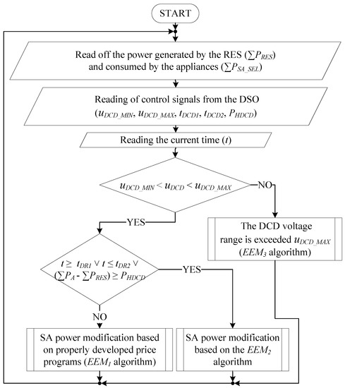
Figure 3.
EEM flow chart.
The complexity of the problem of selecting power settings required the development of an extensive (3) fitness function. Among the set of all power selection options, one combination must be selected that meets criteria for the stated requirements, e.g., reduction of the peak demand phenomenon. The three variants of are intended to respond to the EEM algorithm: user comfort (), requirements set by the DCD () and the situation of exceeding the voltage in the DCD. Equations (4)–(6) make it possible to determine the demand for energy supply in a given DCD. Equation (7), as a component of Equation (3), gives the opportunity to obtain results that, in terms of energy costs and user comfort, will be the most appropriate choice. In case (8), the greatest emphasis in selecting the power settings will be placed on the solutions that will be the best choice for a DCD. In this case, energy costs are a secondary criterion when the most important factor is to keep the energy system in balance, e.g., during environmental phenomena that would contribute to the damaging of the power grid infrastructure.
In , three variants of the implementation of the EEM algorithm for DCDs were taken into account (3).
The first variant () concerns a situation where the task of the EEM algorithm is to ensure the comfort of users by, inter alia, controlling SAs so that the costs for the energy used are as low as possible. For this purpose, the value of is determined from Equation (7). is the current value of power demand for its supply, calculated by , based on selected values of appliance power.
The second variant (3) applies to () and takes into account the need to take action to respond to a crisis situation, e.g., a peak demand phenomenon [21] or damage to the power grid infrastructure. This variant takes into account from Equation (8). is the maximum sum of power of all enabled consumers after the reduction process by , determined individually by the energy consumer. is for the variant which, due to a purpose of use other than , requires the adjustment of Formula (7) of SA power reduction over a specified period of time (from to ) to a value at least equal to .
The third variant (3) takes into account situation (1) when the DCD voltage range is exceeded . In this case, the EEM algorithm based on (2) will select values for all SAs to ensure condition (9).
The EEM algorithm performs its activities in an endless loop. This approach is required due to the dynamics of phenomena occurring over time in Electric Power Systems. Each change requires decisions to be made to ensure a balance between acting for the benefit of DCDs and the comfort of users.
3. Simulation Research
Simulation research for the EEM algorithm was performed in Java in the Eclipse IDE [22]. The implementation of the EEM algorithm in Java required the development of dedicated classes. Among others, the and classes were implemented for the EEM algorithm itself and for storing the required data. Additionally, the , and classes, which are extensions to the class, were implemented. The class introduces the ability to define one of the three available priorities.
The dataset for RESs that was used for simulation research is shown in Figure 4. The data presented in Figure 4 illustrate the situation of the largest generation of energy by a PV source at noon. The collection of such data was done to approximate a typical situation when energy from RESs is available during a selected period of time, so that its excess adversely affects the National Power Systems (NPS).
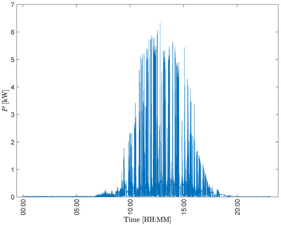
Figure 4.
Sample data from a photovoltaic installation.
In earlier studies, research was conducted for one household [8,23]. The next part of the article presents the results of simulation research for an example of 1000 households. In each of the households, the possibility of using fifteen different SAs was assumed. The operating time profiles and the energy consumed by individual SAs at that time are presented in Figure 5.
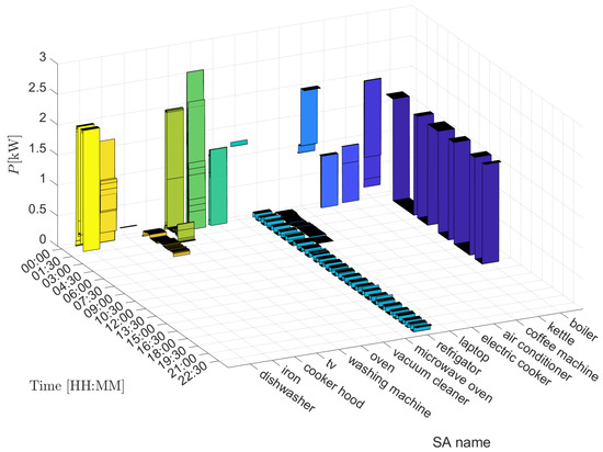
Figure 5.
Profiles of SAs.
Figure 5 shows short profiles of SAs, from half an hour to all-day-long in duration. An example of a short profile is, e.g., the activity of ironing or boiling water in kettles. The operation of the refrigerator, which is switched on periodically throughout the day, can be considered a long profile. In the Figure 5 you can also see energy levels ranging from a few Watts to as much as 3 kW (oven).
The source of data sets defining individual profiles was the recording of measurement data using energy loggers. Data was recorded on exemplary devices that were intended to be general in nature. Particular characteristics were determined on the basis of values obtained from several days of operation of individual devices. The profiles were determined for the purpose of conducting simulation tests, which will be presented later in the article.
Table 1 lists the values of other parameters required for the correct operation of the EEM algorithm.

Table 1.
Definition of other parameters for SAs.
The values of were adopted in such a way as to approximate the typical behavior of users and their needs. The parameter specifies the probability of a given SA occurrence and its launch within a specified time in the range. In order to differentiate individual households, a random selection was used with a given probability of the time when individual SAs are launched. For this purpose, a pseudo-random number generator with a Gaussian distribution, with mean and standard deviation , was used. The value of the time when the SA could be run most often is shown as . On the other hand, the statistical range from when to when a given SA could be run was marked with the following time intervals: from to . Due to the range of SA startup possibilities, it is assumed for all SAs that there will be no shifting during SA startup time ( 0).
Figure 6 shows a histogram for an example of 10,000 times when SA data could be run. In this case, it is assumed that will correspond to 1:45 p.m., when SAs are most likely to be run. The period for contingent activation of SAs was set to the following time range: 12:30 and 15:00.
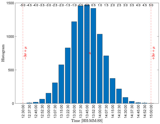
Figure 6.
Histogram of the distribution of times for the interval from 12:30 to 15:00.
Using the rule [24,25,26], a distribution of time values was obtained with a probability of 99.7% falling within the time intervals. It was anticipated that SAs would be launched from 12:30 to 15:00.
In order to verify the correctness of the Java implementation of the activation algorithm of different SAs, the Probability Density Function (PDF) was determined from Formula (10) and the estimator PDF (11) [24,25,26,27]
where S—the number of results in a given range, N—number of results, W—, , and .
In Figure 7, as a result of the statement and , it can be confirmed that the randomly selected values of startup times of a given SA accumulate around 13:45 in the range (from 12:30 to 15:00).
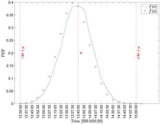
Figure 7.
PDF and estimator PDF for the interval from 12:30 to 15:00.
The verification for starting individual SAs was repeated for a different time range. Again, it was assumed that would correspond to 13:45. The range was changed this time. The time range during which SAs could be run was reduced. The range is from 12: 30 to 14:00. Figure 8 shows a histogram of the times obtained when SAs could be run.
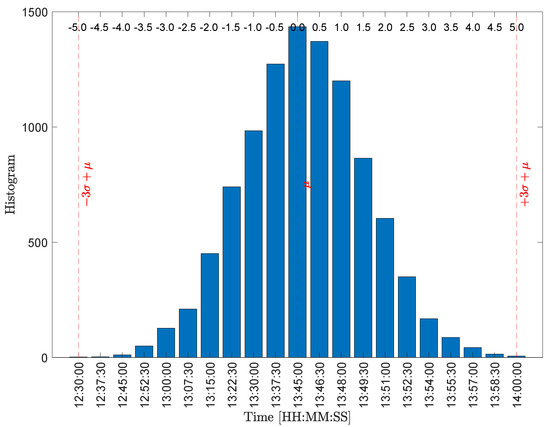
Figure 8.
Histogram of the distribution of times for the interval from 12:30 to 14:00.
Based on the results shown in the histogram (Figure 8), it is unequivocally confirmed that the right-hand range was changed when SAs could be run. As before, the correctness of the obtained results was verified on the basis of the PDF analysis (10) and the PDF estimator (11). The results are presented in Figure 9.
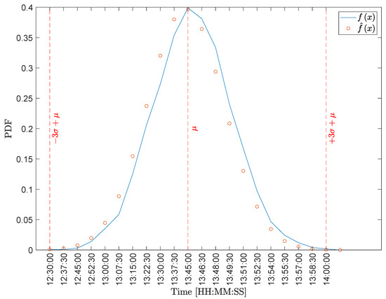
Figure 9.
PDF and estimator PDF for the interval from 12:30 to 14:00.
By conducting an analysis of and from Figure 9, it can be stated that the narrowing of the ranges (on the right) did not adversely affect the randomized values of the activation times of a given SA. SAs are usually run at 13:45 in the range from 12:30 until this time 14:00.
The developed solution of differentiating the times when a given SA would be activated is important in reflecting the behavior in static households for which the EEM algorithm will be used. For example, Figure 10 shows a diagram of the schedule of air conditioners in 1000 households.
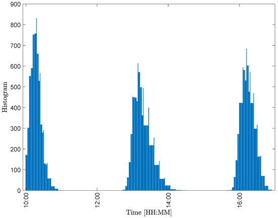
Figure 10.
Air conditioner usage schedule.
The differentiation of start-up times for air conditioners (Figure 10) gives an opportunity to approximate the behavior in typical statistical households. In this case, the data analysis approximates the pattern of behavior of users who, due to e.g., temperature, will statistically want to use air conditioning in similar time ranges. A complete summary of the SA usage pattern in the assumed simulation result is presented in Figure 11.
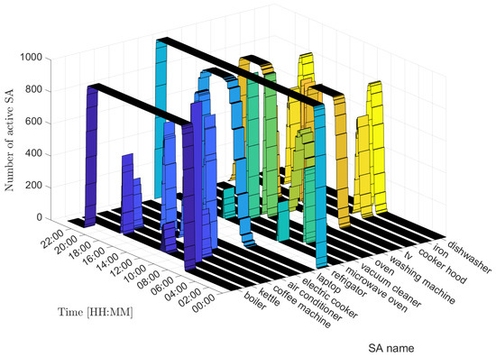
Figure 11.
SA usage schedule.
In the adopted schedule (Figure 11) assumptions were made to approximate the behavior in typical households. It is noticeable that household refrigerators are used all day long. There are also patterns resulting from the desire to use hot water from the boiler. Activities related to daily tasks, such as cooking, cleaning, etc., were also introduced. Based on the adopted schedule (Figure 11), simulation research was carried out. The test results are presented in Figure 12.
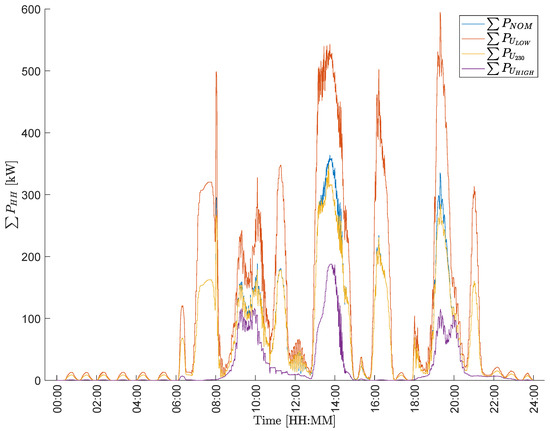
Figure 12.
Energy consumption levels for different voltage ranges.
Figure 12 summarizes the total value of power consumed by 1000 households during one day () for four different variants. The first variant () concerns the situation when the EEM algorithm is not used, so the power values of individual SAs were not modified. The next three variants concern the use of the EEM algorithm when the fitness function (3) is used. The values marked with refer to the situation when the EEM algorithm would increase the load in the DCD network due to the excessively low voltage level . Similarly, the EEM algorithm reduced the load in the network due to the excessively high value of . In the case , the task of the EEM algorithm was to take into account the adjustment to the power generated from RESs (Figure 4). The use of the EEM algorithm resulted in a balance between acting for the benefit of DCDs and the comfort of users. When analyzing the data presented in the Figure 11, the value of is adjusted based on the possibilities specified in .
The EEM algorithm modified the power settings of the SAs only when it was possible. The priorities and the possibility of modifying the power settings of individual SAs are taken into account. The biggest changes in power settings were made between 12:30 and 14:30. Additionally, in Figure 12, changes of power settings are visible from 18:30 to 20:15. Each modification of the power settings of SAs by the EEM algorithm has a direct impact on the total power consumed in the test households (). Noticeable changes in energy consumption in households () are the result of activities that are performed statistically. In most cases, it will be activities related to cooking or cleaning. Using an air conditioner also affects energy consumption. These activities are mainly the most energy-intensive. The case marked as sum230 is not without significance for the user’s comfort and expenses related to the purchase of energy. In this case, the availability of energy from RESs shapes how SAs are used. In such cases, devices such as boilers are activated. This is an example of storing the results of an electrical device.
4. SA Functionality and User Behavior
SA devices should be characterized by the possibility of a flexible switching-on moment activated by a given control signal, e.g., from a DCD or another signal that triggers their operation. In order to provide energy management services in the power grid, SAs should be able to set parameters such as: priority of action, time period during which it can be remotely activated and, if there is such a possibility, operating power. Devices that can be freely turned-on or turned-off are heating/cooling devices. In these cases, it may be possible to turn the device on/off at any point in time, as well as to set the operating power. These devices include fans, air conditioners, electric heaters, boilers, etc. This group of devices also includes all kinds of electric chargers, e.g., electric cars, other electric vehicles, and other battery-powered devices. ESSs should also be included in this group of SAs. They can be charged when there is energy production from RESs. When there is no RES energy production, it should be possible to regulate the charging time and current so as to minimize the impact on power system loading, of course taking into account the comfort of use. On the other hand, ESSs can be discharged at a time of increased demand for electricity by loads, when there is no energy from the power grid (power reduction on demand) [15].
Another group of SAs are those devices that operate continuously but can be deactivated for a short time without detriment to the user’s comfort. These are devices such as a refrigerator or a food freezer. Their operation (on/off) depends on the temperature change set on the thermostat. Due to the large time constant of temperature changes, it is possible to temporarily turn off the devices without significant increases in temperature inside them, which may result in defrosting or spoiling the food [28]. Devices from this group will be used to control the load reduction rather than to increase the load on the power line.
The third group of SAs will be devices whose operation cannot be interrupted after they are turned on due to interference with and poor results of the function performed. This group includes appliances such as dishwashers, electric cookers, washing machines, electric dryers, etc. Disabling them may result in poor quality of washing/dish-washing/cooking etc. Often, interruption of the set operation scenario may result in higher electricity consumption after lowering the operating parameters such as temperature of washing/drying/cooking etc.
A separate group of SAs are devices that are used sporadically or depending on need. These are devices such as irons, hair dryers, electric kettles, coffee makers, etc. Their functionality should be set with a high priority for action, without the possibility of deactivating them. Nevertheless, devices of this type can give information about the state of the power system through some indicator or information on the operator panel. The functionality of individual SAs is summarized in Table 2.
Table 2.
Defining functionality for groups of devices.
In addition to the availability of smart home devices with the possibility of flexible control, in order to be able to effectively manage the electricity consumed in the home, the behavior and habits of electricity users should also be changed [29]. SA users should set their operation to when there is a need to increase the load on the power line, unless it is related to a drastic reduction in their operating comfort. Whenever it is possible, the settings of washing machines and dishwashers should be programmed for the period when the local production from renewable energy sources is at a high level. Similarly, you can change your eating habits for dinner. Often, these meals are prepared after people return home from work. Nevertheless, some of the meals can be remotely set to cook/bake. Then, after people come home from work, the dinner may be already cooked or partially prepared. These activities will require users to be particularly careful in setting up the devices for operation.
Furthermore, some battery-powered devices can be connected and set to charge during energy generation from RESs. The group of such devices includes: home laptops, tablets, portable vacuum cleaners, etc. Electric vehicles should be charged at night, except for the evening peak load of the system. The exception will be when the user defines that he needs the availability of a charged electric vehicle at a designated time. Another change in the habits of electricity users is, for example, ironing clothes, which can be moved to a day when the user is not at work. Of course, this behavior makes sense if there will be energy generation from PV systems on that day. Ironing clothes before going to work increases the morning peak load on the power line.
It is not possible, in a short chapter, to indicate all the functionalities of SAs and changes in the behavior of electricity users. Nevertheless, the description indicates that the use of electricity in the future will involve the intelligent use of home appliances, especially when there is a shortage of power in the electricity system during peak demand and at night. High energy generation from PV systems during the day will imply the problem of excess energy in the system, which must either be stored (expensive solution) or consumed (change in energy use).
5. Experimental Results
Performing full-scale research on a network with available SAs is currently not feasible. Therefore, the article presents simplified results of experimental tests with simulation of SA load changes. The proposed EEM algorithm was implemented in the Programmable AC Load 3091LD [30], while the measurements were made using the HIOKI PW3337 Power Meter [31] (Figure 13). These changes were then scaled and applied to the grid load variability profile and the distributed generation profile from PV installations.
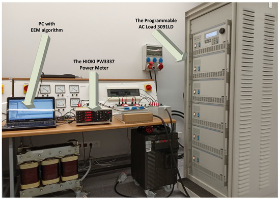
Figure 13.
Photo of the laboratory experimental setup.
Experimental studies were conducted on a group of appliances limited to three SAs, which included a washing machine, an electric boiler and an electric cooker. With the use of the approach proposed in the article, a random load distribution was generated with the use of the indicated SAs.
Each new activation of the algorithm enables the generation of other load data resulting from the probability distribution. The research assumed that for each assay, 100 items of the indicated SM are attached, with an assumed distribution. The proposed experimental verification assumes that all 100 devices will always be in operation in the current study. An example of the variability of a SA switching on based on a washing machine is shown in Figure 14. The top of Figure 14 shows the load distribution for the operation of 1, 2, 5 and 10 washing machines, respectively, while at the bottom of Figure 14, the load distribution for 50, 75 and 100 washing machines is shown. In further studies, a load profile for 100 washing machines was adopted. In addition, similar load distributions were generated for 100 water-heating electric boilers as well as 100 electric cookers.
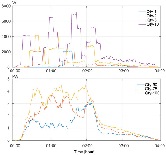
Figure 14.
Load profile for different number of washing machines.
Figure 15 shows an example of the transformer station load profile and the generation of 500 kWp PV installations. Generation values are averaged over 15 min intervals (magenta line at the top of Figure 15). These are the values for a solar day with good PV energy generation. The typical load profile of the power grid is shown with the blue line at the top of Figure 15. The morning and evening grid load peaks are visible. In the hours from about 8:00 to about 15:00, a decrease in the load is visible. At the same time, during these hours, the largest generation profile for PV installations is observed.
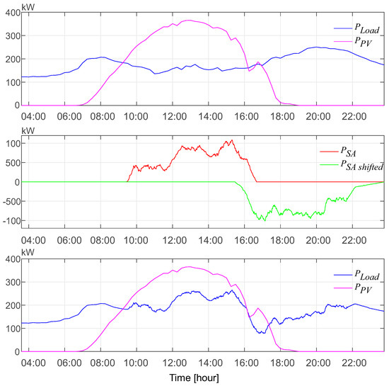
Figure 15.
Experimental results: (top) load profile and generation profile of PV installations; (middle) the power consumed by the SA devices as a result of the proposed EEM algorithm, and an exemplary power profile shifted from the evening hours as a result of not switching on the SA; (bottom) load profile after applying the proposed EEM algorithm and PV installation generation profile.
The task of the algorithm was to shift the load for 100 SAs (washing machine, electric cooker, electric boiler) from evening hours to hours with the highest PV energy generation. The switching-on of the appropriate SAs took place depending on their suitability for the user. The initiation of switching on a selected group of devices and the period of their operation were defined in the tests. Throughout the period of operation of a given group of devices, they were switched on with a given probability distribution. The switching-on of other devices resulted in an increase in the instantaneous load power. Summing up the power consumed in a given period, the energy consumed by a given group of devices was calculated. Then, the power consumed by the given SA group was subtracted from the evening load profile. The power profile that was subtracted was identical to the SA load power profile. The timing of the evening hours during which the load power was shifted was also defined in the proposed test. The data from the performed test are summarized in Table 3. The washing machines were the first to start, as their operation does not have to be coordinated with the user. The wash cycle can start and end at any time of the day. Therefore, the operation of the washing machines was activated at the beginning of the day when there was a large generation of energy from the PV plant. The power consumed by the washing machines was shifted from the evening hours around 19:50 to 23:40. Other devices that were switched on are electric boilers for heating domestic hot water. Due to the good accumulation of heat energy, the heating of the water may be a little earlier than the return of people from work/school. They were turned on from around 11:30 to 14:30. The corresponding power needed to heat the water was shifted from the afternoon hours of 17:40 to 20:40. The last group of devices are electric cookers for preparing dinner. Usually, dinner is prepared after the residents return home from 15:00 to 17:00. If there is a possibility of cooking/baking some dishes, this activity can be performed earlier without the participation of people. The inclusion of smart electric cookers in our research was initiated from 13:40 to 16:40. The power needed to prepare dinner was shifted from the afternoon hours 15:30–18:30. The red color in the middle part of Figure 15 shows the power of devices connected by the proposed EEM algorithm, while the green color shows one of the possible reductions of the peak load. The lower diagram in Figure 15 shows the load profile taking into account the EEM algorithm. There was an increase in load during higher generation from PV and a reduction in power for the evening peak.
Table 3.
Selected SA operating times and energy.
Figure 16 compares the load profile with and without the EEM algorithm. Additionally, at the bottom of Figure 16, the surplus of energy production from PV generation, which should be stored or sent to other loads, is presented. Without the proposed algorithm, the unused energy is exactly 1,039,892 Wh (around 1 MWh), and with the EEM algorithm, it is 648,042 Wh (around 0.65 MWh). The use of the proposed algorithm increased the consumption of electricity during the high output from PV installations and at the same time allowed for a reduction in the evening load on the line. Surplus energy produced from PV sources should be sent to other consumers or stored in ESSs. In the proposed algorithm and the analyzed test, a reduction of the volume of energy to be transmitted or stored by 391,850 Wh was obtained.
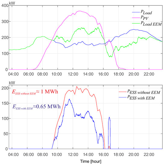
Figure 16.
Experimental results: (top) load profile comparison with and without EEM algorithm; (bottom) comparison of unused energy from PV installation.
6. Conclusions
The use of RESs and temporary load changes (e.g., as a result of the peak demand phenomenon) in Smart Grid (SG) networks require the use of energy management algorithms. The lack of such algorithms would in the worst case result in unstable operation or damage to the electric power system. This article proposes the use of the EEM algorithm for energy management in a hierarchical control system with DCDs. We added the use of the MQTT protocol to our considerations. Such an approach would effectively enable data collection from DCDs. We proposed to use external and internal MQTT brokers to publish data. The data are published with messages that are organized into topics. The topics can contain plain text information. Structures in JavaScript Object Notation (JSON) format can be stored in the text. This format is independent of the specific programming language. This gives the possibility of scalability of the implemented system with new functionalities that would result from the addition of additional IoT devices.
Earlier works [8] considered the use of the EEM algorithm in a single household. Here, the application of the EEM algorithm in 1000 households during simulation studies was outlined. In order to verify the correct operation of the EEM algorithm, test data were developed from the example of a photovoltaic installation (Figure 4). The load profiles of SA devices, which were used in the energy management process, were also developed (Figure 5). Simulation research was carried out with additional assumptions about the priorities for the use of SAs . Differentiation in the use of individual SAs was also obtained on the basis of their parameter specificities and the probability of a given SA occurrence () launched within a specified time in the range. The correctness of a SA’s usability being differentiated from others was confirmed by the determination of the PDF (10) and the estimator PDF (11).
On the basis of the simulation results, it was determined how SAs are used in the exemplary households (Figure 11). The simulation results are presented in Figure 12. In this case, the results of the EEM algorithm for four scenarios are compared. The individual variants reflect the situation where the EEM algorithm is not used, the EEM algorithm is used to increase/decrease the load in the DCD network, or it is used to produce a balance between acting for the benefit of DCDs and the comfort of users.
Experimental studies were carried out for the simplified case with the use of three SAs—a washing machine, an electric boiler and an electric cooker. The algorithm was implemented on an appropriate scale with an adjustable AC load. Then, the obtained results, after scaling, were added/subtracted to/from the previously measured load profile and compared with the generation profile of the PV installation. The obtained results show that by using the proposed EEM algorithm, with the use of SAs, it is possible to change the load profile of the power grid. The evening peak load on the line was reduced and the use of energy produced from the PV installation increased. About 0.35 MWh of energy was shifted using these three types of SA (Figure 16). This means that much less energy from RESs needs to be stored in very expensive ESSs, or that such a volume of energy should be sent to other loads. However, such activities will only be possible if the SAs have the functionality described briefly in Section 4. Additionally, such changes will be related to the change of habits of electricity users. They will have to consciously set the operation of their home appliances to operate at times of high generation coming from renewable energy, i.e., at times when there is a large supply of energy in the grid. They will also have to avoid using their electrical devices (unless there is specific need) in times of heavy load on the grid, when the energy supply in the grid is too small.
At the present stage of research, the biggest limitation for the EEM algorithm is the lack of mass use of SAs in all households. Additionally, data privacy may be an important issue. In this case, it may be about issues related to a lack of will to provide data on activities and tasks carried out by members of society. A solution to this problem may be price incentives encouraging the exchange and sharing of data from new smart devices (SAs).
In our further plans, we intend to design and implement selected types of SAs. Original versions of SAs would be created. Additionally, we plan to implement a prototype of a complete, universal SG network system with SAs. The scope of this work would be the analysis and verification of the EEM algorithm for the IoT concept in electronic device systems. These devices could automatically communicate and exchange data over the network without human intervention. We are also interested in studying the use of energy storage and their inclusion in the EEM algorithm.
Author Contributions
Conceptualization, P.P., P.S. and K.P.; methodology, P.P., P.S., K.P., K.T., M.K. and I.K.; software, P.P.; validation, P.P. and P.S.; formal analysis, P.P. and P.S.; investigation, P.P. and P.S.; resources, P.P. and P.S.; data curation, P.P. and P.S.; writing—original draft preparation, P.P., P.S. and K.P.; writing—review and editing, P.P., P.S. and K.P.; visualization, P.P., P.S., K.P., K.T., M.K. and I.K.; supervision, P.P.; project administration, P.P.; funding acquisition, K.P. All authors have read and agreed to the published version of the manuscript.
Funding
This work was partially funded by the European Union within the European Regional Development Fund (ERDF), in the context of the INTERREG V A BB-PL Programme. Part of this work was carried out as part of the INTERREG Project on “Smart Grid Platform for research on energy management”, project number 85024423 as well as part of the H2020 ebalance plus project (grant number 864283).
Institutional Review Board Statement
Not applicable.
Informed Consent Statement
Not applicable.
Data Availability Statement
Data sharing not applicable.
Conflicts of Interest
The authors declare no conflict of interest.
Abbreviations
The following abbreviations are used in this manuscript:
| DCD | Distributed Control Devices |
| DER | Distributed Energy Resources |
| DR | Demand Response |
| DSO | Distribution System Operator |
| EEM | Elastic Energy Management |
| ESS | Energy Storage Systems |
| GRASP | Greedy Randomized Adaptive Search Procedure |
| IoT | Internet of Things |
| JSON | JavaScript Object Notation |
| MQTT | Message Queue Telemetry Transport |
| NPS | National Power Systems |
| Probability Density Function | |
| PV | Photovoltaic Panels |
| RED II | Renewable Energy Directive |
| RES | Renewable Energy Sources |
| SA | Smart Appliance |
| SG | Smart Grid |
| sum of power consumed in test households during one day | |
| sum of power consumed when the EEM algorithm was to take into account the adjustment to the power generated from RESs | |
| sum of power consumed when the EEM algorithm would decrease the load in the DCD network | |
| sum of power consumed when the EEM algorithm would increase the load in the DCD network | |
| The Probability Density Function (PDF) | |
| The estimator Probability Density Function (PDF) | |
| Component part of the fitness function () aimed at determining the influence of DCD on the choice of power settings | |
| The fitness function | |
| Component part of the fitness function () aimed at determining the influence of RESs on the choice of power settings |
| Component part of the fitness function () aimed at determining the influence of SAs on the choice of power settings | |
| P | A list of other power values for which a given SA could change depending on its working conditions |
| The probability of a given SA occurrence and its launch within a specified time | |
| The nominal power with which the given SA works | |
| SA priority | |
| The time delay property of the given SA startup | |
| DCD voltage | |
| Component part of the fitness function () aimed at taking into account the user’s comfort | |
| Component part of the fitness function () aimed at taking into account the DCD requirements |
References
- European Commission (EC). The European Green Deal, COM(2019) 640. 2019. Available online: https://ec.europa.eu/info/sites/info/files/european-green-deal-communication_en.pdf (accessed on 5 April 2022).
- Directive (EU) 2018/2001 of the European Parliament and of the Council of 11 December 2018 on the Promotion of the Use of Energy from Renewable Sources (Text with EEA Relevance). Available online: http://data.europa.eu/eli/dir/2018/2001/oj (accessed on 5 April 2022).
- Iweh, C.D.; Gyamfi, S.; Tanyi, E.; Effah-Donyina, E. Distributed Generation and Renewable Energy Integration into the Grid: Prerequisites, Push Factors, Practical Options, Issues and Merits. Energies 2021, 14, 5375. [Google Scholar] [CrossRef]
- Naddeo, V.; Korshin, G. Water, energy and waste: The great European deal for the environment. Sci. Total Environ. 2021, 764, 142911. [Google Scholar] [CrossRef] [PubMed]
- Masebinu, S.O.; Akinlabi, E.T.; Muzenda, E.; Aboyade, A.O. Techno-economic analysis of grid-tied energy storage. Int. J. Environ. Sci. Technol. 2018, 15, 231–242. [Google Scholar] [CrossRef]
- Jannesar, M.R.; Sedighi, A.; Savaghebi, M.; Guerrero, J.M. Optimal placement, sizing, and daily charge/discharge of battery energy storage in low voltage distribution network with high photovoltaic penetration. Appl. Energy 2018, 226, 957–966. [Google Scholar] [CrossRef] [Green Version]
- Jabir, H.J.; Teh, J.; Ishak, D.; Abunima, H. Impacts of Demand-Side Management on Electrical Power Systems: A Review. Energies 2018, 11, 1050. [Google Scholar] [CrossRef] [Green Version]
- Powroźnik, P.; Szcześniak, P.; Piotrowski, K. Elastic Energy Management Algorithm Using IoT Technology for Devices with Smart Appliance Functionality for Applications in Smart-Grid. Energies 2022, 15, 109. [Google Scholar] [CrossRef]
- Zhang, F.; Hu, X.; Langari, R.; Wang, L.; Cui, Y.; Pang, H. Adaptive energy management in automated hybrid electric vehicles with flexible torque request. Energy 2021, 214, 118873. [Google Scholar] [CrossRef]
- Jindal, A.; Bhambhu, B.S.; Singh, M.; Kumar, N.; Naik, K. A Heuristic-Based Appliance Scheduling Scheme for Smart Homes. IEEE Trans. Ind. Inform. 2020, 16, 3242–3255. [Google Scholar] [CrossRef] [Green Version]
- Fotopoulou, M.C.; Drosatos, P.; Petridis, S.; Rakopoulos, D.; Stergiopoulos, F.; Nikolopoulos, N. Model Predictive Control for the Energy Management in a District of Buildings Equipped with Building Integrated Photovoltaic Systems and Batteries. Energies 2021, 14, 3369. [Google Scholar] [CrossRef]
- Ouramdane, O.; Elbouchikhi, E.; Amirat, Y.; Le Gall, F.; Sedgh Gooya, E. Home Energy Management Considering Renewable Resources, Energy Storage, and an Electric Vehicle as a Backup. Energies 2022, 15, 2830. [Google Scholar] [CrossRef]
- Shewale, A.; Mokhade, A.; Funde, N.; Bokde, N.D. A Survey of Efficient Demand-Side Management Techniques for the Residential Appliance Scheduling Problem in Smart Homes. Energies 2022, 15, 2863. [Google Scholar] [CrossRef]
- Stanelytė, D.; Radziukynas, V. Analysis of Voltage and Reactive Power Algorithms in Low Voltage Networks. Energies 2022, 15, 1843. [Google Scholar] [CrossRef]
- Smoleński, R.; Szcześniak, P.; Dróżdż, W.; Kasperski, L. Advanced metering infrastructure and energy storage for location and mitigation of power quality disturbances in the utility grid with high penetration of renewables. Renew. Sustain. Energy Rev. 2022, 157, 111988. [Google Scholar] [CrossRef]
- AWS IoT Core Features. Available online: https://aws.amazon.com/iot/ (accessed on 2 May 2022).
- Google Cloud IoT. Available online: https://cloud.google.com/solutions/iot (accessed on 2 May 2022).
- IBM Cloud IoT. Available online: https://www.ibm.com/cloud/internet-of-things (accessed on 2 May 2022).
- Microsoft Azure IoT. Available online: https://azure.microsoft.com/en-us/overview/iot/ (accessed on 2 May 2022).
- Oracle IoT Cloud Service. Available online: https://www.oracle.com/cloud/ (accessed on 2 May 2022).
- Delberis, A.L.; Andrés, M.C.G.; Érica, T.; Eidy, M.M.B. Peak demand contract for big consumers computed based on the combination of a statistical model and a mixed integer linear programming stochastic optimization model. Electr. Power Syst. Res. 2018, 154, 122–129. [Google Scholar] [CrossRef]
- Eclipse IDE and Web IDEs. Available online: https://www.eclipse.org/ide/ (accessed on 5 April 2022).
- Powroźnik, P.; Szulim, R.; Miczulski, W.; Piotrowski, K. Household Energy Management. Appl. Sci. 2021, 11, 1626. [Google Scholar] [CrossRef]
- Ruzgas, T.; Lukauskas, M.; Čepkauskas, G. Nonparametric Multivariate Density Estimation: Case Study of Cauchy Mixture Model. Mathematics 2021, 9, 2717. [Google Scholar] [CrossRef]
- Brajčić Kurbaša, N.; Gotovac, B.; Kozulić, V.; Gotovac, H. Numerical Algorithms for Estimating Probability Density Function Based on the Maximum Entropy Principle and Fup Basis Functions. Entropy 2021, 23, 1559. [Google Scholar] [CrossRef]
- Ngatchou-Wandji, J.; Ltaifa, M.; Njamen Njomen, D.A.; Shen, J. Nonparametric Estimation of the Density Function of the Distribution of the Noise in CHARN Models. Mathematics 2022, 10, 624. [Google Scholar] [CrossRef]
- Lal-Jadziak, J.; Sienkowski, S. Models of bias of mean square value digital estimator for selected deterministic and random signals. Metrol. Meas. Syst. 2008, 15, 55–67. [Google Scholar]
- Werminski, S.; Jarnut, M.; Benysek, G.; Bojarski, J. Demand side management using DADR automation in the peak load reduction. Renew. Sustain. Energy Rev. 2017, 67, 998–1007. [Google Scholar] [CrossRef]
- Zhai, S.; Wang, Z.; Yan, X.; He, G. Appliance Flexibility Analysis Considering User Behavior in Home Energy Management System Using Smart Plugs. IEEE Trans. Ind. Electron. 2019, 66, 1391–1401. [Google Scholar] [CrossRef]
- AC Load 3091LD. Available online: https://www.powerandtest.com/power/electronic-loads/ac-electronic-load-3091ld (accessed on 5 April 2022).
- Power Meter HIOKI PW3337. Available online: https://www.hioki.com/global/products/power-meters/3phase-ac-dc/id_5929 (accessed on 5 April 2022).
Publisher’s Note: MDPI stays neutral with regard to jurisdictional claims in published maps and institutional affiliations. |
© 2022 by the authors. Licensee MDPI, Basel, Switzerland. This article is an open access article distributed under the terms and conditions of the Creative Commons Attribution (CC BY) license (https://creativecommons.org/licenses/by/4.0/).