Borderline SMOTE Algorithm and Feature Selection-Based Network Anomalies Detection Strategy

Abstract

This paper proposes a novel network anomaly detection framework based on data balance and feature selection. Different from the previous binary classification of network intrusion, the network anomaly detection strategy proposed in this paper solves the problem of multiple classification of network intrusion. Regarding the common data imbalance of a network intrusion detection set, a resampling strategy generated by random sampling and Borderline SMOTE data is developed for data balance. According to the features of the intrusion detection dataset, feature selection is carried out based on information gain rate. Experiments are carried out on three basic machine learning algorithms (K-nearest neighbor algorithm (KNN), decision tree (DT), random forest (RF)), and the optimal feature selection scheme is obtained.

1. Introduction

With the continuous development of information technology (IT) and the wide distribution of intelligent facilities, networks composed of various devices that communicate with each other are everywhere. In a smart power grid, advanced measurement systems (AMI) exchange information and control instructions between users and power grid companies through two-way communication with intelligent measurement equipment and routing equipment to regulate power grid operation and realize power flow calculation, load prediction, load response and other functions [1]. While IT brings the benefits of real-time monitoring of the power grid, IT also leads to AMI’s vulnerability to network attacks [2]. For example, the network attack on the Ukrainian power grid in 2015 led to the serious consequences of a large-scale power outage [3]. As the network security of a cyber physical system (CPS) is of great importance, the network security of AMI has attracted more and more attention [4,5,6]. The purpose of a network attack is to break the integrity, confidentiality and availability of data; thus, as to obtain some benefits. In AMI, there are various methods of network attacks. For example, hackers can access the master station illegally through the intrusion concentrator to tamper and delete data. Conversely, by physically accessing electricity meters, hackers can use cache overflow to obtain the root permission of electricity meters and then implement a distributed Dos attack. For these network attacks, there are two major defense methods: authentication [7,8,9] and intrusion detection [5,10,11]. With the evolution of network attacks, it is important to ensure network security through intrusion detection. The main purpose of this article is to verify that the proposed method can effectively perform feature selection in the presence of multiple features.

2. Literature Review

Intrusion detection technology can be divided into two types: anomaly detection [12] and misuse detection [13]. The main difference between the two is whether the characteristics of network attacks are known. Machine learning-based misuse detection can extract features of network attacks through supervised learning or semi-supervised learning to significantly improve the accuracy of detection [14]. When the characteristics of network attacks are unknown, the normal behavior pattern of the network can be established through machine learning, and the network attacks can be classified by the mismatch between the network behavior under attack and the normal pattern [15]. In [15], due to the fact that the real-time traffic in Internet of Things is too large, it is impossible to label each data in real time, and a semi-supervised deep learning framework is introduced, making use of both labeled and unlabeled traffic sequences during training. With an attention module introduced and the training procedures for each separate part in a gradual strategy, the proposed model shows superiority across different measures and has computational effectiveness. In [16], to avoid the dimension disaster, an improved binary gravitational search algorithm is used to improve a support vector machine for the classification of attacks, and it strikes a balance between detection efficiency and robustness. Compared with machine learning, deep learning is also widely used in network intrusion detection due to its high efficiency in setting layers and extracting effective information from training data [17]. In [18], a convolution neural network is used to extract data features from a large number of network data. Combined with generative adversarial network and fuzzy rough set, an intrusion detection algorithm suitable for different scenarios is established, and it is validated that the proposed intelligent algorithm has higher accuracy.

Drawing on the advantages of deep learning, traditional machine learning algorithms are combined with feature selection and are widely applied in the field of network intrusion detection, such as random forest, support vector machine, K-nearest neighbor, decision tree, etc. [19,20], all of which have achieved good results. Commonly used datasets related to intrusion detection include KDD Cup 99, DARPA 1998, ADFA-LD, CIC-IDS2017, UNSW-NB15, etc. Among them, the CIC-IDS2017 dataset contains a large amount of traffic data and a large number of features for anomaly detection [21]. Compared with other datasets, CIC-IDS2017 has more features and more data, making it easier to verify the effectiveness of the proposed method. Therefore, the following problems may occur when using the traditional machine learning algorithm for the intrusion detection of CIC-IDS2017:

(1)

There are too many features in the dataset. For example, [22] optimized the parameter and weight selection of support vector machine based on a genetic algorithm and combined with feature selection, which improved the intrusion detection rate and reduced the training time of the SVM (support vector machine). However, the dataset used, KDD Cup 99, only had 41 features, while CIC-IDS2017 had 78 features.

(2)

Unbalanced dataset: For example, in [21], an unbalanced dataset is used, resulting in a poor detection effect for a few classes.

(3)

Binary classification problem and multi-classification problem: at present, most studies are focused on abnormal binary classification problems [23,24]; that is, each classifier can only detect one attack mode; and there is little research on the multi-classification of network attacks based on the CIC-IDS dataset [25]. Not only is this a waste of computing resources, it is also hard to identify different types of attacks.

In view of these problems, this paper uses the Borderline SMOTE algorithm to oversample a small amount of data to avoid data imbalance, then puts forward the feature selection method based on information gain rate, and applies three common machine learning algorithms on different feature selection datasets, obtaining the best feature selection and machine learning method. In contrast to [25], we adopt the SMOTE method for the problem of sample imbalance and expand the amount of some data with a small proportion, making the classification model more sensitive to these types of attacks. The second section introduces the relevant knowledge, the third section introduces the proposed network intrusion detection framework and results analysis, and the fourth section is the conclusion.

3. Findings

The algorithm proposed in this paper is based on the CIC-IDS 2017 dataset. Firstly, the Border Line SMOTE algorithm is used to balance the dataset, and then the information gain ratio is used for feature selection to obtain a suitable dataset. Section 3 is the preliminary part, Section 3.1 introduces the dataset, and Section 3.2 introduces the Border Line SMOTE algorithm, which is mainly used for balancing datasets. Section 3.3 introduces the information gain ratio; the calculation of the information gain ratio involves entropy and information gain. Section 3.4 introduces the evaluation metrics of the algorithm.

3.1. Dataset

In this paper, network information attack detection is carried out based on the CIC-IDS2017 dataset. The CIC-IDS dataset is a network intrusion detection dataset designed, collected, and processed by Sharafaldin et al. [26] from The Canadian Security Research Institute in 2017. Compared with NSL-KDD and other popular datasets in the field of network intrusion detection, it has richer and more diverse data categories.

The CIC-IDS dataset collected a total of 2,830,743 network traffic data pieces. Each piece of data has 78 characteristics and contains tag data. The dataset has 15 different labels. The specific labels are BENIGN, DoS Hulk, Port Scan, DDoS, DoS Golden Eye, FTP-Patator, SSH-Patator, DoS slow loris, DoS Slow http test, Bot, Web Attack Brute Force, Web Attack XSS, Infiltration, Web Attack SQL Injection, Heartbleed, Bot, and Web Attack Brute Force. The proportion of each type of data is given in Table 2 of Section 3.1. The features of the dataset are obtained through CIC Flow Meter, including Source IP, Source Port, Destination IP, Destination Port, and Protocol. All extracted features are defined and explained on the CIC Flow Meter webpage (Canadian Institute for Cybersecurity). Table 3 in Section 3.1 lists all the features. Compared with other datasets, this dataset not only has a large amount of data, but also has a large number of features. The results of different feature selection are sensitive. Thus, we use this dataset.

3.2. Borderline SMOTE

Borderline SMOTE is an improved oversampling algorithm based on SMOTE, which uses only a few class samples on the border to combine new samples, thus improving the sample category distribution. Borderline SMOTE samples are divided into three categories: Safe, Danger and Noise. Finally, only a few Danger samples were oversampled. The algorithm steps are as follows:

(1)

For every sample in a few classes $x_i$, compute the nearest m samples from the entire dataset. The number of other categories in the most recent samples m is denoted by $m^{\prime }$.

(2)

Classify the samples $x_i$:

If $m^{\prime }=m$, the surrounding samples of $x_i$ are all samples of different categories, which are denoted as noise data. Such data will have adverse effects on the generation effect; thus, it is considered not to use these samples in the generation.

If $m/2\le m^{\prime }<m$, more than half of the surrounding m samples of $x_i$ are of different categories. Define the boundary sample as Danger.

If $0\le m^{\prime }<m/2$, more than half of the surrounding m samples of $x_i$ are of the same categories, denoted as Safe.

(3)

After the marking, use the SMOTE algorithm to expand the Danger samples. Select $x_i$ in the Danger dataset samples, compute k-nearest neighbor samples of the same kind $x_{zi}$. New samples $x_n$ are randomly synthesized according to the following formula

$$x_n=x_i+\beta (x_{zi}-x_i)$$

where $\beta$ is a random number between 0 and 1.

In addition, have Borderline-SMOTE1 and Borderline-SMOTE2, Borderline-SMOTE1 randomly select a few types of samples in the K-nearest neighbor sample during new SMOTE for Danger (same as SMOTE) and Borderline-SMOTE2 in any samples in the k-nearest neighbor (regardless of sample category). The above algorithm steps are the Borderline-SMOTE1 algorithm.

3.3. Information Gain Ratio

The information gain ratio is a method to achieve feature selection, which is calculated by information gain. Information gain calculates the reduction in entropy or surprise from transforming a dataset in some way. First, we introduce information entropy. Information entropy is a value that measures the stability of the system, which is calculated as

$$Ent(x)=-{\displaystyle \sum _{x\in X}p(x)\log p(x)}$$

The more unstable a system is, or the more uncertain it is that something will happen, the higher its entropy.

Conditional entropy is the entropy of the system for given attribute A

$$Ent(X|A)={\displaystyle \sum _{a\in A}p(a)Ent(X|A=a)}$$

The information gain represents the extent to which the information of attribute A reduces the uncertainty of information of X

$$Gain(X,A)=Ent(X)-Ent(X|A)$$

Since the information gain criterion has a preference for more desirable features, the information gain rate is proposed for feature selection

$$GainRatio(X,A)=\frac{Gain(X,A)}{IV(A)}$$

where

$$IV(A)=-{\displaystyle \sum _{a\in A}p(a|A)\log p(a|A)}$$

IV (intrinsic value) represents a fixed value for an attribute, and $p(a|A)$ represents the proportion of a in A. If there is only one type of data in A, e.g., $p(a|A)=1$, then $IV(A)=0$. As a result, the calculation of information gain rate based on the formula will be wrong. In this case, the information gain rate is 0.

3.4. Metric Performance

For the dichotomous problem, we propose to measure the classification performance based on the precision and recall of the confusion matrix, which can be generalized to the multi-classification problem. Multiple dichotomous confusion matrices can obtain multiple accuracy and recall as shown in the following

Table 1. Metric performance.

Metric	Binary Classification
Confusion Matrix			Predicted Label
			Positive	Negative
	Actual Label	Positive	TP	FN
		Negative	FP	TN
Accuracy	$A=\frac{TP+TN}{TP+FP+FN+TN}$
Recall/True Positive Rate	$R=\frac{TP}{TP+FN}$
	Multi Class Classification
Confusion Matrix			Predicted Label
			Class-1	……	Class-n
	Actual Label	Class-1	$\mathrm{Matrix} C\in R^{n\times n}$
		……
		Class-n
Accuracy	$A=\frac{{\displaystyle \sum _{i=1}^n{C}_{ii}}}{{\displaystyle \sum _{i=1}^n{\displaystyle \sum _{j=1}^n{C}_{ij}}}}$
Recall/True Positive Rate	$R_i=\frac{C_{ii}}{{\displaystyle \sum _{j=1}^n{C}_{ij}}}$$MacroR=\frac{1}{n}{\displaystyle \sum _{i=1}^n{P}_i}$

.

Among the multi-classification problems studied in this paper, the global accuracy rate, macro recall rate, and various recall rates are selected as the result evaluation indexes

4. Discussion

Based on the method proposed in the last chapter, a flow chart of the algorithm is designed to illustrate its execution steps. Figure 1 is the network attack detection framework proposed by us, which is divided into the following four steps:

The input data of resample is the original CIC-IDS 2017 dataset, and the data are resampled to obtain a balanced dataset. For the specific sampling algorithm, see Section 4.1.1.

Taking 70% of the data of the balanced dataset as the training set and 30% of the data as the test set, the information gain rates of different features of the training set data are calculated and sorted, and they are divided into different combinations based on the confidence gain rate. See Section 4.1.2 for details.

Apply the machine learning algorithm to different groups and test them on the test set, and evaluate the results based on the evaluation indicators in Section 3.4 to obtain the optimal feature group sum.

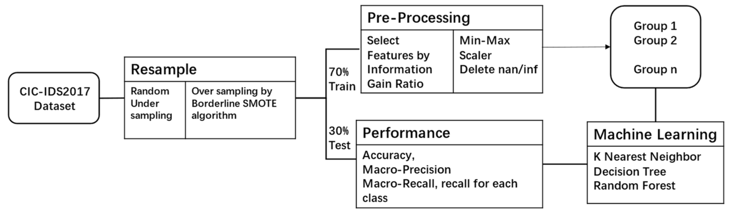
4.1. Data Preprocess

4.1.1. Data Resampling

First, the algorithm requires resampling unbalanced data in the CIC-IDS2017 dataset. There are 14 types of data in the CIC-IDS2017 dataset. The 14 types of data are divided into three categories according to the sample size: L (little), A (a little), and P (plenty). In the original dataset, the number of data with different labels is sorted in descending order, and the results are shown in the following table. Calculate the ratio of the numbers between adjacent labels and obtain (9.8700 1.4491 1.2404 12.4381 1.2972 1.3456 1.0174 1.0540 2.8113 1.2979 2.3113 18.1111 1.7143 1.9091). Therefore, the data are divided into three categories from the difference of more than ten times, which are L (Web Attack SQL, Injection, Heartbleed), P (BENIGN, DoS Hulk, Port Scan, DDoS), and A (others). For the category with a small sample size (L), such as Web Attack SQL Injection, there are only 21 cases of data, which are not considered in the algorithm and can be directly deleted. Random undersampling was used for categories with large sample sizes (p). For categories with a small sample size (A), the Borderline SMOTE algorithm is utilized to increase the sample size.

Table 2. CIC-IDS dataset, resampled dataset, training dataset and test dataset.

Class	CIC-IDS Dataset	Resampled Dataset	Training Dataset	Testing Dataset
BENIGN	2,271,320	20,000	13,973	6027
DoS Hulk	230,124	20,000	13,962	6038
PortScan	158,804	20,000	13,994	6006
DDoS	128,025	20,000	14,161	5839
DoS GoldenEye	10,293	10,293	7221	3072
FTP-Patator	7935	7935	5589	2346
SSH-Patator	5897	5897	4130	1767
DoS slowloris	5796	5796	4046	1750
DoS Slowhttptest	5499	5499	3829	1670
Bot	1956	5000	3447	1553
Web Attack Brute Force	1507	5000	3470	1530
Web Attack XSS	652	5000	3472	1528
Infiltration	36	0	0	0
Web Attack Sql Injection	21	0	0	0
Heartbleed	11	0	0	0
Total	2,827,876	145,420	87,847	37,573

shows the sample size of each dataset after resampling.

The first column of the table records the number of types of data in the CIC-IDS dataset after the NAN, INF, and NULL values are removed. There are 2,830,743 pieces of data in the original CIC-IDS-dataset, and 2,827,876 pieces of valid data after deleting NAN, INF and NULL values. In this case, data sampling is achieved by Random Under Sampler and Borderline SMOTE and 145,420 pieces of data are obtained, 70% of which are taken as the training set while other 30% are treated as the testing set.

4.1.2. Data Preprocessing and Feature Selection

After resampling the data, the balanced dataset is obtained, and the information gain rate of each feature on the balanced dataset is calculated. The results are shown in

Table 3. Feature rank generated by information gain ratio.

No.	ID	Feature Names	IGR
1	69	min_seg_size_forward	0.642905
2	67	Init_Win_bytes_backward	0.568649
3	66	Init_Win_bytes_forward	0.534474
4	11	Bwd Packet Length Min	0.500375
5	5	Total Length of Bwd Packets	0.479726
6	65	Subflow Bwd Bytes	0.479726
7	35	Bwd Header Length	0.477581
8	34	Fwd Header Length	0.46183
9	55	Fwd Header Length.1	0.46183
10	30	Fwd PSH Flags	0.460098
11	44	SYN Flag Count	0.460098
12	39	Max Packet Length	0.444258
13	12	Bwd Packet Length Mean	0.439078
14	54	Avg Bwd Segment Size	0.439078
15	10	Bwd Packet Length Max	0.426576
16	43	FIN Flag Count	0.420984
17	3	Total Backward Packets	0.41914
18	64	Subflow Bwd Packets	0.41914
19	48	URG Flag Count	0.412948
20	0	Destination Port	0.411226
21	2	Total Fwd Packets	0.404084
22	62	Subflow Fwd Packets	0.404084
23	68	act_data_pkt_fwd	0.399244
24	38	Min Packet Length	0.395738
25	7	Fwd Packet Length Min	0.392421
26	6	Fwd Packet Length Max	0.382406
27	4	Total Length of Fwd Packets	0.356587
28	63	Subflow Fwd Bytes	0.356587
29	46	PSH Flag Count	0.34864
30	51	Down/Up Ratio	0.346817
31	13	Bwd Packet Length Std	0.344646
32	52	Average Packet Size	0.338569
33	40	Packet Length Mean	0.335255
34	8	Fwd Packet Length Mean	0.320388
35	53	Avg Fwd Segment Size	0.320388
36	75	Idle Std	0.317702
37	42	Packet Length Variance	0.299398
38	41	Packet Length Std	0.297963
39	9	Fwd Packet Length Std	0.291304
40	76	Idle Max	0.254416
41	23	Fwd IAT Max	0.254233
42	74	Idle Mean	0.252443
43	20	Fwd IAT Total	0.251187
44	21	Fwd IAT Mean	0.24798
45	22	Fwd IAT Std	0.234591
46	77	Idle Min	0.233341
47	17	Flow IAT Std	0.231187
48	25	Bwd IAT Total	0.219028
49	18	Flow IAT Max	0.218065
50	24	Fwd IAT Min	0.215989
51	47	ACK Flag Count	0.21487
52	14	Flow Bytes/s	0.212526
53	28	Bwd IAT Max	0.212366
54	26	Bwd IAT Mean	0.21108
55	29	Bwd IAT Min	0.20972
56	37	Bwd Packets/s	0.208757
57	16	Flow IAT Mean	0.208709
58	71	Active Std	0.206242
59	15	Flow Packets/s	0.203749
60	36	Fwd Packets/s	0.203416
61	1	Flow Duration	0.20025
62	27	Bwd IAT Std	0.20008
63	70	Active Mean	0.196345
64	72	Active Max	0.196185
65	73	Active Min	0.193686
66	45	RST Flag Count	0.177221
67	50	ECE Flag Count	0.177221
68	32	Fwd URG Flags	0.16054
69	49	CWE Flag Count	0.16054
70	19	Flow IAT Min	0.153983
71	31	Bwd PSH Flags	0
72	33	Bwd URG Flags	0
73	56	Fwd Avg Bytes/Bulk	0
74	57	Fwd Avg Packets/Bulk	0
75	58	Fwd Avg Bulk Rate	0
76	59	Bwd Avg Bytes/Bulk	0
77	60	Bwd Avg Packets/Bulk	0
78	61	Bwd Avg Bulk Rate	0

.

Note that the IDs are numbered from 0 to 77. It can be seen from Table 3 that the feature with the maximum information gain rate is min seg_size_forward, and there are eight features with an information gain rate of 0, indicating that these features have only one type in the balanced dataset and therefore have no effect in classification. Different datasets were divided based on different thresholds, and the thresholds were set as 0.5, 0.4, 0.3, 0.2, 0.1 to obtain the feature sets in

Table 4. Selected features by information gain ratio.

Group	Criterion	Number of Selected Feature	Selected Feature
Group 1	>0.5	4	69, 67, 66, 11
Group 2	>0.4	22	69, 67, 66, 11, 5, 65, 35, 55, 34, 30, 44, 39, 12, 54, 10, 43, 64, 3, 48, 0, 62, 2
Group 3	>0.3	36	69, 67, 66, 11, 5, 65, 35, 55, 34, 30, 44, 39, 12, 54, 10, 43, 64, 3, 48, 0, 62, 2 68, 38, 7, 6, 4, 63, 46, 51, 13, 52, 40, 53, 8, 75
Group 4	>0.2	62	69, 67, 66, 11, 5, 65, 35, 55, 34, 30, 44, 39, 12, 54, 10, 43, 64, 3, 48, 0, 62, 2 68, 38, 7, 6, 4, 63, 46, 51, 13, 52, 40, 53, 8, 75, 42, 41, 9, 76, 23, 74, 20, 21, 22, 77, 17, 25, 18, 24, 47, 14, 28, 26, 29, 37, 16, 71, 15, 36, 1, 27
Group 5	>0.1	70	69, 67, 66, 11, 5, 65, 35, 55, 34, 30, 44, 39, 12, 54, 10, 43, 64, 3, 48, 0, 62, 2 68, 38, 7, 6, 4, 63, 46, 51, 13, 52, 40, 53, 8, 75, 42, 41, 9, 76, 23, 74, 20, 21, 22, 77, 17, 25, 18, 24, 47, 14, 28, 26, 29, 37, 16, 71, 15, 36, 1, 27, 70, 72, 73, 45, 50, 32, 49, 19
Group 6	All	78	All Feature

[21]. Six different datasets were constructed based on the following six feature sets to test the results of the algorithm when taking different features.

In addition, the maximum and minimum normalization method is used to normalize the data in the pre-processing stage.

4.2. Evaluation of Models

4.2.1. Model construction and Training Phase

This part mainly lies in training the processed data based on common machine learning algorithms (K-nearest neighbor method, decision tree, random forest).

K-nearest neighbor algorithm:k-nearest neighbor algorithm is a relatively mature and simplest machine learning algorithm, which can be used for basic classification and regression methods. The main idea of the algorithm is that if a sample is most similar to k instances in the feature space (that is, the nearest neighbor in the feature space), then the sample also belongs to the category to which most of the k instances belong. In the classification problem, the new sample is predicted by majority voting according to the classification of its k-nearest neighbor training samples.

Decision tree: Decision tree forms a tree structure model from the training data. The decision-making process of decision tree is to start from the root node. Then, it tests the corresponding characteristic attributes of the item to be classified and selects the output branches according to their values until it reaches the leaf node. Finally, it stores the categories in the leaf node as the decision result. The key of establishing a decision tree is to choose the attribute as the classification basis in the current state. According to different objective functions, there are mainly three algorithms to establish decision trees: ID3 (iterative dichotomiser), C4.5 and CART (classification and regression tree). They take information gain, information gain rate and Gini index mean square deviation as the basis of feature selection, respectively.

Random forest: This method creates a forest in a random way. The random forest algorithm consists of many decision trees, each of which has no correlation. After the establishment of the forest, when new samples enter, each decision tree will make a judgment separately and then give classification results based on a voting method. Random forest is an extended variant of bagging, which further introduces random feature selection in the training process of the decision tree on the basis of constructing a bagging ensemble based on the decision tree learner.

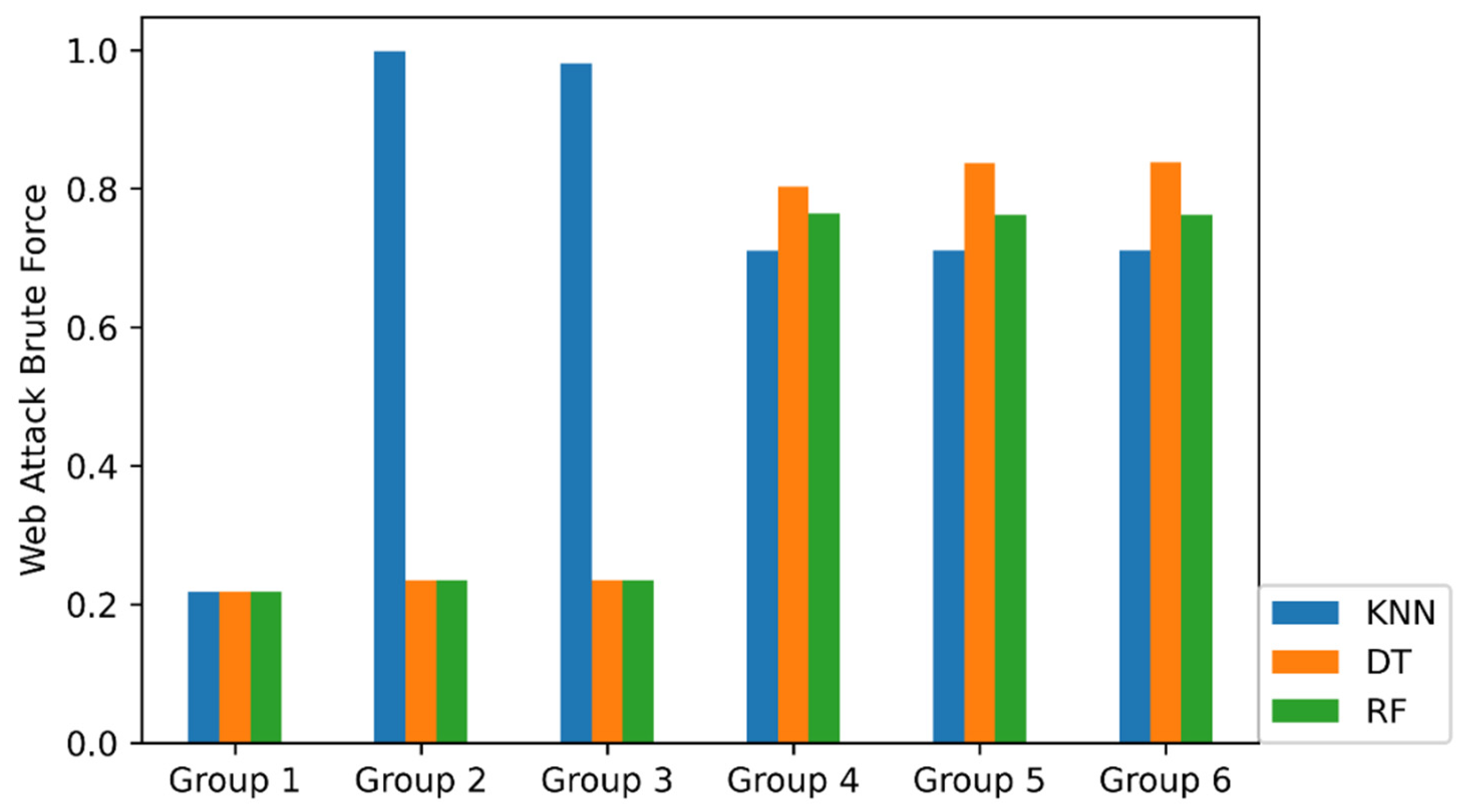
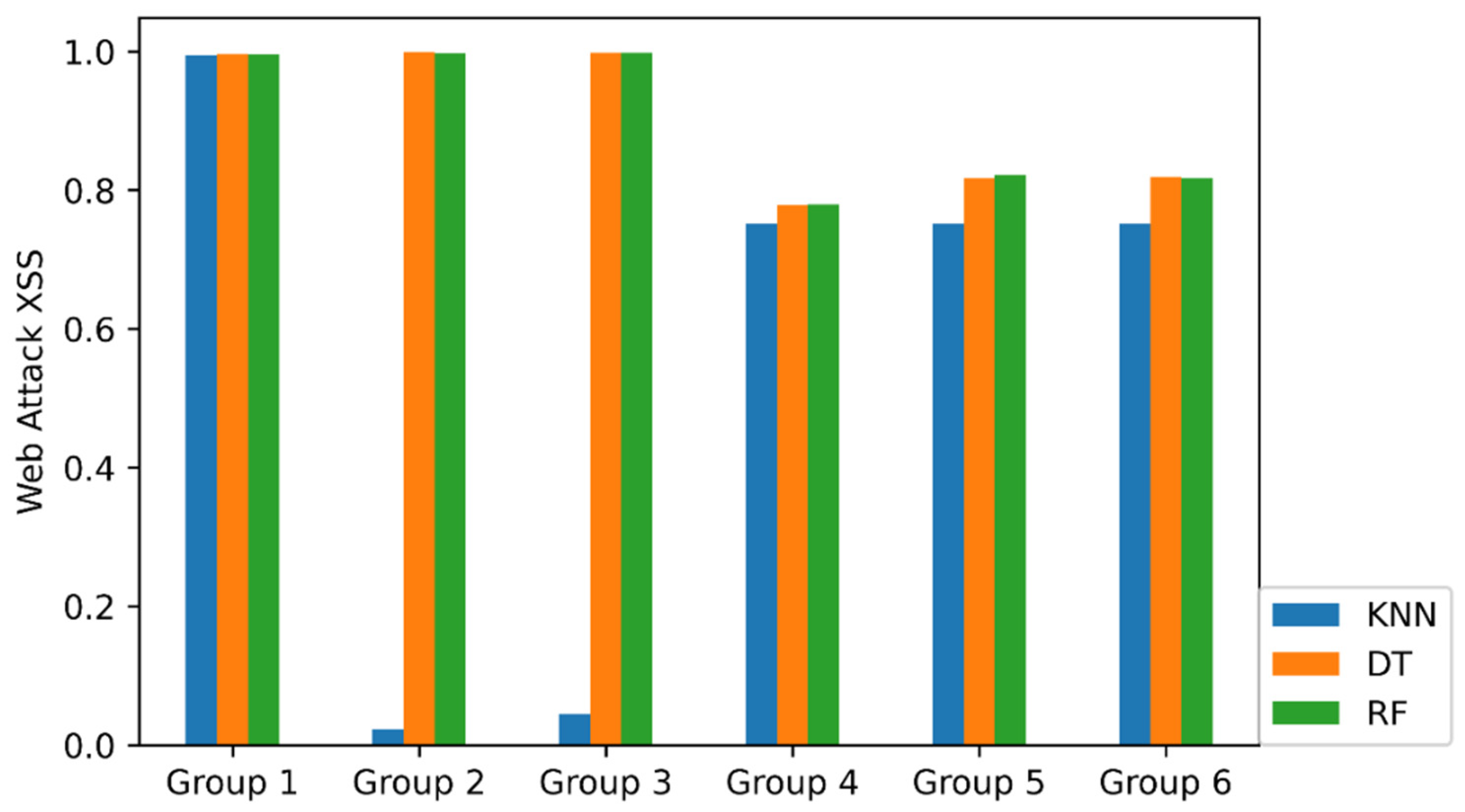
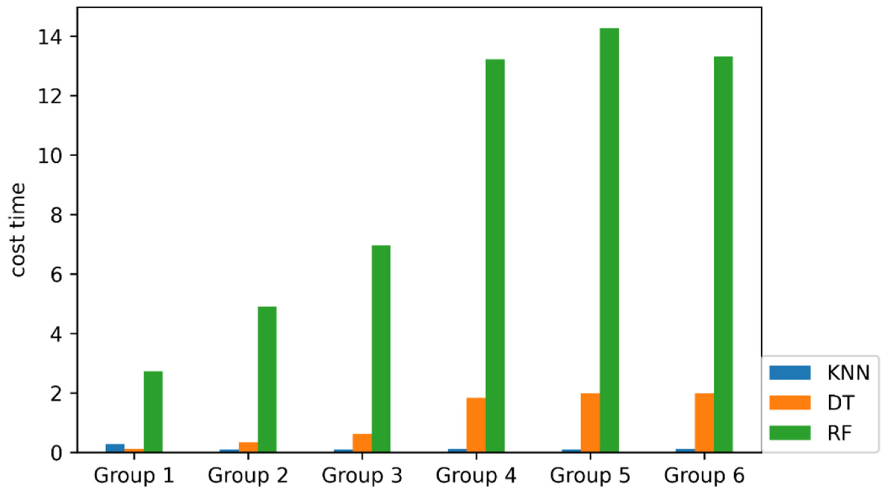
4.2.2. Evaluation of Models

The trained model is tested on the testing dataset based on the evaluation index of Section 4.2.1 to evaluate the algorithm performance. The results are shown in

Table 5. Results.

Group	Method	Accuracy	BENING	Bot	DDoS	DoS Golden Eye	DoS Hulk	DoS Slow http Test
1 (4 features)	KNN	0.8945	0.9497	0.9672	0.9990	0.9993	0.9268	0.1252
	DT	0.9144	0.9537	0.9736	0.9990	0.9993	0.9324	0.5665
	RF	0.9146	0.9539	0.9781	0.9990	0.9993	0.9323	0.5665
2 (22 features)	KNN	0.9523	0.9617	0.9749	0.9955	0.9980	0.9962	0.9880
	DT	0.9666	0.9910	0.9910	0.9981	0.9990	0.9975	0.9886
	RF	0.9672	0.9935	0.9936	0.9986	0.9997	0.9980	0.9868
3 (36 features)	KNN	0.9541	0.9740	0.9871	0.9949	0.9987	0.9925	0.9874
	DT	0.9668	0.9910	0.9929	0.9985	0.9993	0.9974	0.9880
	RF	0.9672	0.9932	0.9923	0.9986	0.9993	0.9980	0.9886
4 (62 features)	KNN	0.9702	0.9655	0.9942	0.9932	0.9987	0.9949	0.9922
	DT	0.9808	0.9939	0.9923	0.9985	0.9980	0.9980	0.9934
	RF	0.9802	0.9934	0.9974	0.9986	0.9993	0.9997	0.9916
5 (70 features)	KNN	0.9704	0.9647	0.9942	0.9926	0.9987	0.9970	0.9922
	DT	0.9840	0.9952	0.9910	0.9990	0.9990	0.9978	0.9928
	RF	0.9818	0.9930	0.9981	0.9983	0.9993	0.9998	0.9922
6 (78 features)	KNN	0.9704	0.9647	0.9942	0.9926	0.9987	0.9970	0.9922
	DT	0.9841	0.9952	0.9910	0.9986	0.9987	0.9978	0.9928
	RF	0.9814	0.9924	0.9974	0.9985	0.9990	0.9997	0.9916
Group	Method	Micro RECALL	DoS Slow Loris	FTP-Patator	Port Scan	SSH-Patator	Web Attack Brute Force	Web Attack XSS
1 (4 features)	KNN	0.8234	0.9029	0.8103	0.9953	0.9932	0.2170	0.9948
	DT	0.8548	0.6309	0.9987	0.9953	0.9943	0.2176	0.9961
	RF	0.8552	0.6309	0.9987	0.9953	0.9943	0.2183	0.9954
2 (22 features)	KNN	0.9104	0.9943	1.0000	0.9983	0.9972	0.9980	0.0223
	DT	0.9326	0.9954	1.0000	0.9988	1.0000	0.2340	0.9980
	RF	0.9330	0.9960	1.0000	0.9992	0.9977	0.2346	0.9980
3 (36 features)	KNN	0.9122	0.9926	1.0000	0.9983	0.9960	0.9804	0.0445
	DT	0.9329	0.9954	1.0000	0.9992	1.0000	0.2353	0.9980
	RF	0.9330	0.9954	1.0000	0.9992	0.9989	0.2346	0.9980
4 (62 features)	KNN	0.9486	0.9920	0.9983	0.9985	0.9943	0.7098	0.7513
	DT	0.9619	0.9920	0.9996	0.9995	1.0000	0.8039	0.7742
	RF	0.9600	0.9960	1.0000	0.9997	0.9966	0.7686	0.7795
5 (70 features)	KNN	0.9487	0.9920	0.9983	0.9985	0.9943	0.7105	0.7513
	DT	0.9681	0.9931	0.9991	0.9998	1.0000	0.8340	0.8161
	RF	0.9637	0.9954	1.0000	0.9995	0.9972	0.7601	0.8318
6 (78 features)	KNN	0.9487	0.9920	0.9983	0.9985	0.9943	0.7105	0.7513
	DT	0.9684	0.9931	0.9991	0.9998	1.0000	0.8353	0.8194
	RF	0.9631	0.9949	1.0000	0.9995	0.9966	0.7627	0.8246

.

5. Conclusions

According to the execution steps shown in Section 4, simulations have been carried out in this part.

Table 5 shows the results of KNN, DT, and RF on six datasets. As can be seen from Group 1’s result, when only four features with the highest information gain rate are selected, the accuracy of the random forest model in the testing dataset can reach 91.46%. DoS Slow HTTP Test and Web Attack Brute Force had low recall under the three algorithms.

Group 2’s results show where the former 22 features whose information gain is greater than 0.4 were taken. At this point, the recall rate of the DoS Slow HTTP test is greater than 98% under all three algorithms, and the result is good, indicating that the reason for the low recall rate of the DoS Slow HTTP test in Group 1 is that the features related to DoS Slow HTTP test are not in Group 1. However, the recall rate of Web Attack Brute Force on the KNN model is 99%, and the recall rate on DT and RF is still low, indicating that KNN is suitable for detecting Web Attack Brute Force. The Web Attack XSS works poorly on KNN and is almost impossible to detect. In addition, the overall accuracy rate and macro recall rate of Group 2 are better than those of Group 1.

Group 3’s result compared with group 2’s, taking the former 36 features, does not greatly improve the results.

Group 4 takes the former 62 features. At this time, the recall rate of Web Attack Brute Force among the three algorithms improved, and the recall rate of Web Attack XSS on KNN also increased from 4% to 75%. However, the recall rate of the other two algorithms decreased from 99% to 77%. The overall accuracy rate and macro recall rate of Group 4 are greatly improved.

Group 5 takes the top 70 features, and Group 6 takes all features into consideration, which shows no significant improvement compared with the results of Group 4.

Figure 2 is the schematic diagram of the overall accuracy of the three algorithms in the six groups. It can be seen that the results of Group 4, Group 5 and Group 6 are basically the same; that is, when the number of features is more than 62, adding features has no effect on the overall accuracy. The main contribution of this paper is to propose an algorithmic framework based on feature selection and data balance, rather than the final machine learning algorithm. From the results, it can be seen that when selecting suitable features, choosing different machine learning algorithms has little effect on the results, such as Group 6 in Figure 2. Even a not-so-advanced machine learning algorithm such as decision tree has a final accuracy rate of over 99%; thus, the algorithm in this paper has application value compared to the state of the art.

Figure 3 and Figure 4 show recall rates of Web Attack Brute Force and Web Attack XSS under different algorithms and feature selection. Web Attack Brute Force chose the KNN algorithm in Group 2 with the highest recall rate. The recall rate of Web Attack XSS decreases with the increase in features.

Figure 5 shows the training time of the three algorithms. It can be seen that as an ensemble-learning algorithm, the training time of random forest is much longer than that of the decision tree and K-nearest neighbor algorithms. There is little difference in the training time between KNN and DT when the number of data features is low. When the data features increase, the training time of decision tree is also much longer than that of KNN. The difference in training time is determined by the algorithm. Both KNN and DT are single models, while RF is an ensemble algorithm composed of multiple RTs; thus, the training time is more. More specifically, the time to train the model is related to the time complexity of the algorithm. The reason that the times of the KNN and DT algorithms are similar is because the time complexity of KNN is $O\left(n_{\mathrm{feature}}{n}_{\mathrm{sample}}\right)$, i.e., O(n²), and the time complexity of DT algorithm is $O\left(n_{\mathrm{feature}}{n}_{\mathrm{sample}}^2\log n_{\mathrm{sample}}\right)$, that is O(n³logn). When the number of features increases from less, its effect on the increase in time is reduced, and the sampling number of the two algorithms is unchanged in this process; thus, the time difference between the two algorithms is mainly determined by the number of features; thus, the time of the two algorithms is similar.

Based on the above results and analysis, it can be seen that among the three algorithms, there is little difference between the results of the decision tree and random forest, while the training time of random forest is much larger than the decision tree, and the overall performance of KNN is slightly worse than the decision tree. Therefore, the decision tree is selected as the network attack detection algorithm. In the tested six groups, it can be seen that the overall performance will not be with more features and advantages, and even some categories of recall will reduce with the increasing characteristics, therefore, choosing the appropriate number of features is important to improve the performance of the algorithm in the actual feature selection. One should consider the distribution of all kinds of network attacks. For example, in systems with plenty of Web Attack Brute Force attacks, Group 4 is the preferred choice. While in systems with more Web Attack XSS attacks, the first four characteristics are enough to guarantee the detection. In the balanced dataset of this paper, Group 4 is the optimal choice, considering the overall performance of the algorithm.

6. Future Work and Limitations

In this paper, first, based on the imbalance characteristics of the network attack detection dataset, a data balance strategy is put forward according to the random sampling and Borderline SMOTE algorithm. Then, the balance dataset is obtained and divided into training set and testing set. The information gain rate of each feature and attack category is calculated on the balanced dataset as the basis of feature selection. The 78 feature datasets were divided into six groups by a threshold method, and the number of features in each group gradually increased. KNN, DT and RF machine learning models were trained on six groups, and the algorithm performance was tested and analyzed on the test set. We found that more features do not necessarily ensure better performance of the algorithm, and different network attacks have different performances on different groups. Considering the global performance, the decision tree algorithm of Group 4 is the optimal choice in the constructed balanced dataset. In practical application, it is necessary to consider the distribution of network attack types in real systems and select appropriate features and algorithms for network attack intrusion detection.

The threshold in Section 4.1.2 of this paper is selected according to existing papers, and this factor can be taken into account in the following work. In addition, this paper only discusses three common machine learning algorithms, and other algorithms can be applied in subsequent work.

References

1. Sun, C.; Cardenas, D.J.S.; Hahn, A.; Liu, C. Intrusion Detection for Cybersecurity of Smart Meters. IEEE Trans. Smart Grid 2021, 12, 612–622. [Google Scholar] [CrossRef]
2. Sun, C.; Hahn, A.; Liu, C. Cyber security of a power grid: State-of-the-art. Int. J. Electr. Power Energy Syst. 2018, 99, 45–56. [Google Scholar] [CrossRef]
3. Liang, G.; Weller, S.R.; Zhao, J.; Luo, F.; Dong, Z.Y. The 2015 Ukraine Blackout: Implications for False Data Injection Attacks. IEEE Trans. Power Syst. 2017, 32, 3317–3318. [Google Scholar] [CrossRef]
4. Sun, Q.; Li, H.; Ma, Z.; Wang, C.; Campillo, J.; Zhang, Q.; Wallin, F.; Guo, J. A Comprehensive Review of Smart Energy Meters in Intelligent Energy Networks. IEEE Internet Things J. 2015, 3, 464–479. [Google Scholar] [CrossRef]
5. Liu, Y.; Hu, S.; Zomaya, A.Y. The Hierarchical Smart Home Cyberattack Detection Considering Power Overloading and Frequency Disturbance. IEEE Trans. Ind. Inform. 2016, 12, 1973–1983. [Google Scholar] [CrossRef]
6. Sgouras, K.I.; Kyriakidis, A.N.; Labridis, D.P. Short-term risk assessment of botnet attacks on advanced metering infrastructure. IET Cyber-Phys. Syst. Theory Appl. 2017, 2, 143–151. [Google Scholar] [CrossRef]
7. Alfakeeh, A.S.; Khan, S.; Al-Bayatti, A.H. A Multi-User, Single-Authentication Protocol for Smart Grid Architectures. Sensors 2020, 20, 1581. [Google Scholar] [CrossRef] [Green Version]
8. Abbasinezhad-Mood, D.; Ostad-Sharif, A.; Nikooghadam, M.; Mazinani, S.M. A Secure and Efficient Key Establishment Scheme for Communications of Smart Meters and Service Providers in Smart Grid. IEEE Trans. Ind. Inform. 2019, 16, 1495–1502. [Google Scholar] [CrossRef]
9. Fouda, M.M.; Fadlullah, Z.M.; Kato, N.; Lu, R.; Shen, X.S. A Lightweight Message Authentication Scheme for Smart Grid Communications. IEEE Trans. Smart Grid 2011, 2, 675–685. [Google Scholar] [CrossRef] [Green Version]
10. Javed, Y.; Felemban, M.; Shawly, T.; Kobes, J.; Ghafoor, A. A Partition-Driven Integrated Security Architecture for Cyberphysical Systems. Computer 2020, 53, 47–56. [Google Scholar] [CrossRef] [Green Version]
11. Korba, A.A.; Tamani, N.; Ghamri-Doudane, Y.; Karabadji, N.E.I. Anomaly-based framework for detecting power overloading cyberattacks in smart grid AMI. Comput. Secur. 2020, 96, 101896. [Google Scholar] [CrossRef]
12. Kurt, M.N.; Yılmaz, Y.; Wang, X. Real-Time Nonparametric Anomaly Detection in High-Dimensional Settings. IEEE Trans. Pattern Anal. Mach. Intell. 2020, 43, 2463–2479. [Google Scholar] [CrossRef] [PubMed] [Green Version]
13. Vasudeo, S.H.; Patil, P.; Kumar, R.V. IMMIX-intrusion detection and prevention system. In Proceedings of the 2015 International Conference on Smart Technologies and Management for Computing, Communication, Controls, Energy and Materials (ICSTM), Avadi, India, 6–8 May 2015. [Google Scholar]
14. Ripan, R.C.; Islam, M.M.; Alqahtani, H.; Sarker, I.H. Effectively predicting cyber-attacks through isolation forest learning-based outlier detection. Secur. Priv. 2022, 5, e212. [Google Scholar] [CrossRef]
15. Abdel-Basset, M.; Hawash, H.; Chakrabortty, R.K.; Ryan, M.J. Semi-Supervised Spatiotemporal Deep Learning for Intrusions Detection in IoT Networks. IEEE Internet Things J. 2021, 8, 12251–12265. [Google Scholar] [CrossRef]
16. Raman, M.R.G.; Somu, N.; Jagarapu, S.; Manghnani, T.; Selvam, T.; Krithivasan, K.; Sriram, V.S.S. An efficient intrusion detection technique based on support vector machine and improved binary gravitational search algorithm. Artif. Intell. Rev. 2020, 53, 3255–3286. [Google Scholar] [CrossRef]
17. Zhang, J.; Pan, L.; Han, Q.; Chen, C.; Wen, S.; Xiang, Y. Deep Learning Based Attack Detection for Cyber-Physical System Cybersecurity: A Survey. IEEE CAA J. Autom. Sin. 2022, 9, 377–391. [Google Scholar] [CrossRef]
18. Wu, Y.; Nie, L.; Wang, S.; Ning, Z.; Li, S. Intelligent Intrusion Detection for Internet of Things Security: A Deep Convolutional Generative Adversarial Network-enabled Approach. IEEE Internet Things J. 2021. [Google Scholar] [CrossRef]
19. Ahmad, I.; Basheri, M.; Iqbal, M.J.; Rahim, A. Performance Comparison of Support Vector Machine, Random Forest, and Extreme Learning Machine for Intrusion Detection. IEEE Access 2018, 6, 33789–33795. [Google Scholar] [CrossRef]
20. Wu, F.; Li, T.; Wu, Z.; Wu, S.; Xiao, C. Research on Network Intrusion Detection Technology Based on Machine Learning. Int. J. Wirel. Inf. Netw. 2021, 28, 262–275. [Google Scholar] [CrossRef]
21. Stiawan, D.; Idris, M.Y.B.; Bamhdi, A.M.; Budiarto, R. CICIDS-2017 Dataset Feature Analysis with Information Gain for Anomaly Detection. IEEE Access 2020, 8, 132911–132921. [Google Scholar]
22. Tao, P.; Sun, Z.; Sun, Z. An Improved Intrusion Detection Algorithm Based on GA and SVM. IEEE Access 2018, 6, 13624–13631. [Google Scholar] [CrossRef]
23. Aziz, A.S.A.; Hanafi, S.E.; Hassanien, A.E. Comparison of classification techniques applied for network intrusion detection and classification. J. Appl. Log. 2017, 24, 9–118. [Google Scholar] [CrossRef]
24. Zhou, T.L.; Xiahou, K.S.; Zhang, L.L.; Wu, Q.H. Multi-agent-based hierarchical detection and mitigation of cyber attacks in power systems. Int. J. Electr. Power Energy Syst. 2021, 125, 106516. [Google Scholar] [CrossRef]
25. Aksu, D.; Aydin, M.A. MGA-IDS: Optimal feature subset selection for anomaly detection framework on in-vehicle networks-CAN bus based on genetic algorithm and intrusion detection approach. Comput. Secur. 2022, 118, 102717. [Google Scholar] [CrossRef]
26. Sharafaldin, I.; Lashkari, A.H.; Ghorbani, A.A. Toward Generating a New Intrusion Detection Dataset and Intrusion Traffic Characterization. In Proceedings of the 4th International Conference on Information Systems Security and Privacy (ICISSP), Madeira, Portugal, 22–24 January 2018. [Google Scholar]
Figure 1. Algorithm flow chart.
Energies 15 04751 g001
Figure 2. Accuracy of selected features.
Energies 15 04751 g002
Figure 3. Recall of Web Attack Brute Force.
Energies 15 04751 g003
Figure 4. Recall of Web Attack XSS.
Energies 15 04751 g004
Figure 5. Execution time of different algorithms.
Energies 15 04751 g005