Peak Shaving Analysis of Power Demand Response with Dual Uncertainty of Unit and Demand-Side Resources under Carbon Neutral Target

Abstract

With the depletion of fossil energy and increasingly serious environmental problems, demand-side resources play an increasingly prominent role in peak shaving and valley filling, energy conservation, and emission reduction. Under the background of further promotion of the “double carbon” goal in China, considering the possible double uncertainty factors in the process of unit and demand response resources participating in the scheduling and the goal of minimum carbon emission, the uncertainty models of unit output and demand-side resource response are respectively constructed based on the sequential stochastic production simulation algorithm and the method of additional random variables. In the model, the influence of random forced outage on unit output and the uncertain influence of response deviation caused by the limitation of demand response resource information processing and response aging characteristics are considered, respectively. By analyzing the power supply and demand, considering demand response on two typical peak shaving days, the peak shaving cost, carbon emission reduction, and power limitation are obtained. An IEEE 30 bus 6-machine system example is used to verify the effectiveness of the dual uncertainty demand response model, which provides guidance for power dispatching decision-making.

1. Introduction

The growing energy depletion and environmental problems caused by large-scale fossil energy extraction and utilization are forcing a rapid transition to a completely new energy system and industrial model. In order to accelerate the promotion of green, low-carbon development, China proposed that “carbon dioxide emissions strive to peak in 2030, and strive to achieve carbon neutrality by 2060”. In the context of the dual carbon goals, China’s power industry is focusing on promoting the upgrade of power grids to the energy internet, creating a platform for optimal allocation of clean energy, promoting energy-saving and efficiency for the whole society, reducing its own carbon emission level, promoting energy and power technology innovation, and focusing on improving safety and efficiency levels. While promoting the goal of carbon neutrality, the security of the energy supply is ensured [1]. However, in recent years, China’s rapid economic growth, rising share of electricity consumption in the tertiary industry and residential life, and increased extreme weather have led to the time-sensitive and spiky characteristics of demand-side electricity loads, with record-high electricity loads in local areas [2]. Therefore, power shortages and power restrictions caused by local supply–demand imbalances in China have become a major problem for the development of a power system under the “double carbon” target. Since the second half of 2020, many provinces and cities in China have introduced policies of orderly power consumption and peak power consumption to cope with the power supply gap during the peak periods [3].

With the continuous development and reform of the electricity market, China’s electricity consumption during peak load periods is gradually developing toward more market-specific demand-side management. During the peak hours, we can fully develop the demand-side regulation potential, build interruptible and adjustable multiple load resources, improve relevant policies and price mechanisms, guide and stimulate power users to optimize power consumption, adopt responsive power equipment and facilities, and use huge demand-side resources to participate in power system dispatch to alleviate the current power industry supply and demand “tight balance” in the power industry.

Demand Response (DR) can induce electricity users to respond to market price signals or incentives, participate in the regulation of the power system, and change the traditional power consumption pattern. Demand response has the advantages of fast response speed, small cost, and environmental friendliness, and the practical applications in recent years have shown that DR plays an important role in promoting the consumption of renewable energy, enhancing the flexible regulation of the power system, and helping to maintain the stability of the power system [4,5,6].

More literature has studied the impact of generation-side uncertainty and demand response characteristics on system dispatch. For example, [7] proposed a stochastic production simulation-based method to assess the new energy consumption capacity and obtained the new energy consumption power and power limitation in the assessment cycle. In [8], an improved stochastic production simulation method is used to study the reliability assessment of a multi-energy system containing wind-photovoltaic-photovoltaic-gradient hydropower-thermal power-battery storage. In [9], a refined model that takes into account the curtailable, shiftable, transferable, and substitutable loads is developed, and a day-ahead optimal scheduling model for energy systems considering integrated demand response is proposed. In [10], a two-layer optimization method for power systems that takes into account demand response and deep peaking pricing strategy of fire storage is proposed. In [11], a method for optimal scheduling of a microgrid system consisting of generating units and demand response resources is proposed. The literature [12] proposes a strategy for demand response to maintain the supply–demand balance in renewable energy systems in response to the uncertainty of renewable energy generation in terms of supply. The literature [13] proposes a demand response uncertainty model based on price incentives to construct an energy coupling matrix for integrated community systems considering demand response. The literature [14] coordinates flexible demand response and multiple renewable energy uncertainties to balance the benefits between the integrated community energy system and electric vehicle charging stations. The model proposed in the above literature only considers the uncertainty of demand response resources unilaterally or the day-ahead dispatching problem of demand response participation in new energy systems, while both the output of traditional thermal power units and demand response resources may fluctuate in actual engineering due to various factors.

In this paper, a stochastic production simulation algorithm and additional random variables are used to construct uncertainty models for generating unit output and demand response resources, respectively. Two typical peak-shaving scenarios of the IEEE 30-node 6-unit system are used to verify the validity of the dual uncertainty demand response model.

2. Materials and Methods

2.1. Power Production Simulation with Unit Uncertainty

Power production simulation includes deterministic production simulation and stochastic production simulation. Among them, the deterministic production simulation does not consider the random outage failure of conventional units, which cannot accurately describe the production process of the power system and has certain problems in estimating the production cost in the application process. Based on the deterministic production simulation, stochastic production simulation takes into account the fluctuation of load and random unit failures and calculates the generation capacity, generation cost, and system reliability index of each unit under the optimal operation mode by optimizing the production of generating units. Currently, stochastic production simulation has a wide range of applications in cost analysis, development and operation planning, reliability, and new energy acceptance capacity assessment of power systems [15,16].

From the emergence of stochastic production simulation methods to the present, scholars from various countries have proposed a series of improved algorithms in terms of improving the calculation accuracy and speed of the algorithms, including the segmented linear approximation method, semi-invariant method, and equivalent power function method. Several of the above algorithms use the equivalent continuous load curve to combine the random outage of the generating units with the stochastic load model, which ignores the time-series information and constraints of the load in the calculation process, and only the reliability index of the power system as a whole can be reflected in the calculation results, making it difficult to analyze the reliability of the power generation system in terms of time series [17].

2.1.1. Multi-State Output Model for Generating Units

Before performing a stochastic production simulation of generator set output, the output model of the generator set needs to be determined. The simplest model of conventional generating unit output is a two-state model, i.e., the generating unit operates in only two states: rated operation and fault-forced shutdown (without considering standby and maintenance shutdown). However, in actual operation, due to various reasons (such as the defects of boilers, turbines, and auxiliary equipment or the requirements of system economic dispatch, etc.), the generating units may be partially shut down, and the generating capacity cannot reach the nameplate output, so the units are operated in a reduced output state. In the process of power production simulation, a multi-state model considering the derated operation of the generating units is used to make the optimization results more reasonable and accurate [18].

After considering the derating operation of the generator set in actual operation, there are three operating states: rated, derated, and out of service, among which the derated operation may show a variety of output conditions with different causes. In this paper, for the convenience of analysis, the ratio of available generating capacity to rated capacity when the generator set is in derated operation is considered a fixed value, i.e., the three-state generator set model is used. Before the stochastic production simulation, each unit should be expressed as an unfolded type, and then the loading order of the units should be determined based on the average coal consumption rate of each generating unit and loaded one by one. The unfolded type representation of the first two units when loaded is shown in Figure 1.

In the three-state diagram of the unit, 0, $P_i^{de}$, and Pi indicate the output of the ith unit when it operates in three states: rated, derating, and shutdown, respectively; q_i, s_i, and p_i indicate the probability of the unit operating in each of the three states, respectively; 1 and 2 represent the loading sequence of the unit.

2.1.2. Time-Series Stochastic Production Simulation

In order to describe the production process of the power system more profoundly and obtain the time-series reliability index of the power system at the same time, this paper adopts the time-series production simulation algorithm in the optimization planning of the power generation system. This method retains the time sequence characteristics of the original load curve and reflects the random shutdown and output fluctuation of the unit as the change in the system’s power supply capacity. Through the calculation of the hourly reliability index in the research cycle, a more accurate and practical production simulation scheme of the power generation system considering the output uncertainty of the unit is obtained [19,20].

The time-series stochastic production simulation algorithm generally uses the probability density of the available capacity of the system to reflect the capacity of the units. Suppose there are a total of N available generating units in a power system, and the sum of their capacities is P_z, the ratio of available capacity to the rated capacity of each unit in derating operation is β, and the maximum common factor between rated capacity and derating capacity of all units is α. Then, the process of generating the available capacity probability density function is shown in Equation (1).

$$\{\begin{array}{l}{F}_i(M)=q_i{F}_{i-1}(M)+s_i{F}_{i-1}(M-\beta M_i)+p_i{F}_{i-1}(M-M_i)\\ M_i=P_i/\alpha \\ q_i+s_i+p_i=1\end{array}$$

(1)

where $M=0,1,2,\cdots ,P_Z/\alpha$ represents the available capacity states of the power system, with a total of $P_Z/\alpha +1$.

The initial available capacity probability density function when none of the units in the system is in operation is $F_0=[\begin{array}{cccc}1& 0& \cdots & 0\end{array}]$. According to Equation (1), F₀ is continuously modified until all N units are in operation, and the available capacity probability density function of N units is obtained, which is compared with the system daily load curve on the power axis as shown in Figure 2.

The gray part in Figure 2 shows the amount of load loss of the system at that moment corresponding to the (m + 1)_st state. The load P_l,t at a certain moment is compared with the available capacity Mα one by one, and if P_l,t > Mα, the system is considered to be out of load. Then the expected value of the system under load at time t is:

$$EEN{S}_t={\displaystyle \sum _{M=0}^{D_{l,t}}(P_{l,t}-M\alpha )P_N(M)}$$

(2)

And the probability of insufficient power is as follows:

$$LOL{P}_t={\displaystyle \sum _{M=0}^{D_{l,t}}{P}_N(M)}$$

(3)

The expected value of power shortage for the whole study cycle of the system is as follows:

$$EENS={\displaystyle \sum _{t=1}^T{\displaystyle \sum _{M=0}^{D_{l,t}}(P_{l,t}-M\alpha )P_n(M)}}$$

(4)

where D_l,t is expressed as:

$$D_{l,t}=\{\begin{array}{l}INT(\frac{P_{l,t}}{\alpha }),\frac{P_{l,t}}{\alpha }\in Z\\ INT(\frac{P_{l,t}}{\alpha })-1,\frac{P_{l,t}}{\alpha }\notin Z\end{array}$$

(5)

where T is the research cycle; D_l,t is the load level; P_N(M) is the probability that the system operates in M state after N generator units are put into operation.

2.2. Optimal Scheduling Model with Uncertainty in Accounting and Demand Response

As one of the effective means of demand-side management, demand response guides various types of power market players to tap peaking resources and participate in demand response according to their own conditions to improve the operational efficiency of the power system and reduce operational costs [21,22]. Demand response is divided into price-based [23] and incentive-based [24], in which incentive-based demand response motivates users to participate in response by economic means while setting penalty prices to reduce the probability of user default. However, unlike the traditional supply-side generation system, due to the uncertainty of the external environment and the limited ability of individual users to process and recognize information, it is difficult for demand-side response users to always pursue their own economic efficiency maximization and respond accurately to the changes in the external environment. Therefore, when analyzing the response effect, it is necessary to consider the inevitable demand response uncertainty on the user side and to have sufficient understanding and modeling analysis of the demand response mechanism and uncertainty in order to obtain a more reasonable and accurate demand response peak shaving and emission reduction effect [25,26].

2.2.1. Target Function

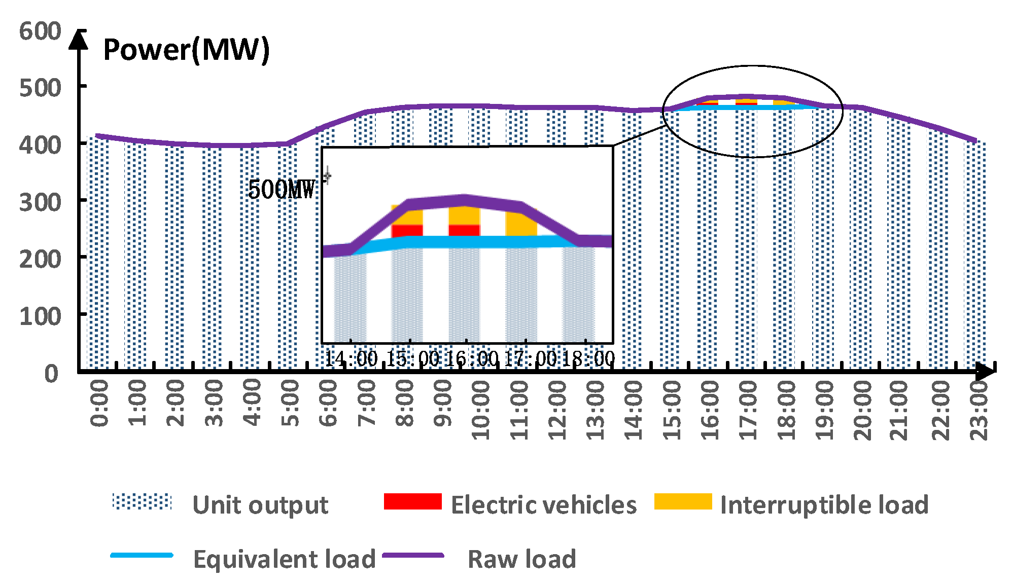
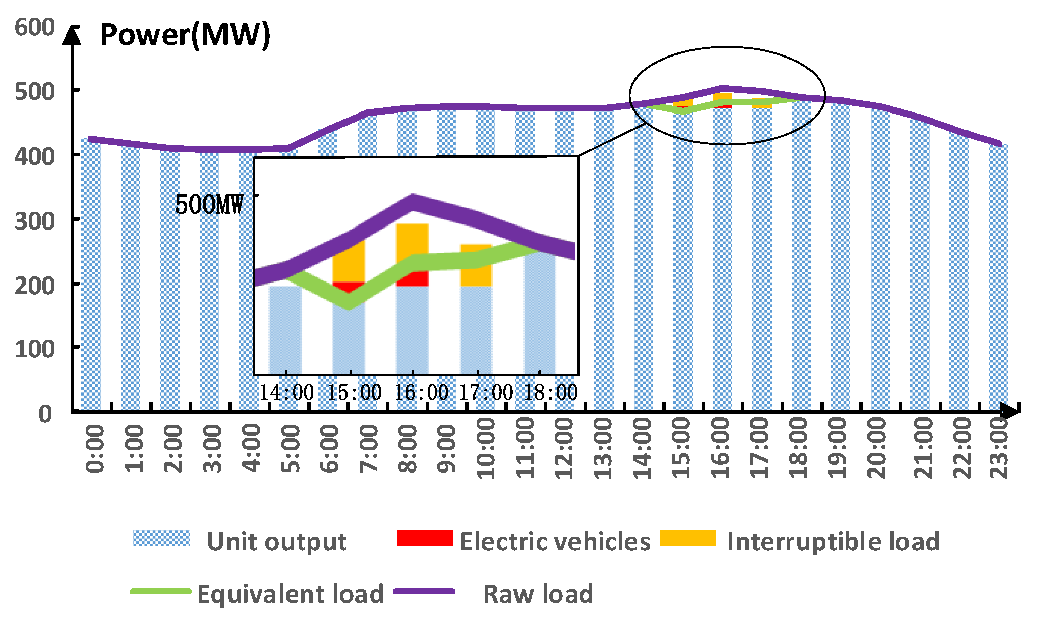
The main objective of demand response resources in peak load reduction is twofold: firstly, to reduce the peak-to-valley difference of grid load so that power generation and consumption tend to balance and avoid power pulling and restriction as far as possible; secondly, to use clean demand-side resources to replace a part of traditional thermal power units to achieve the purpose of energy saving and emission reduction.

(1) When the demand response resource capacity can meet the requirements of power balance during peak load, the system will not experience power shortage, and the response cost is the peak shaving cost, so the lowest demand-side response service cost and the highest carbon emission reduction are taken as the optimization objectives.

Firstly, it is clear that the demand response cost is the change of power revenue before and after load reduction. Before demand response, the revenue of power companies is mainly electricity revenue.

$$I_{n,t}^{before}=r_0{L}_{n,t}^{before}$$

(6)

where $I_{n,t}^{before}$ is the revenue of the electric utility before the demand response resource participates in the peak shaving response; r₀ is the retail electricity price, based on the integrated average electricity price; $L_{n,t}^{before}$ is the load of the nth demand response resource at the moment t before the demand response is implemented.

Demand-side resources participate in peak-shaving response and reduce the utility’s electricity revenue while paying additional demand response costs.

$$\{\begin{array}{l}{I}_{n,t}^{after}=r_0(L_{n,t}^{before}-L_{n,t})-C_{n,t}\\ C_{n,t}=a_n{L}_{n,t}^2+b_n{L}_{n,t}\end{array}$$

(7)

where $I_{n,t}^{after}$ is the revenue of the power company after the demand response resource participates in the peak shaving response; L_n,t is the load reduction of the nth demand response resource at the time; C_n,t is the financial compensation of the power company to the customers participating in the demand response; a_n and b_n are the quadratic and primary coefficients of the compensation amount of the nth demand response resource, respectively.

Therefore, the response cost of demand-side resources during peak load periods is:

$$cos{t}_{n,t}=I_{n,t}^{before}-I_{n,t}^{after}$$

(8)

Bringing Equations (6) and (7) into Equation (8), the relationship between response cost and load reduction is obtained as:

$$cos{t}_{n,t}=a_n{L}_{n,t}^2+(b_n+r_0)L_{n,t}$$

(9)

The cost of peak shaving is:

$$cost={\displaystyle \sum _{n=1}^H{\displaystyle \sum _{t=1}^T[a_n{L}_{n,t}^2+(b_n+r_0)L_{n,t}]}}$$

(10)

where H is the number of demand response resources.

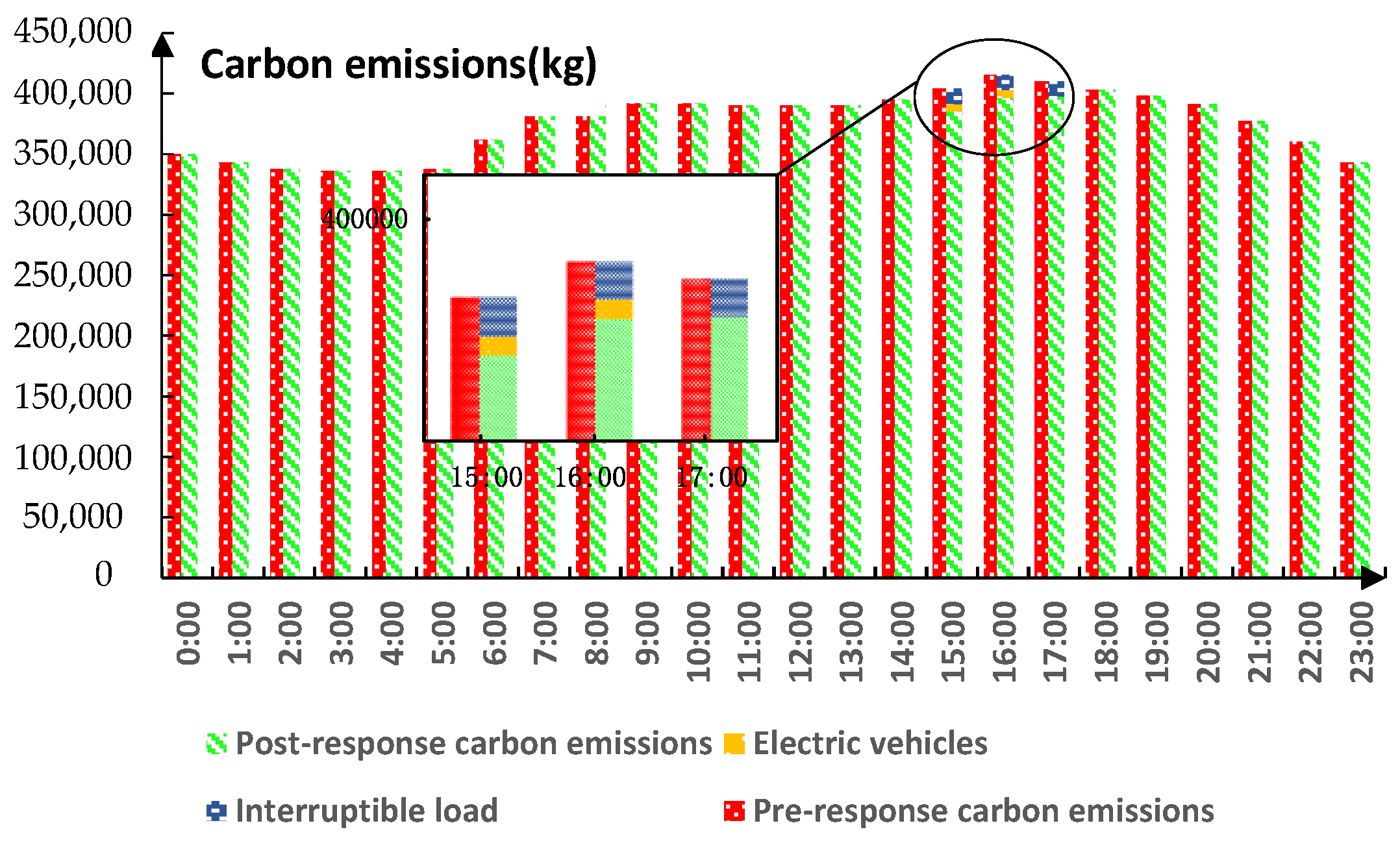
Since there is no direct link between power generation and carbon emissions from coal-fired power plants, it is necessary to first determine the coal consumption of thermal power plants based on the coal consumption coefficients of each unit; then, the carbon content of the coal consumed is determined by selecting the appropriate carbon content coefficient according to the type of coal combusted; and finally, the carbon emissions of thermal power plants are obtained based on the actual carbon generation CO₂ coefficient, i.e., the carbon emission reduction of thermal power plants after the participation of demand response resources in peak shaving is [27]:

$$C={\mu }_1{\mu }_2{\mu }_3{\displaystyle \sum _{n=1}^H{\displaystyle \sum _{t=1}^T{L}_{n,t}}}$$

(11)

where C is the CO₂ emission; μ₁ is the coal consumption factor; μ₂ is the carbon content factor; μ₃ is the carbon generation CO₂ factor.

(2) When the demand response capacity cannot fully meet the requirements of power balance during the peak load period, the minimum peak shaving cost and orderly power consumption management scale, the minimum peak shaving cost and the maximum carbon emission reduction are taken as the optimization objectives. At this time, the peak shaving cost consists of response cost and power shortage cost.

$$\{\begin{array}{l}E={\displaystyle {\displaystyle \sum }_{t=1}^T}{L}_t^{before}-{\displaystyle {\displaystyle \sum }_{n=1}^H}{\displaystyle {\displaystyle \sum }_{t=1}^T}{L}_{n,t}-{\displaystyle {\displaystyle \sum }_{t=1}^T}{P}_t\\ cost={\displaystyle {\displaystyle \sum }_{n=1}^H}{\displaystyle {\displaystyle \sum }_{t=1}^T}[a_n{L}_{n,t}^2+(b_n+r_0)L_{n,t}]+r_{w}E\end{array}$$

(12)

where P_t is the unit output for the time period; E is the amount of power pulling limit; r_w is the unit cost of power shortage.

In the above calculations, it is considered that demand response users can fully respond to the demand side according to the response amount agreed in advance when the load fluctuates violently. However, in practice, there is great uncertainty in the response of each user after the load reduction order is issued. Demand responsive users have three situations: over response, full response, and under response. The first two have little negative impact on the power company. The power company only needs to compensate the responsive users according to Formula (9) according to the agreed load reduction and does not need to pay other fees. When the responding user fails to reduce by a certain amount of load as required, the power company will compensate the user according to the actual load reduction of the user. However, at this time, the power company needs to consider the risk of power shortage caused by demand response and user under response; that is, although the power company reduces the response cost, it needs to bear the risks of re-purchasing high-priced power generation capacity and maintaining network security and stability.

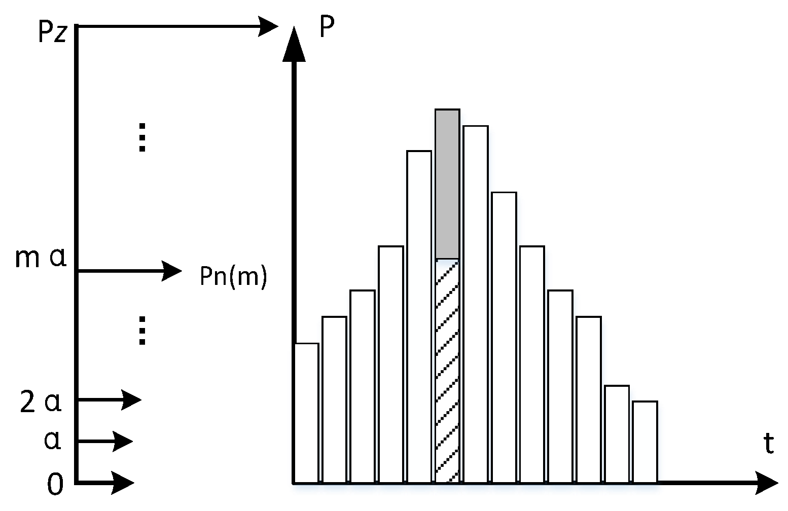
Therefore, when considering the uncertainty of demand response, the actual load reduction is divided into agreed load reduction and random deviation. The peak shaving cost, minimum power limit, and carbon emission reduction are shown in Formulas (13)–(15).

$$cost=\{\begin{array}{l}{\displaystyle {\displaystyle \sum }_{n=1}^H}{\displaystyle {\displaystyle \sum }_{t=1}^T}[a_n{({\stackrel{-}{L}}_{n,t}+{\theta }_{n,t})}^2+(b_n+r_0)·({\stackrel{-}{L}}_{n,t}+{\theta }_{n,t})+r_w{\theta }_{n,t}],{\theta }_{n,t}<0\\ {\displaystyle {\displaystyle \sum }_{n=1}^H}{\displaystyle {\displaystyle \sum }_{t=1}^T}[a_n{\stackrel{-}{L}}_{n,t}^2+(b_n+r_0){\stackrel{-}{L}}_{n,t}],{\theta }_{n,t}\ge 0\end{array}$$

(13)

$$E=\{\begin{array}{l}0,{\theta }_{n,t}\ge 0\\ {\displaystyle {\displaystyle \sum }_{t=1}^T}{L}_t^{before}-{\displaystyle {\displaystyle \sum }_{n=1}^H}{\displaystyle {\displaystyle \sum }_{t=1}^T}({\stackrel{-}{L}}_{n,t}+{\theta }_{n,t})-{\displaystyle {\displaystyle \sum }_{t=1}^T}{P}_t,{\theta }_{n,t}<0\end{array}$$

(14)

$$C={\mu }_1{\mu }_2{\mu }_3{\displaystyle \sum }_{n=1}^H{\displaystyle \sum }_{t=1}^T({\stackrel{-}{L}}_{n,t}+{\theta }_{n,t})$$

(15)

where ${\stackrel{-}{L}}_{n,t}$ is the agreed load reduction of demand response resources; ${\theta }_{n,t}$ is the stochastic deviation amount.

2.2.2. Constraints

Electricity users participate in response during the peak load period to obtain economic benefits while reducing the sense of electricity experience to a certain extent, so the response satisfaction of users participating in demand response must be considered in the demand response model, so the energy response constraint and time response constraint are added to the model, and the specific constraints are as follows.

(1) Load reduction constraint. The load shedding energy of a demand response resource should be less than the maximum capacity it can provide and should also be greater than 0 (in a responsive state).

$$0\le L_{n,t}\le {\mu }_{n,t}{D}_{n,t}^{max}$$

(16)

where $D_{n,t}^{max}$ represents the maximum load reduction of the n_st demand response resource in the time period; μ_n,t is energy invocation status in the time period, 1 means invoked, 0 means not invoked.

(2) Response duration constraint. When receiving dispatching instructions from the trading center, the demand response resources in the operation area need to be dispatched. If the time response characteristics are not controlled, it will bring greater pressure to the actual operation of suppliers and also affect the basic electricity demand of customers. In order to facilitate customers to adjust their production and living electricity plans as well as to take into account the technical characteristics of each demand response resource, the response time should be limited to a certain range.

$$T_n^{min}\le T_n^{on}\le T_n^{max}$$

(17)

where T_n represents the response time of the nth demand response resource in the scheduling cycle; $T_n^{min}$ and $T_n^{\max }$ represent its minimum and maximum response times in the scheduling cycle.

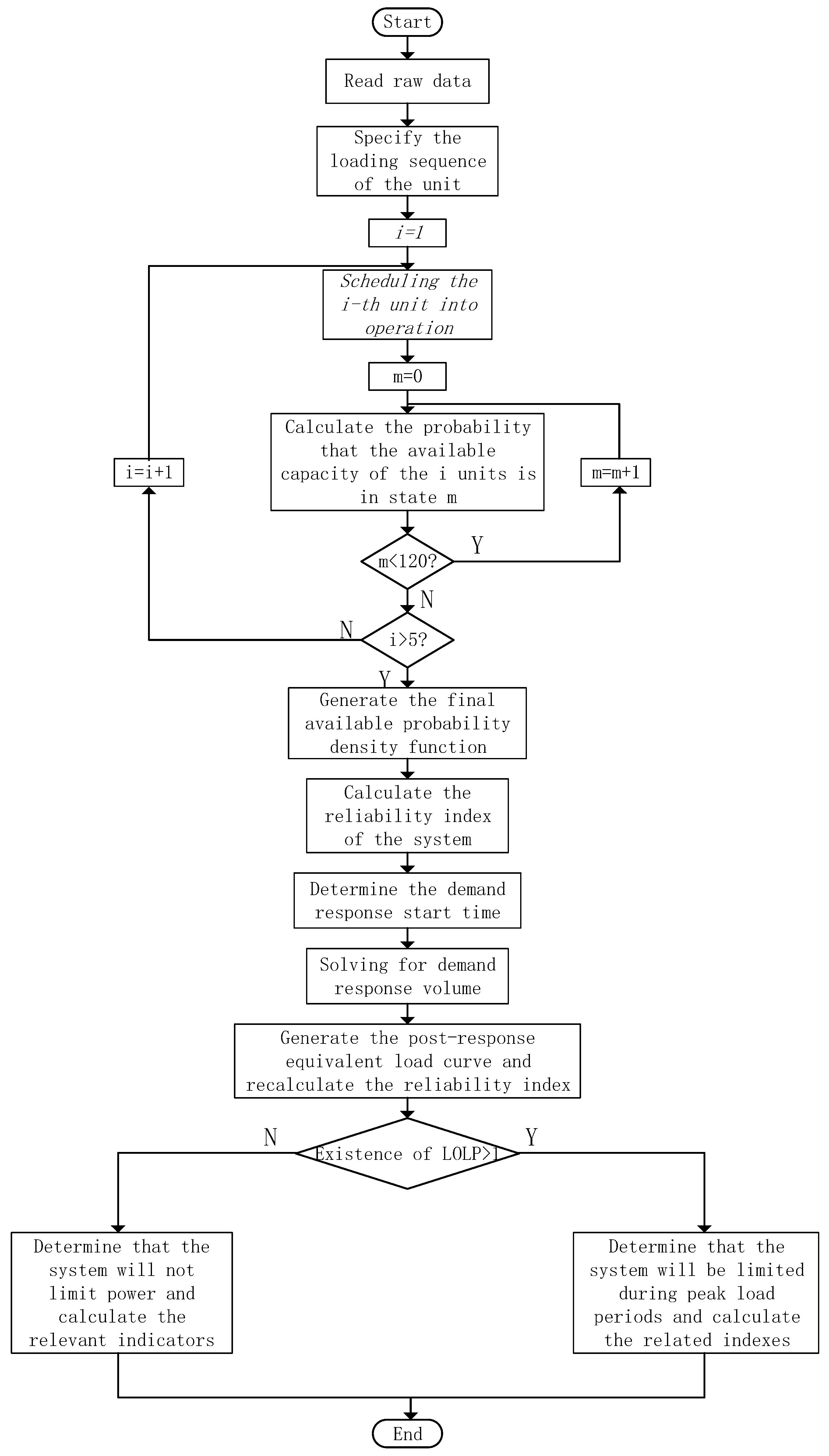
In summary, the flow of demand response analysis taking into account unit uncertainty is shown in Figure 3.

3. Results and Discussion

In this paper, the complex objective function and constraints in the power system dispatch model are transformed into a linear programming problem and solved using a Cplex solver in the solution process, which reduces the difficulty of solving the dual uncertainty dispatch model. Two typical peak shaving scenarios of the IEEE30 node system are selected for demand response analysis. The total installed capacity of the system is 480 MW, and the detailed parameters of the generating units are shown in

Table 1. Generator set parameters.

Unit Number	Capacity(MW)	Forced Outage Rate	Forced Derate Rate
1	160	0.04	0.025
2	100	0.026	0.02
3	60	0.017	0.01
4	80	0.02	0.013
5	40	0.01	0.005
6	40	0.01	0.005

[28,29].

The unit commissioning sequence is determined according to the fuel cost, and the available capacity probability density function of the system is generated based on the forced outage rate of each unit, and the probability of this system operating at each available capacity state is shown in

Table 2. The probability density of available capacity.

Available Capacity (MW)	Probability	Available Capacity (MW)	Probability
0~216	0.0001	416	0.0222
220~276	0.0025	420	0.0168
280~316	0.0037	424~436	0.0005
320~372	0.0383	440~444	0.0337
376	0.0011	448~452	0.0084
380	0.0229	456~460	0.0109
384~396	0.0008	464~476	0.0083
400	0.0149	480	0.8143
404~412	0.0005

.

Assuming that the demand response resources available for peak shaving in this system are both electric vehicles and interruptible loads, it can be approximated that the deviations of both load reductions obey a normal distribution with a mean of zero, and their standard deviations are shown in

Table 3. Demand response resource parameters.

Demand Response Resources	Electric Vehicles	Interruptible Load
a ($/MW·h)	0.9	0.95
b ($/MW·h)	80	85
Duration	2	3
Response capacity/MW	7.5	15
Standard deviation	0.63	0.1

.

The compensation coefficient of electric vehicles is large; that is, when the uncertainty of demand response is not considered, the response cost of electric vehicles is higher. The standard deviation of the interruptible load is small; that is, considering the uncertainty of demand response, the response reliability of interruptible load is higher, and the estimated power shortage cost is lower [30].

3.1. Peak Shaving Scenario 1

The reliability index of scenario 1 is solved according to Equations (2)–(4), where the expected value of time-sharing power shortage is shown in

Table 4. Expected loss of energy.

Time	EENS (MW)	Time	EENS (MW)	Time	EENS (MW)
0:00	5.50	8:00	12.39	16:00	16.51
1:00	4.79	9:00	12.78	17:00	18.95
2:00	4.27	10:00	12.78	18:00	15.65
3:00	4.12	11:00	12.39	19:00	12.78
4:00	4.12	12:00	12.39	20:00	12.67
5:00	4.27	13:00	12.39	21:00	9.79
6:00	7.19	14:00	11.65	22:00	6.93
7:00	10.84	15:00	12.02	23:00	4.79

.

From Table 4, it can be seen that the load from 16:00 to 18:00 is greater than the maximum value of unit output, so there must be a loss of load in this period, i.e., the probability of power shortage is 1. The load in the rest of the period is smaller, and the probability of power shortage is very small after considering the uncertainty of unit output, so it can be considered that the load and unit output in these periods can be balanced. The demand response resources start to respond at 16:00, and the response results are shown in Figure 4 and

Table 5. Loss of energy probability.

Time	LOLP before Demand Response	LOLP after Demand Response	Service Fees ($)	Carbon Emission Reduction (kg)
16:00	1	0.1775	1493.596	13,620.75
17:00	1	0.1857	1748.422	15,633.75
18:00	1	0.1647	1488.75	12,375

.

The difference between the original load curve and the post-response equivalent load curve in the interval from 16:00 to 18:00 in Figure 4 is the load reduction of the system after the operation of demand response resources.

As can be seen from Figure 4 and Table 5, after the implementation of the demand response in Scenario 1, the active output of the generating units can basically meet the load demand, and the probability of power shortage during peak hours also decreases from 1 to within 0.2, i.e., it can be approximated that demand response makes Scenario 1 achieve supply–demand balance even during peak load periods without the need to implement power pulling and restriction measures. The cost of the peak-shaving demand response side service is $4730.77, and the carbon emission reduction is 42,169.05 kg.

In order to compare the effect of demand response uncertainty on the effect of peak shaving, a new optimization scenario is set up, in which the cost of peak shaving is considered with demand response uncertainty. Then, the range of two demand response resources output is obtained by changing the reliability index of demand response resources, as shown in Figure 5.

In Figure 5, the upper cluster of curves shows the fluctuation range of interruptible load output, and the lower cluster of curves shows the fluctuation range of electric vehicle output. It can be seen that after considering the demand response resource response uncertainty, the response of interruptible load with higher reliability increases within its regulation range (curve cluster changes upward), and the response of electric vehicle with lower reliability decreases (curve cluster changes downward), and its response fluctuates within a certain range.

3.2. Peak Shaving Scenario 2

The time-sharing power shortage expectations for Scenario 2 are shown in

Table 6. Expected loss of energy.

Time	EENS (MW)	Time	EENS (MW)	Time	EENS (MW)
0:00	6.61	8:00	14.23	16:00	39.31
1:00	5.64	9:00	14.63	17:00	32.68
2:00	5.10	10:00	14.63	18:00	24.29
3:00	4.93	11:00	14.23	19:00	18.38
4:00	4.93	12:00	14.23	20:00	14.53
5:00	5.10	13:00	14.23	21:00	11.47
6:00	8.43	14:00	15.32	22:00	8.17
7:00	12.59	15:00	25.20	23:00	5.64

.

From Table 6, we can see that the load from 15:00 to 19:00 is greater than the maximum value of unit output, so the load loss state must occur in this period, i.e., the probability of power shortage is 1. The load in the rest of the period is smaller, and the probability of power shortage is very small after considering the uncertainty of unit output, so we can assume that the load and unit output in these periods can be balanced. The demand response resource starts to respond at 15:00, and the response results are shown in Figure 6 and

Table 7. Loss of energy probability.

Time	LOLP before Demand Response	LOLP after Demand Response	Service Fees ($)	Carbon Emission Reduction (kg)
15:00	1	0.1857	2139.375	18,562.5
16:00	1	1	2139.375	18,562.5
17:00	1	1	1488.75	12,375

.

The difference between the original load curve and the equivalent load curve after response in the interval from 15:00 to 17:00 in Figure 6 is the load reduction of the system after the operation of demand response resources.

As can be seen from Figure 6 and Table 7, after the implementation of the demand response in Scenario 2, the generating units still cannot meet the demand of the load at all times, except at 15:00, when the probability of power shortage decreases to 0.1857, but the probability of power shortage in the rest of the time is not significantly reduced, i.e., it is still necessary to adopt the method of power pulling and restriction to make the system supply and demand balance during the peak hours. The response cost is $5767.5, the shortage cost is $79,860, and the carbon emission reduction is 49,500 kg. The amount of power pulled and restricted before and after the demand response and the carbon emission of thermal power plants are shown in Figure 7 and Figure 8.

According to the comparison of the system pulling power limit before and after demand response, it can be seen that because the demand response resources are in the response state from 15:00 to 17:00, the power limit after the response in Figure 7 is significantly reduced compared with that before the response, of which 15:00 can be basically considered as a complete response; there is no demand response measure in the period from 18:00 to 19:00, so the power limit is not reduced. Therefore, demand response can effectively reduce the outage range of the system. Figure 8 shows that the carbon emissions of thermal power plants in this power system are reduced after the demand response resources are involved in peak shaving optimal dispatch.

Setting up a new optimization scenario that considers demand response uncertainty, a comparison of the response resource output is shown in

Table 8. Deterministic demand response volume.

Time	Response Volume (MW)
	Electric Vehicles	Interruptible Load
15:00	7.5	15
16:00	7.5	15
17:00	0	15

and

Table 9. Uncertain demand response volume.

Time	Response Volume (MW)
	Electric Vehicles	Interruptible Load
15:00	7.38	14.79
16:00	7.29	15
17:00	0	15

.

As can be seen from Table 8 and Table 9, when all the demand response resources in the scenario with a heavy peak-shaving task need to be put into operation, the response volume is only equal to or less than the response resource capacity in two cases after considering the demand response uncertainty, and when the response volume is less than the response resource capacity, it will affect the peak-shaving effect of the demand response resources.

4. Conclusions

This paper investigates the impact of uncertain thermal units and demand response resources on power system dispatch and emission reduction problems, and the following conclusions are obtained.

• Considering the impact of power supply uncertainty on unit output, a probabilistic model is established for thermal power units by using a time-series stochastic production simulation algorithm, a probabilistic active output curve is re-established, a unit day-ahead output model is constructed, uncertain demand response resources are involved in power system dispatch as a virtual power supply, and a power demand response dispatch model accounting for double uncertainty is proposed.
• The uncertainty of thermal power unit output leads to the increase in peak valley difference of the system. In this example, the probability of system power shortage is set to be less than 0.2 as the supply–demand balance. The peak valley dispatching period is 3–4 h, which is close to the maximum duration of demand response resources. There are two situations when demand response resources participate in power system dispatching as a virtual power source: The demand response capacity is fully responsive when it meets the maximum power difference during the peak load period, and the response cost is proportional to the load reduction. When the demand response capacity cannot meet the peak shaving demand, the system still needs to limit power in some areas after the response, but the orderly power consumption scale is reduced. The dispatching model in this paper calculates the response volume, service cost, and carbon emission of each period of the system and provides decision-making opinions for the power dispatching department.
• In this example, the response power range of electric vehicles is 6.82–7.5 MW; The power range of interruptible load response is 9.01–14 MW. Through the analysis of demand response uncertainty, it is found that when the peak shaving task is light and the demand response resources do not need to be put into operation, the response uncertainty will lead to an increase in the response volume of resources with high reliability, resulting in an increase in the response cost. When the peak shaving task is heavy and all demand response resources need to be put into operation, the under-response caused by response uncertainty will affect the peak shaving effect. Therefore, when allocating demand response resources for the system, it is necessary to fully consider the reliability index of demand response resources.

References

1. Zheng, J.; Hu, M.; Hu, Z.; Hu, M. A Distribution Network Planning Model Considering Reliability and Demand Response. J. Electr. Power Sci. Technol. 2019, 34, 173–182. [Google Scholar]
2. Tan, Z. Real-Time Demand Response for Electricity; China Electric Power Press: Beijing, China, 2021; p. 25. [Google Scholar]
3. He, S.; Xu, Y.; Chen, S.; Yuan, J.; Gong, F. The Development Effectiveness of China’s Power Demand Response and the Outlook of the 14th Five-Year Plan. Electr. Demand-Side Manag. 2021, 23, 1–6. [Google Scholar]
4. Li, J.; Chen, X. An Analysis of Demand-side Response Technologies. China Foreign Energy 2021, 26, 16–22. [Google Scholar]
5. Li, Z.; Han, A.; Zhou, S.; Chen, Z.; Zhang, Z. Optimal Scheduling of Integrated Energy Systems with Calculation and Integrated Demand Response. Power Syst. Prot. Control 2021, 49, 36–42. [Google Scholar]
6. Wang, B.; Ye, B.; Zhu, L.; Han, J.; Ye, B.; Cheng, Q.; Gao, C. Practice and Exploration of Electricity Demand Response in China under Market Environment. Power Demand Side Manag. 2021, 23, 91–95. [Google Scholar]
7. Liu, C.; Qu, J.; Shi, W. A New Energy Consumption Capacity Assessment Method Based on Stochastic Production Simulation. Chin. J. Electr. Eng. 2020, 40, 3134–3144. [Google Scholar]
8. An, M.; Zhang, Z.; Chen, Z.; Huang, R.; Ding, K.; Dong, H. Stochastic Production Simulation Study of Power Systems Containing Photovoltaic-photovoltaic Co-generation. Renew. Energy 2019, 37, 1603–1610. [Google Scholar]
9. Cao, B.; Lv, G.; Wang, N.; Jia, D. Research and Application of Demand Response under Optimal Scheduling of Integrated Energy Systems. Electr. Demand Side Manag. 2021, 23, 45–50. [Google Scholar]
10. Cui, Y.; Xiu, Z.; Liu, C.; Zhao, Y.; Tang, Y.; Chai, X. Two-layer Optimal Dispatch of Power System with Demand Response and Fire-storage Deep Peaking Pricing Strategy. Chin. J. Electr. Eng. 2021, 41, 4403–4415. [Google Scholar]
11. Talebi, M.; Hatami, A. Optimal Scheduling of Generation and Demand Response Resources with Considering Load Uncertainty. In Proceedings of the Iranian Conference on Electrical Engineering, Mashhad, Iran, 8–10 May 2018. [Google Scholar]
12. Wynn, S.L.L.; Boonraksa, T.; Boonraksa, P.; Marungsri, B. Optimal Distribution Level of Energy Management Considering Generation Uncertainties and Demand Response. In Proceedings of the 2021 International Conference on Power, Energy and Innovations, Nakhon Ratchasima, Thailand, 20–22 October 2021; pp. 29–32. [Google Scholar] [CrossRef]
13. Wang, L.; Hou, C.; Ye, B.; Wang, X.; Yin, C.; Cong, H. Optimal Operation Analysis of Integrated Community Energy System Considering the Uncertainty of Demand Response. Trans. Power Syst. 2021, 36, 3681–3691. [Google Scholar] [CrossRef]
14. Li, Y.; Han, M.; Yang, Z.; Li, G. Coordinating Flexible Demand Response and Renewable Uncertainties for Scheduling of Community Integrated Energy Systems with an Electric Vehicle Charging Station: A Bi-Level Approach. Trans. Sustain. Energy 2021, 12, 2321–2331. [Google Scholar] [CrossRef]
15. Wu, S.; Feng, Y.; Wu, K.; Lu, W.; Zhao, C.; Luo, C. An Operational Evaluation Method for Power Systems Containing High Proportion of New Energy Based on Exchange Convolution. China Electr. Power 2019, 52, 25–31. [Google Scholar]
16. Zhu, R.; Hu, B.; Xie, K.; Zhu, Q.; Zhao, D.; Niu, T.; Li, C.; Sun, Y. Time-series Stochastic Production Simulation of a Multi-energy Power System Containing Wind-photovoltaic-photothermal-hydro-fired-energy Storage. Power Grid Technol. 2020, 44, 3246–3253. [Google Scholar]
17. Zhou, M.; Li, Y.; Li, G. A Two-tier Decision Model for Day-ahead Generation-standby Based on Stochastic Production Simulation. Power Grid Technol. 2019, 43, 1606–1613. [Google Scholar]
18. Luo, D.; Liu, Y. Assessment of Photovoltaic Consumption Capacity Based on Stochastic Production Simulation. Distrib. Energy 2018, 3, 9–15. [Google Scholar] [CrossRef]
19. Liao, Q.; Xie, K.; Hu, B. Time-series Stochastic Production Simulation of Power Systems Containing Wind Power and Energy Storage. Power Grid Technol. 2017, 41, 2769–2776. [Google Scholar]
20. Wang, L.; Zhu, Y.; Wu, X.; Yan, L.; Li, Y. Confidence Capacity Assessment of Wind Power Based on Time-series Stochastic Production Simulation. J. Power Syst. Autom. 2018, 30, 114–119. [Google Scholar]
21. Li, L.; Yan, Y.; Luo, Y.; Zhang, T.; Zhang, Z.; Lv, T.; Lin, Z. Invitational Demand Response Mechanism Based on Smart Contract. Zhejiang Electr. Power 2022, 41, 20–29. [Google Scholar]
22. Zhang, G.; Xue, S.; Fan, M.; Zhang, H. The Design of Demand Response Market-based Trading Mechanism for China’s Electricity Market. Power Constr. 2021, 42, 132–140. [Google Scholar]
23. Zhang, Y. Day-ahead Economic Dispatch of An Integrated Energy System with Calculation and Price-based Demand Response. Jilin Power 2020, 48, 20–23. [Google Scholar]
24. Guo, M.; Lv, R.; Fei, F.; Chen, T. Economic Dispatch of Coupled Electric-thermal-water Multi-energy System Considering Electric Vehicles and Demand Response. China Power 2022, 4, 1–10. Available online: http://kns.cnki.net/kcms/detail/11.3265.tm.20211210.1934.008.html (accessed on 25 May 2022).
25. Yan, Q.; Li, Y.; Liu, X. Simulation of Resident Demand Response Considering User Response Uncertainty. In Proceedings of the China International Conference on Electricity Distribution, Shanghai, China, 7–9 April 2021; pp. 1010–1014. [Google Scholar] [CrossRef]
26. Majidi, M.; Zare, K. Integration of Smart Energy Hubs in Distribution Networks Under Uncertainties and Demand Response Concept. Trans. Power Syst. 2019, 34, 566–574. [Google Scholar] [CrossRef]
27. Bai, J.; Li, F. Study on Carbon Emission Modeling of Thermal Power Plants in the Beijing-Tianjin-Tanggu Region. Energy Environ. Prot. 2013, 27, 15–19. [Google Scholar]
28. Zou, B.; Li, D. Stochastic production simulation of power system with wind farms based on effective capacity distribution. Proc. CSEE 2012, 32, 23–31187. [Google Scholar]
29. Luo, D. Stochastic production simulation under the background of coordinated operation of high proportion renewable energy and energy storage. North China Electr. Power Univ. 2019, 12, 14–16. [Google Scholar]
30. Niu, W.; Li, Y.; Wang, B. Demand Response Virtual Power Plant Modeling Considering Uncertainty. Chin. J. Electr. Eng. 2014, 34, 3630–3637. [Google Scholar] [CrossRef]
Figure 1. Three-state unfolding type formulation of unit loading.
Energies 15 04588 g001
Figure 2. Schematic diagram of sequential stochastic production simulation.
Energies 15 04588 g002
Figure 3. Demand response optimization peak shaving algorithm flowchart.
Energies 15 04588 g003
Figure 4. System operation status before and after demand response.
Energies 15 04588 g004
Figure 5. Fluctuating range of demand response resources.
Energies 15 04588 g005
Figure 6. System operation status before and after demand response.
Energies 15 04588 g006
Figure 7. Under-response power limit.
Energies 15 04588 g007
Figure 8. Carbon emissions before and after response.
Energies 15 04588 g008