Numerical Study on Aerodynamic Characteristics of Heavy-Duty Vehicles Platooning for Energy Savings and CO₂ Reduction

Abstract

This study aims to analyze the aerodynamic interaction between moving vehicles platooning with the change in the platooning conditions on a freeway. The effect of the vortex generated by the forward vehicle reduces the value of the stagnation pressure generated at the front of the rear vehicle, which effectively reduces drag on the driving vehicle. To elucidate this, a total of four vehicles were applied to platooning at a speed of 100 km/h by altering the gap distance of heavy-duty vehicles (HDVs) such as 0.5 Length (L), 1 L, 1.5 L, 2.0 L, and 2.5 L under the conditions of 1 L equal to 13.16 m. The stagnation pressure at the front of the following vehicle (FV) was reduced, and quantitative analysis of drag force generated at each leading vehicle (LV) and following vehicle that is platooning exhibited a reduction of about 51%, 56%, and 52%, respectively, when compared to the single moving HDV. This is considered as a reduction in engine power for the driving vehicle. Taken together, these results are effective in improving fuel efficiency and reducing CO₂, a representative greenhouse gas, and predicting fuel and CO₂ reduction based on HDV annual mileage according to the highway conditions and logistics.

1. Introduction

Greenhouse gas reduction has emerged as one of the biggest global problems. The six primary greenhouse gases are CO₂, CH₄, N₂O, HFCs, PFCs, and SF₆, which cause the greenhouse effect. Among them, CO₂ was increased by 80% in annual emissions from 1970 to 2004. To reduce greenhouse gas (GHG) emissions, the world government has established decarbonization policies, and automobiles are moving away from internal combustion engines in line with policies. However, due to logistics on the road it would take a long time to change internal combustion engine vehicles to eco-friendly vehicles. Previous studies have examined actively utilizing aerodynamic characteristics to improve the fuel efficiency of internal combustion engines. Representatively, recent studies were performed on mounting an airfoil-shaped spoiler at the tail end of a vehicle [1], mounting a vortex generator [2], attempting to change the rear design of the vehicle [3], mounting an air duct [4], and securing the seal of the side window of the vehicle [5]. In particular, research and development applying aerodynamic characteristics such as a roof fairing system is representative [6]. Recently, as autonomous driving such as V2X (Vehicle-to-Everything) became an issue, European countries tried to solve the problem of air resistance that occurs during driving rather than reducing air resistance by changing the vehicle’s exterior. For example, in 2011, the SARTRE project [7], an empirical study conducted for GHG reduction using the aerodynamic characteristics, occurred during platooning of the freight vehicles. However, the technology for controlling the distance between vehicles was not developed at that time, so the project could only confirm the possibility of GHG reduction through platooning. Therefore, the SARTRE project, an empirical study, researched controlling the distance between vehicles by lowering the freight vehicle to 6 m, thereby confirming the possibility of improving fuel economy and reducing GHG. Those effects lead to the reduction in logistics costs [8]. In addition, the Korean government leads the Truck Platooning Project of Korea (TROOP) [9], an empirical study for platooning large freight vehicles. This project has been conducted to control the distance between vehicles at about 15 m. Based on V2X for the safety of autonomous vehicles, diversified platooning safety research is underway, such as distance control of ACC (Adaptive Cruise Control) [10], platooning for CACC (Cooperative Adaptive Cruise Control) [11,12], analysis of acceleration driving of lead vehicles during platooning [13], and emergency braking control [14]. Previous studies demonstrated that platooning driving might contribute to an eco-friendly road environment by reducing air resistance. Therefore, the objective of this study is to understand the variation in aerodynamic characteristics of each model vehicle in platooning by analyzing the change in pressure and drag force of each vehicle in platooning.

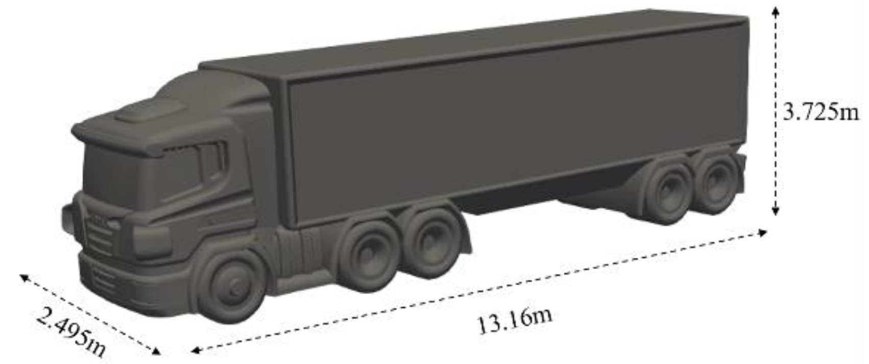
2. Description of the Model Vehicle with Its Numerical Grid

In this study, we chose the SCANIA R-series heavy-duty vehicle with a 13.0 liter diesel engine with its maximum brake power, 500 hp. This model vehicle has been used for on-road tests for aerodynamic performance analysis of vehicle platooning in previous empirical studies, due to occupying a large position in the transportation and logistics market worldwide [15,16]. The simplified model vehicle was used for this numerical study, and the solid model with the geometric dimensions 13.16 m × 2.495 m × 3.725 m (Length × Width × Heigth) is given in Figure 1.

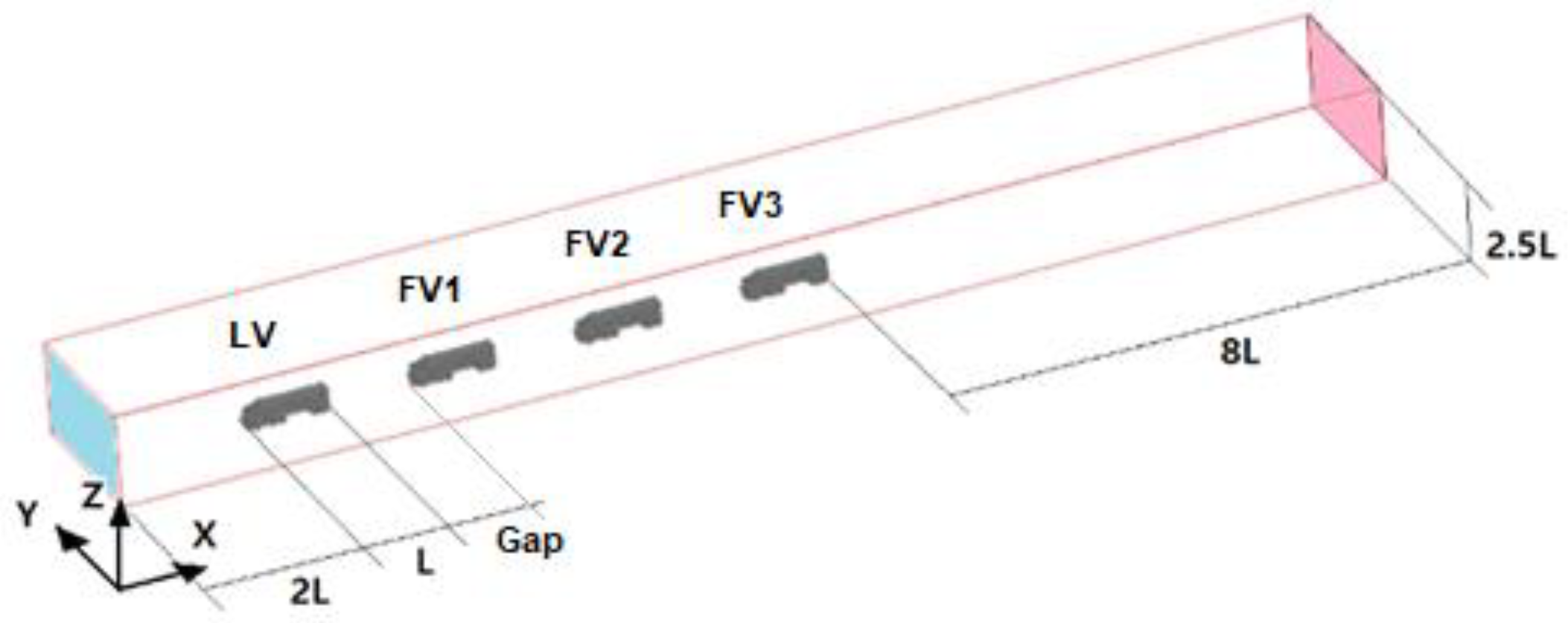
2.1. Numerical Domain and Its Conditions

The numerical domain size was defined as shown in Figure 2. Especially, 8 L was given at the rear side of the last model vehicle for stable convergence on the simulation result.

The airflow field was assumed as a 3-dimensional steady incompressible and turbulent flow field for the numerical calculation. The details of the initial and boundary conditions are given in

Table 1. Boundary and initial conditions on the control volume.

Boundary Surface	Boundary and Initial Conditions
Inlet	Velocity boundary: 100 km/h
Outlet	Pressure boundary: ambient pressure, 1 atm
Sides and top	Open boundary: symmetric conditions
Ground	Moving boundary condition: 100 km/h
Model surface	No-slip wall

. The inlet was defined as the velocity boundary with the plugged flow condition, and the outlet was assumed as fully developed and defined as the pressure boundary with the ambient condition. The moving boundary was set to the ground with the same speed as the inlets.

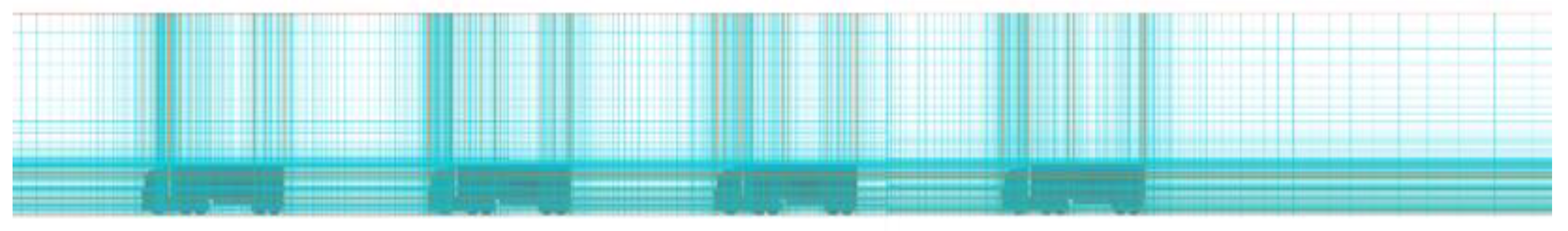
2.2. Numerical Grid of the Physical Model

The CAD-to-CFD method [17] in conjunction with the orthogonal grid was used for the discretization of the physical domain in this study. First, the 3D CAD program, Pro-Engineers, was used as solid model of the vehicle and it was transferred into the numerical domain to generate the hexagonal meshes in the Cartesian coordinate system.

Figure 3 shows a typical grid in the numerical domain with four model vehicles keeping their distance (1 L) in between. For the optimum grid in the domain, the grid convergence test was conducted by thorough grid dependence evaluation with different iterations and very nicely converged with the cut-off error of the residual fraction of the main properties less than 0.01%. The optimum grid size was decided to be (658 × 99 × 87), and the total number of the grid was 5,667,354.

3. Numerical Scheme and Its Condition

The general-purpose FVM (finite volume method) CFD code, PHOENICS (ver.2020), was used for a numerical calculation of the turbulent incompressible flow field. The 3-dimensional Naiver–Stokes equations were solved with the KECHEN turbulent model (Chen–Kim κ-ε model), a modified standard κ-ε turbulent model that had good agreement with experimental data [18]. The turbulent no-slip condition near the solid boundary was modeled by logarithmic law.

The airflow field for the analysis was defined as follows:

• Quasi-3D flow.
• Turbulent flow.
• Incompressible flow.
• Steady flow.

3.1. Governing Equations

The governing equation for the steady, incompressible, and turbulent flow fields is given below:

(1)

Continuity equation:

$$\frac{\partial {\mathrm{U}}_{\mathrm{i}}}{\partial {\mathrm{x}}_{\mathrm{i}}}+\frac{\partial {\mathrm{U}}_{\mathrm{j}}}{\partial {\mathrm{y}}_{\mathrm{i}}}+\frac{\partial {\mathrm{U}}_{\mathrm{k}}}{\partial {\mathrm{z}}_{\mathrm{i}}}=0$$

(1)

(2)

Momentum equation:

$$\frac{\partial {\mathrm{U}}_{\mathrm{i}}}{\partial \mathrm{t}}+\frac{\partial }{\partial {\mathrm{x}}_{\mathrm{j}}}\left({\mathrm{U}}_{\mathrm{i}}{\mathrm{U}}_{\mathrm{i}}\right)=-\frac{1}{\mathsf{\rho }}\frac{\partial \mathrm{P}}{\partial {\mathrm{x}}_{\mathrm{i}}}+\frac{\partial \mathrm{U}}{\partial {\mathrm{x}}_{\mathrm{j}}}\left[\mathrm{v}\left(\frac{\partial {\mathrm{U}}_{\mathrm{i}}}{\partial {\mathrm{x}}_{\mathrm{j}}}+\frac{\partial {\mathrm{U}}_{\mathrm{j}}}{\partial {\mathrm{x}}_{\mathrm{i}}}\right)-\overline{{\mathrm{u}}_{\mathrm{i}}{\mathrm{u}}_{\mathrm{j}}}\right]-{\mathrm{g}}_{\mathrm{i}}$$

(2)

where $-\overline{{\mathrm{u}}_{\mathrm{i}}{\mathrm{u}}_{\mathrm{j}}}={\mathrm{v}}_{\mathrm{t}}\left(\frac{\partial {\mathrm{U}}_{\mathrm{i}}}{\partial {\mathrm{x}}_{\mathrm{j}}}+\frac{\partial {\mathrm{U}}_{\mathrm{j}}}{\partial {\mathrm{x}}_{\mathrm{i}}}\right)-\frac{2}{3}{\mathrm{k}\mathsf{\delta }}_{\mathrm{ij}}$.

(3)

κ-ε turbulent energy model (KECHEN);

-

Turbulent kinetic energy equation:

$$\frac{\partial }{\partial {\mathrm{x}}_{\mathrm{i}}}\left({\mathrm{U}}_{\mathrm{j}}\mathrm{k}\right)=\frac{\partial }{\partial {\mathrm{x}}_{\mathrm{i}}}\left[\left(\mathrm{v}+\frac{{\mathrm{v}}_{\mathrm{t}}}{{\mathsf{\sigma }}_{\mathrm{k}}}\right)\frac{\partial \mathsf{\epsilon }}{\partial {\mathrm{x}}_{\mathrm{j}}}\right]+\mathrm{G}-\mathsf{\epsilon }$$

(3)

where $\mathrm{G}=-\overline{{\mathrm{u}}_{\mathrm{i}}{\mathrm{u}}_{\mathrm{j}}}\frac{\partial {\mathrm{U}}_{\mathrm{i}}}{\partial {\mathrm{x}}_{\mathrm{j}}},{ \mathrm{v}}_{\mathrm{t}}={\mathrm{C}}_{\mathsf{\mu }}\frac{{\mathrm{k}}^2}{\mathsf{\epsilon }}$.

-

Energy dissipation equation:

$$\frac{\partial }{\partial {\mathrm{x}}_{\mathrm{i}}}\left({\mathrm{U}}_{\mathrm{j}}\mathsf{\epsilon }\right)=\frac{\partial }{\partial {\mathrm{x}}_{\mathrm{i}}}\left[\left(\mathrm{v}+\frac{{\mathrm{v}}_{\mathrm{t}}}{{\mathsf{\sigma }}_{\mathsf{\epsilon }}}\right)\frac{\partial \mathsf{\epsilon }}{\partial {\mathrm{x}}_{\mathrm{j}}}\right]+\frac{\mathsf{\epsilon }}{\mathrm{k}}\left({\mathrm{C}}_{\mathsf{\epsilon }1}\mathrm{G}-{\mathrm{C}}_{\mathsf{\epsilon }2}\mathsf{\epsilon }\right)$$

(4)

where $\left({\mathrm{C}}_{\mathsf{\mu }}=0.09,{ \mathrm{C}}_{\mathsf{\epsilon }1}=1.15,{ \mathrm{C}}_{\mathsf{\epsilon }2}=1.92,{ \mathsf{\sigma }}_{\mathrm{k}}=1.0,{ \mathsf{\sigma }}_{\mathsf{\epsilon }}=1.0\right)$.

${\mathrm{v}}_{\mathrm{t}}$ is turbulent kinematic viscosities, ${\mathsf{\sigma }}_{\mathrm{k}},{ \mathsf{\sigma }}_{ϵ}$ Prandtl number connected to the diffusivity of K and ε to eddy viscosity [18].

3.2. Aerodynamic Pressure Drag

The drag force (F_D) and drag coefficient (C_D) of the model vehicle are calculated using the following equations.

-

Drag force (F_D)

$${\mathrm{F}}_{\mathrm{D}}={\mathrm{C}}_{\mathrm{D}}·\frac{1}{2}·{\mathsf{\rho }}_{\mathrm{air}}·{\mathrm{A}}_{\mathrm{y}}·{\mathrm{V}}_{\mathrm{HDV}}^2$$

(5)

where A_y is the projected area of the model vehicle in the longitudinal direction.

-

Drag coefficient (C_D)

$${\mathrm{C}}_{\mathrm{D}}=\frac{2{\mathrm{F}}_{\mathrm{D}}}{{\mathsf{\rho }}_{\mathrm{air}}·{\mathrm{A}}_{\mathrm{y}}·{\mathrm{V}}_{\mathrm{HDV}}^2}$$

(6)

3.3. Fuel Savings and CO₂ Reduction

3.3.1. Traction Power Saved on Each Model Vehicle Platooning

The reduction in the tractive power of each model vehicle platooning compared to the single moving vehicle (SV) can be calculated by Equation (7) [19].

-

Tractive power saved,

$${\mathrm{PW}}_{\mathrm{sav}}=\left({\mathrm{F}}_{{\mathrm{D}}_{\mathrm{Sin}\mathrm{gle}}}-{\mathrm{F}}_{{\mathrm{D}}_{\mathrm{platoon}}}\right)\times {\mathrm{V}}_{\mathrm{HDV}}$$

(7)

where:

${\mathrm{PW}}_{\mathrm{sav}}$: tractive power saved [kW].

${\mathrm{F}}_{{\mathrm{D}}_{\mathrm{Sin}\mathrm{gle}}}$: drag force of a single vehicle moving (SV) [kN].

${\mathrm{F}}_{{\mathrm{D}}_{\mathrm{platoon}}}$: drag force of each vehicle platooning (or FV1, 2, 3) [kN].

${\mathrm{V}}_{\mathrm{HDV}}$: velocity of the model vehicle [m/s].

3.3.2. Fuel Saved on Each Model Vehicle Platooning Compared to SV

The mass flow rate of the fuel saved by the aerodynamic reduction can be calculated with the power saved as follows:

-

Fuel mass and volume flow rate,

$${\dot{\mathrm{m}}}_{\mathrm{fuel}}={\mathrm{PW}}_{\mathrm{sav}}/\left({\mathrm{Q}}_{\mathrm{LHV}}\times {\mathsf{\eta }}_{\mathrm{engine}}\right)$$

(8)

$${\dot{\mathrm{Q}}}_{\mathrm{fuel}}={\dot{\mathrm{m}}}_{\mathrm{fuel}}/{\mathsf{\rho }}_{\mathrm{fuel}}$$

(9)

-

Fuel consumption (fc, km/liter) of a vehicle by aerodynamic resistance,

$$\mathrm{fc}=\frac{{\mathrm{V}}_{\mathrm{HDV}}}{{\dot{\mathrm{Q}}}_{\mathrm{fuel}}}\left(\mathrm{km}/\mathrm{h}\right)$$

(10)

where, ${\mathrm{Q}}_{\mathrm{LHV}}$, ${\mathsf{\rho }}_{\mathrm{fuel}}$ are the lower heating value and density of diesel fuel, ${\mathsf{\eta }}_{\mathrm{engine}}$ is the brake thermal efficiency of the diesel engine. The values are given in

Table 2. Property of the diesel fuel and IC engine thermal efficiency [20,21,22].

$Q_{LHV}$ MJ/kg	${\mathsf{\rho }}_{\mathbf{f}\mathbf{u}\mathbf{e}\mathbf{l}}$ kg/m3	${\mathsf{\eta }}_{\mathbf{e}\mathbf{n}\mathbf{g}\mathbf{i}\mathbf{n}\mathbf{e}}$ [%]
42	815	0.40

.

3.3.3. Reduction in Carbon Dioxide

The reduction in CO₂ emission is calculated by the equation given below [23]

$${\mathrm{CO}}_2 \mathrm{emissions}={\displaystyle \sum }{\left(\mathrm{AL}·\mathrm{CL}·\mathrm{OF}\right)}_{\mathrm{i}}·44/12$$

(11)

where,

CO₂ emissions: incineration of fossil liquid waste, [Gg].

AL_i: the amount of incinerated fossil liquid waste type $\mathrm{i}$, [Gg].

CL_i: carbon content of fossil liquid waste type $\mathrm{i}$, (fraction).

OF_i: oxidation factor for fossil liquid waste type $\mathrm{i}$, (fraction).

44/12: conversion factor from C to CO₂.

4. Results and Discussion

4.1. Aerodynamics Characteristics of the Model Vehicles in Platooning

The C_D of the leading vehicle (LV) is 0.6 at 0.5 L condition, which is 15% lower than the single vehicle moving (SV) (

Table 3. Variation in drag coefficient of the model vehicle with the gap and the position.

Gap		CD	CD Reduction Rate [%]
Single Moving Vehicle (SV)		0.710	-
0.5 L	LV	0.604	15%
	FV1	0.347	51%
	FV2	0.311	56%
	FV3	0.340	52%
1.0 L	LV	0.710	0%
	FV1	0.440	38%
	FV2	0.396	44%
	FV3	0.409	42%
1.5 L	LV	0.704	1%
	FV1	0.453	36%
	FV2	0.402	43%
	FV3	0.374	47%
2.0 L	LV	0.709	0%
	FV1	0.464	35%
	FV2	0.406	43%
	FV3	0.376	47%
2.5 L	LV	0.707	0%
	FV1	0.474	33%
	FV2	0.411	42%
	FV3	0.386	46%

). It is due to the rear pressure recovery because of the higher stagnation pressure formed on the frontal surface of the following vehicle (FV1). However, the C_D of LV does not change much under the different distance conditions. However, FV1, FV2, and FV3 have a serious reduction in C_D, and the average reduction compared to SV is about 44% which is similar to the results reported in the previous study [24].

Figure 4 shows the variation in C_D of each model vehicle in platooning with the change in gap. The LV in platooning has the highest drag coefficient in all gaps but the averaged C_D (Figure 4) is still lower than the SVs (0.71). The drag decreases continuously as the distance between the model vehicles is shortened.

Figure 5 shows the averaged reduction in C_D of each vehicle platooning compared to the SV. As shown, the front leading vehicle has only 3.3% less drag than the SV and the drag drops significantly from the 2nd vehicle (FV1) and the reduction reaches 46.9% on the last-placed vehicle (FV3) (Figure 5).

Figure 6 shows the static pressure distribution around the vehicles platooning and it indicates that the stagnation pressure is highest at the front surface of the LV and gradually decreases for the following vehicles because the incoming air velocity decreases due to the circulation flow at the front region of each following vehicle. Table 3 shows that LV has 15% lower drag than the SV under the 0.5 L condition. It is due to the higher station pressure formed on the frontal region of FV1 which recovers the rear pressure of the LV. Additionally, the effect disappears as the gap distance increases.

The drag force on a moving vehicle generates air resistance due to the pressure difference between the front and rear sides of the vehicle. When two vehicles are moving in parallel, a serious vortex is generated at the rear side of the front vehicle as shown in Figure 7. This complicated flow phenomenon decreases the stagnation pressure on the front side of the following vehicle and decreases air resistance on it.

It is caused by the lower stagnation pressure formed on the frontal face of each model vehicle in platooning (Figure 6) and the lower turbulent kinetic energy formed at the rear side of each model vehicle (Figure 7).

Figure 8 shows the turbulent kinetic energy distribution between the model vehicles with the different gaps. As the gap is shorter, the kinetic energy formed between the vehicles is higher and it is the reason for the lower static pressure formed in the gap, and it contributes to the lower stagnation pressure formed on the frontal face of the following vehicles.

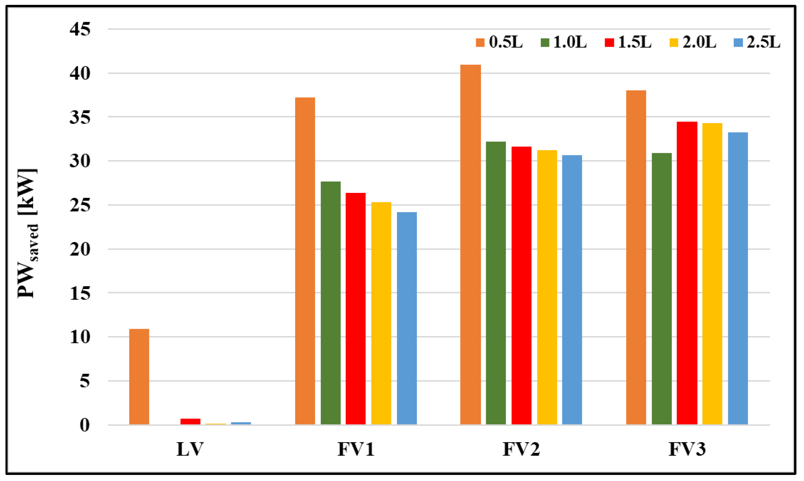
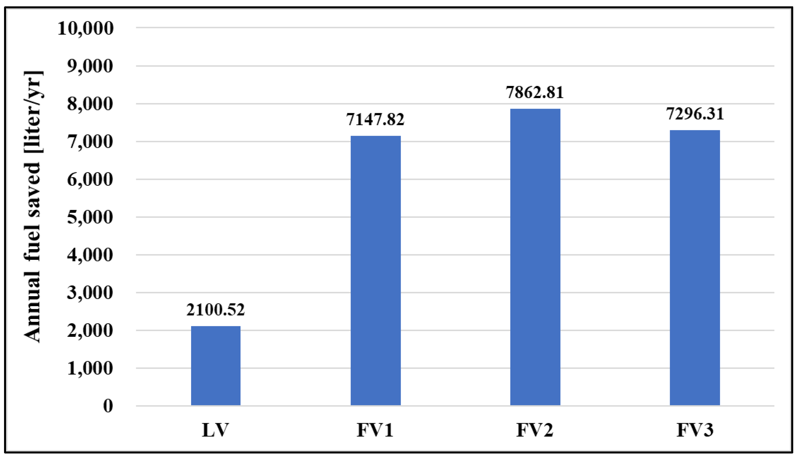
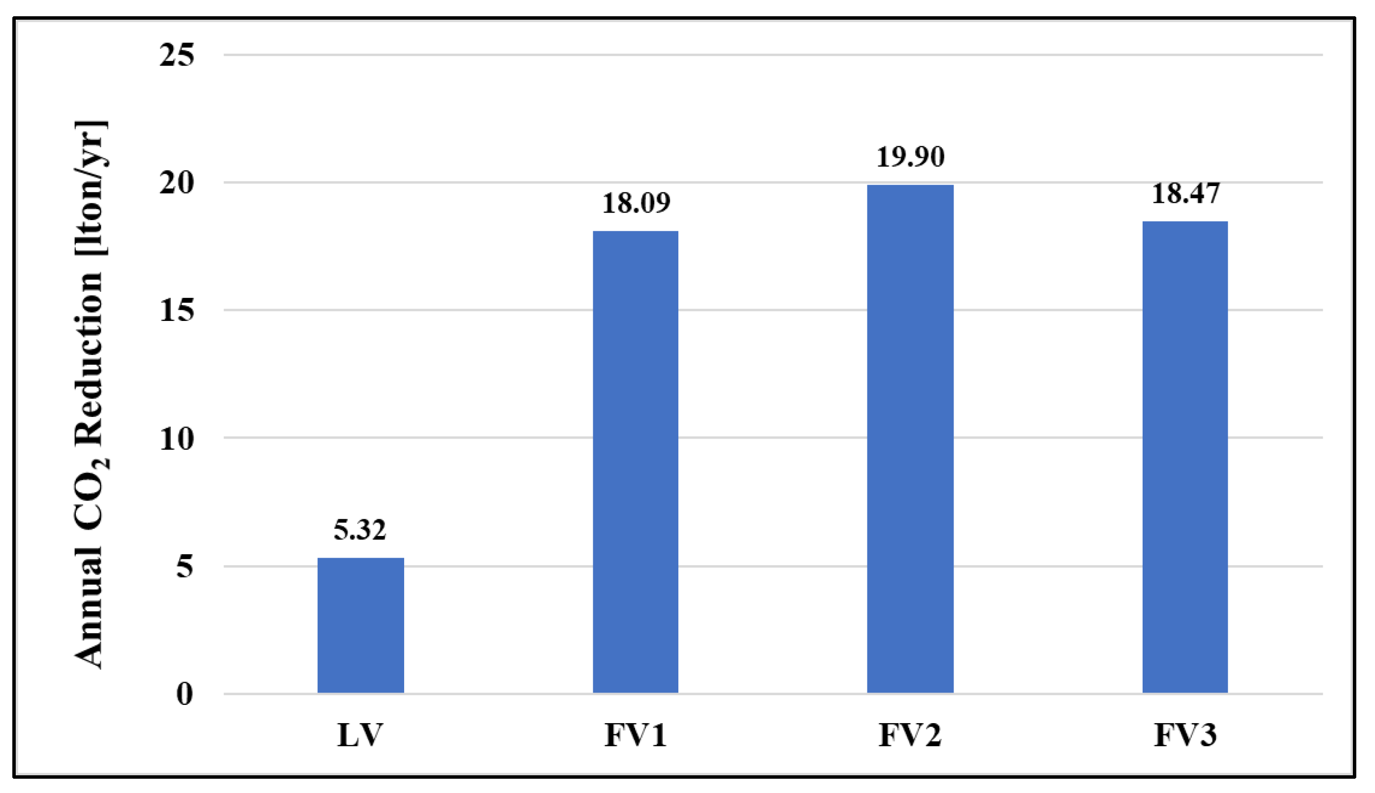
4.2. Fuel Efficiency and GHG Emission Improvement in the Model Vehicles

According to the research reports from the EU FT7 (SARTRE project, 2016), it was found that close distance between the vehicles in platooning improves the fuel efficiency for all vehicles [24]. In the case of a 6 m gap, which is half-length of the model HDV, the LV saved 8% of fuel compared to SV and up to 16% for the following FV [25]. We also predicted fuel consumption and GHG reduction in this study.

Figure 9 shows the tractive power saved by the vehicles platooning compared to the single moving vehicle (SV). For the leading vehicle (LV), the power energy was not saved much compared to SV but from the 2nd vehicle (FV1, FV2, FV3) the tractive power distinctively decreased. The power saved on the model vehicles platooning versus SV was calculated with Equation (7).

LV saved approximately 10 kW of power at the 0.5 L gap condition. Under 1.0 L~2.5 L gap conditions, a relatively narrower gap does result in a better traction power reduction than SV, and the power saved increases as the location of the model vehicle is far from the leading position. When the HDV’s gap is 0.5 L, the averaged traction power saved for FV1, FV2, and FV3 is 38 kW compared to the SV. Additionally, the FVs kept an average of 30 kW of power under the condition of the 1.0 L~2.5 L gap.

The fuel savings for each model vehicle platooning compared to SV was calculated with Equations (8)–(10).

The fuel consumption of SV by aerodynamic resistance was calculated as 5.2 km/liter at 100 km/h from Equation (10). When a single vehicle was moving, the fuel efficiency of FV1, FV2, and FV3 can be predicted as shown in

Table 4. Fuel mileage of each model vehicle platooning compared to the single moving vehicle (SV).

Vehicle’s Gap	Fuel Mileage [km/Liter]
	Single Moving	LV	FV1	FV2	FV3
0.5 L	5.2	6.1	10.7	11.9	10.9
1.0 L		5.2	8.4	9.3	9.0
1.5 L		5.2	8.2	9.2	9.9
2.0 L		5.2	8.0	9.1	9.8
2.5 L		5.2	7.8	9.0	9.6

. As a result, among simulation cases, the possibility of increasing the fuel efficiency of FV 1, 2, and 3 to 10 km/L is also confirmed under the 0.5 L conditions with maximum aerodynamic effects (100 km/h cruising driving condition).

According to KOTI (The Korea Transport Institute) report. 2021, Vol.62, the average daily driving distance of a loaded HDV was about 300 km/day in Korea for 2020 [26]. The averaged cruising speed of the HDV on a highway is 100 km/h; thus, the daily drive time is 3 h.

Based on HDV’s gap of 0.5 L, LV kept 2100 liter per year compared to SV. The saved result of an average of 7435 liter of FVs is shown in Figure 10. CO₂ reduction is calculated through Equation (11), resulting in LV saved by 5.3 tons per year and FVs saved by an average about 18.8 tons per year compared to the SV (Figure 11).

Thus, reducing drag force from the platoon can reduce the power required by the engine, resulting in reduced fuel consumption and GHG. Furthermore, aerodynamic drag is proportional to the square of vehicle speed, so high speed platooning could be more effective in saving energy.

5. Conclusions

This numerical study aimed to understand the aerodynamic effect of the heavy-duty vehicles platooning with the change in the platooning conditions; the gap between the model vehicles and the platooning position of the model vehicle. With the platooning condition change, aerodynamic resistance was analyzed to have the possibility of GHG emission reductions and fuel efficiency improvement. This study only considered steady driving conditions on a level road with no side wind. In addition, the aerodynamic characteristics of the vehicle were theoretically analyzed to determine the energy saving of the vehicle. Further study is needed to analyze the real driving state. From the research, the following were found:

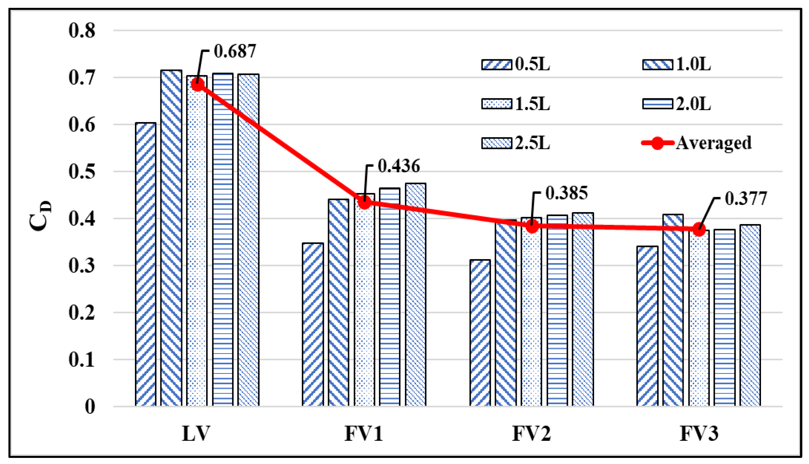
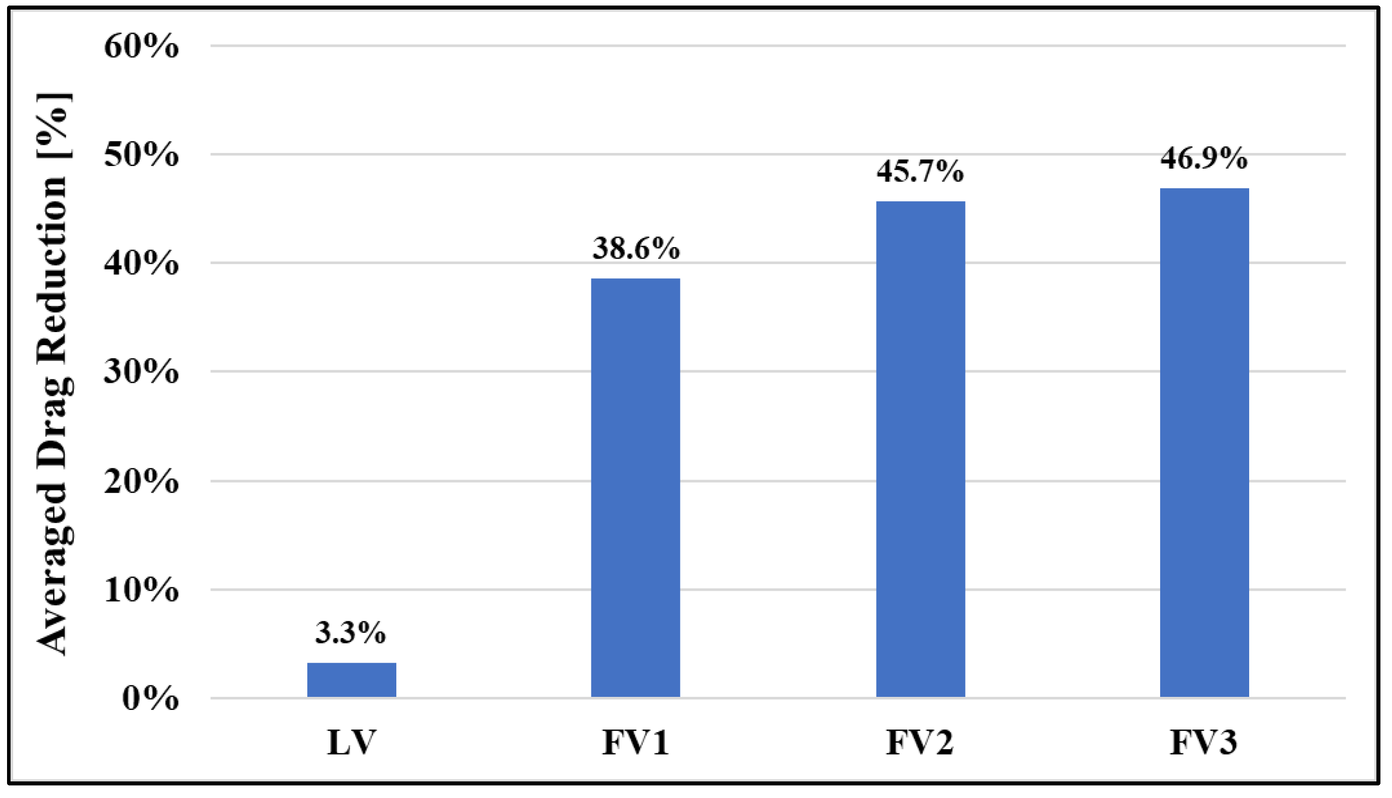
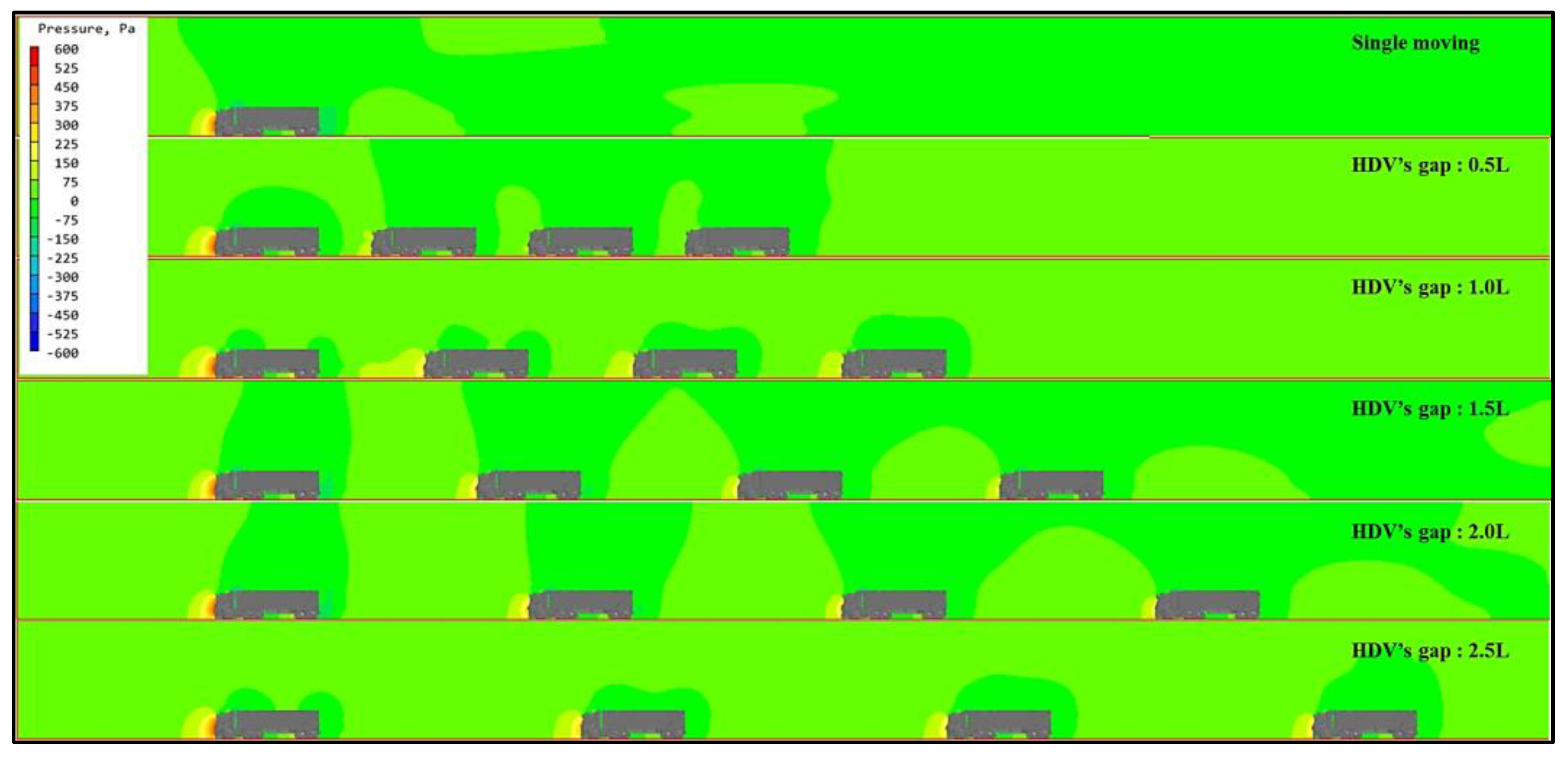
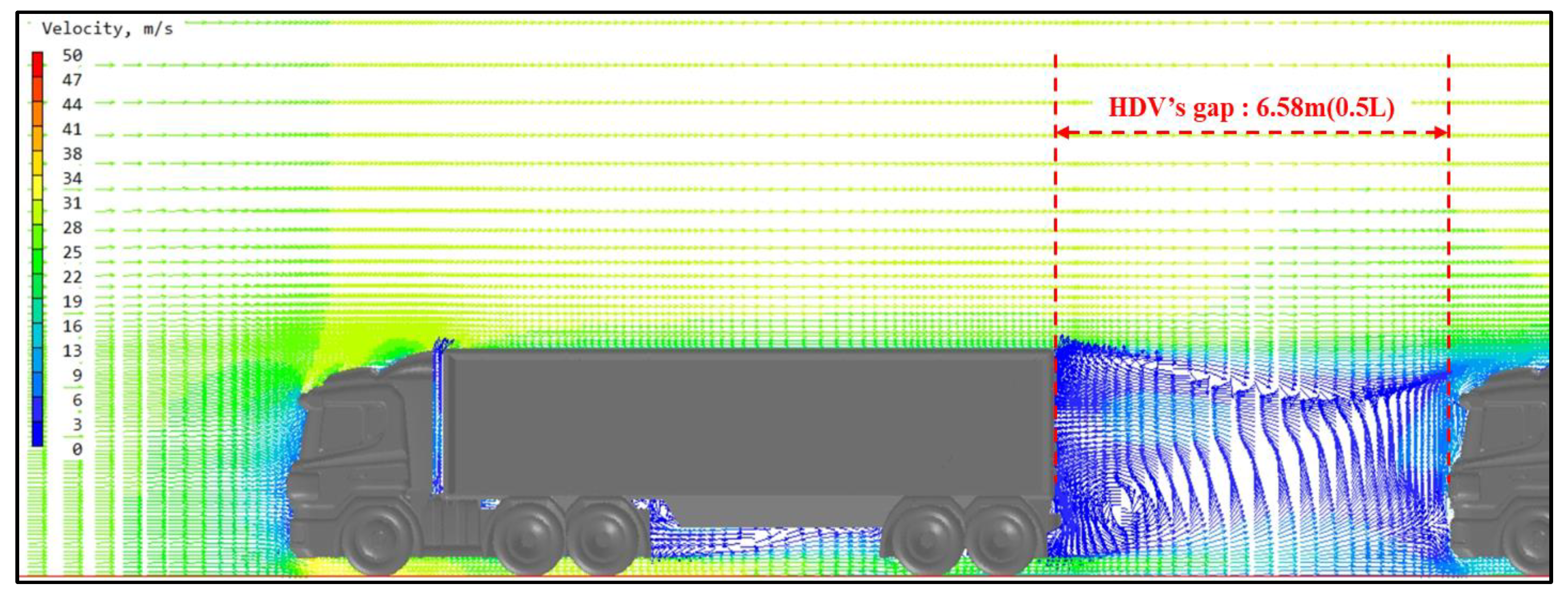
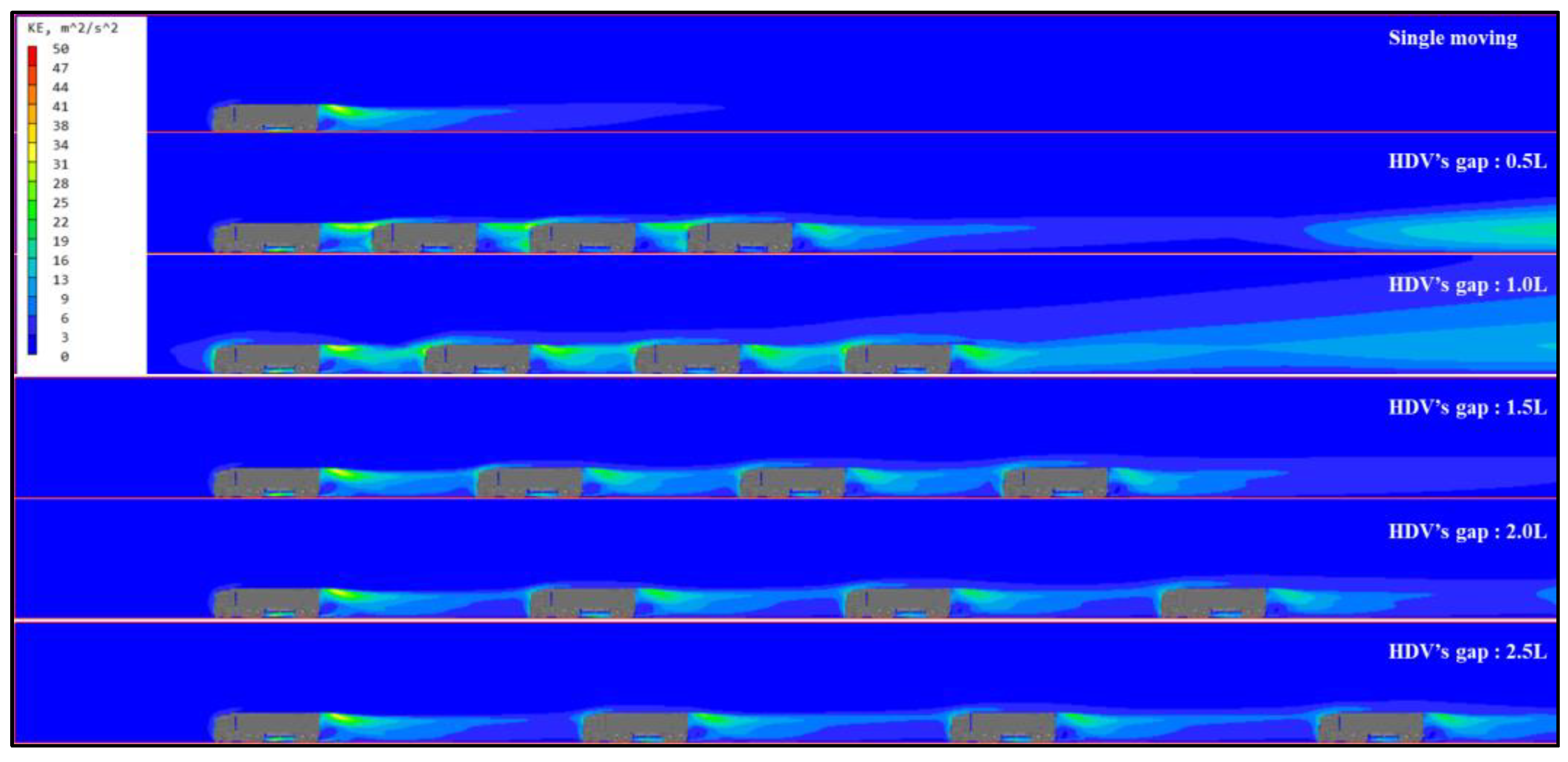
• The stagnation pressure of FV is reduced due to the rear vortex generated by the front leading vehicle. This is the main cause of the drag reduction on the FV. In this study, the drag of FVs was reduced over 50% compared to SV at the gap (0.5 L) (Table 3).
• The shorter the gap between the model vehicles platooning, the smaller C_D of FV, which indicates the shorter the gap distance, the more significant the influence of vortex on the FV. As the gap between the model vehicles widens, the rear vortex of the LV gradually decreases and the static pressure recovers to the ambient pressure. It is the reason for increasing the stagnation pressure of FV causing to C_D increase.
• Platoon driving has very positive effect not only to the fuel savings but also on the GHG reduction. Thus, the platoon driving mode of heavy-duty vehicles would seriously contribute to the logistics industry, economically and environmentally.
• This study hypothesized the driving conditions of autonomous vehicles based on V2X and suggested that the aerodynamic effect can be maximized when an appropriate platoon gap is set in vehicle-to-vehicle distance control. However, this study aimed to confirm the possibility of reducing GHG according to the platooning concept.
• This study performed a theoretical analysis using the FVM numerical simulation method. Platooning simulations were performed under the steady driving condition on a level road with no side wind to determine the fuel economy effect so this study might be used for reference. In future research, we will undertake the aerodynamic driving stability research on vehicle platooning. In the study, the weight of the vehicle with the road condition such as the friction coefficient and slippery factor of the road and the side wind, the gyration radius of the road with the tilted angle, etc., should be the important parameters to evaluate the road-load power for the study.

References

1. Buljac, A.; Džijan, I.; Korade, I.; Krizmanić, S.; Kozmar, H. Automobile aerodynamics influenced by airfoil-shaped rear wing. Int. J. Automot. Technol. 2016, 17, 377–385. [Google Scholar] [CrossRef] [Green Version]
2. Cihan, B. Numerical drag reduction of a ground vehicle by NACA2415 airfoil structured vortex generator and spoiler. Int. J. Automot. Technol. 2019, 20, 943–948. [Google Scholar] [CrossRef]
3. Song, K.S.; Kang, S.O.; Jun, S.O.; Park, H.I.; Kee, J.D.; Kim, K.H.; Lee, D.H. Aerodynamic design optimization of rear body shapes of a sedan for drag reduction. Int. J. Automot. Technol. 2012, 13, 905–914. [Google Scholar] [CrossRef]
4. Huluka, A.W.; Kim, C.H. A Numerical Analysis on Ducted Ahmed Model as a New Approach to Improve Aerodynamic Performance of Electric Vehicle. Int. J. Automot. Technol. 2021, 22, 291–299. [Google Scholar] [CrossRef]
5. Zhu, W.F.; Jiang, X.H.; Chen, X.; Lin, P.J. Automotive window seal design considering external aerodynamic load and surrogate constraint modeling. Int. J. Automot. Technol. 2016, 17, 853–864. [Google Scholar] [CrossRef]
6. Banks, J. Turbulence Modeling in PHOENICS. 2007. Available online: http://www.cham.co.uk/phoenics/d_polis/d_enc/turmod/enc_t342.htm (accessed on 13 June 2021).
7. Davila, A.; Nombela, M. Sartre-Safe Road Trains for the Environment Reducing Fuel Consumption through Lower Aerodynamic Drag Coefficient; SAE Technical Paper 2011-36-0060; SAE International: Warrendale, PA, USA, 2011. [Google Scholar]
8. Sun, X.; Yin, Y. Behaviorally stable vehicle platooning for energy savings. Trans. Res. Part C Emerg. Technol. 2019, 99, 37–52. [Google Scholar] [CrossRef]
9. Ministry of Land, Infrastructure and Transport. Development of Operation Technology for V2X Truck Platooning. Land Infrastructure and Transport R&D Report; 20TLRP-B147674-03; Ministry of Land, Infrastructure and Transport: Sejong, Korea, 2018.
10. Shin, K.; Choi, J.; Huh, K. Adaptive cruise controller design without the transitional strategy. Int. J. Automot. Technol. 2020, 21, 675–683. [Google Scholar] [CrossRef]
11. Emirler, M.T.; Guvenc, L.; Guvenc, B.A. Design and evaluation of robust cooperative adaptive cruise control systems in parameter space. Int. J. Automot. Technol. 2018, 19, 359–367. [Google Scholar] [CrossRef]
12. Saleem, A.; Al Maashri, A.; Al-Rahbi, M.A.; Awadallah, M.; Bourdoucen, H. Cooperative cruise controller for homogeneous and heterogeneous vehicle platoon system. Int. J. Automot. Technol. 2019, 20, 1131–1143. [Google Scholar] [CrossRef]
13. Wi, H.; Park, H.; Hong, D. Model predictive longitudinal control for heavy-duty vehicle platoon using lead vehicle pedal information. Int. J. Automot. Technol. 2019, 21, 563–569. [Google Scholar] [CrossRef]
14. Kang, Y.; Hedrick, J. Emergency braking control of a platoon using string stable controller. Int. J. Automot. Technol. 2004, 5, 89–94. [Google Scholar]
15. Alam, A.; Gattami, A.; Johansson, K.H. An experimental study on the fuel reduction potential of heavy duty vehicle platooning. In Proceedings of the 13th International IEEE Conference on Intelligent Transportation Systems, Funchal, Portugal, 19–22 September 2010; pp. 19–22. [Google Scholar]
16. Liang, K.-Y.; Martensson, J.; Johansson, K.H. Heavy-Duty Vehicle Platoon Formation for Fuel Efficiency. IEEE Trans. Intell. Transp. Syst. 2015, 17, 1051–1061. [Google Scholar] [CrossRef]
17. Ludwig, J. Concentration Heat and Momentum Limited; CHAM Technical Report TR326; POLIS, Phoenics On-line Information System: London, UK, 2008. [Google Scholar]
18. Chen, Y.-S.; Kim, S.-W. Computation of Turbulent Flows Using an Extended K-Epsilon Turbulence Closure Interim Report; No. NAS 1.26: 179204; NASA: Huntsville, AL, USA, 1987.
19. Kim, C.H. A streamline design of a high-speed coach for fuel savings and reduction of carbon dioxide. Int. J. Automot. Eng. 2011, 2, 101–107. [Google Scholar] [CrossRef] [Green Version]
20. World Nuclear Association. Heat Values of Various Fuels. Available online: http://www.world-nuclear.org/information-library/facts-and-figures/heat-values-of-various-fuels.aspx (accessed on 15 August 2021).
21. K-Petro (Korea Petroleum Quality & Distribution Authority). Quality Standard Chart according to Laws. Available online: https://www.kpetro.or.kr/eng/lay1/S210T239C379/contents.do (accessed on 15 August 2021).
22. Suppes, G.J.; Storvick, T.S. Sustainable Power Technologies and Infrastructure: Energy Sustainability and Prosperity in a Time of Climate Change; Academic Press: Cambridge, MA, USA, 2015; Chapter 5. [Google Scholar]
23. Guendehou, S.; Koch, M.; Hockstad, L.; Pipatti, R.; Yamada, M. Draft 2006 IPCC Guidelines for National Greenhouse Gas Inventories; Institute for Global Environmental Strategies: Hayama, Japan, 2006; Chapter 5. [Google Scholar]
24. Davila, A.; del Pozo, E.; Aramburu, E.; Freixax, A. Environmental Benefits of Vehicle Platooning; 2013-26-0142; SAE International: Warrendale, PA, USA, 2013. [Google Scholar]
25. Chan, E. SARTRE automated platooning vehicles. In Towards Innovative Freight and Logistics; Wiley: Hoboken, NJ, USA, 2016; Volume 2, pp. 137–150. [Google Scholar]
26. KOTI (The Korea Transport Institute). Report 62. 2021. Available online: https://www.koti.re.kr/user/bbs/BD_selectBbs.do?q_bbsCode=1093&q_bbscttSn=20210726174721314 (accessed on 20 August 2021).
Figure 1. A perspective view of the simplified model vehicle with its dimensions.
Energies 15 04390 g001
Figure 2. Numerical domain with the model heavy-duty vehicles platooning.
Energies 15 04390 g002
Figure 3. A typical numerical grid with the four model vehicles in platooning (658 × 99 × 87).
Energies 15 04390 g003
Figure 4. Variation in drag coefficient (CD) of each model vehicle in platooning with the change in the gap.
Energies 15 04390 g004
Figure 5. Reduction in the averaged CD of each vehicle in platooning compared to SV.
Energies 15 04390 g005
Figure 6. Comparison of the static pressure distribution with the change in the gap at 100 km/h.
Energies 15 04390 g006
Figure 7. Vortex generated in between LV and FV1 at 0.5 L and 100 km/h in speed.
Energies 15 04390 g007
Figure 8. Comparison of the turbulent kinetic energy distribution with the change in the gap at 100 km/h.
Energies 15 04390 g008
Figure 9. Tractive power (PWsaved) saved on the vehicles platooning compared to SV at 100 km/h.
Energies 15 04390 g009
Figure 10. Annual fuel saving on the model vehicles platooning compared to the single moving vehicle (SV) at a 0.5 L gap.
Energies 15 04390 g010
Figure 11. Annual CO2 reduction in platooning vehicle driving compared to the single moving vehicle (SV) at a 0.5 L gap.
Energies 15 04390 g011