Asset Profitability in the Electricity Sector: An Iterative Approach in a Linear Optimization Model

Abstract

In a competitive electricity market, generation capacities can exactly cover their full costs. However, the real market deviates from this ideal in some aspects. One is the concern of non-existent or insufficient scarcity prices. We present an iterative method in a linear optimization model to investigate the profitability of assets in the absence of scarcity prices and how the system changes when this risk is incorporated into investors’ expectations. Therefore, we use a two-step optimization of capacity planning and unit commitment. Iteratively, mark-ups at the height of uncovered costs are added to investment costs. This typically leads to a system with better investment profitability while keeping the system cost increase low. The methodology is applied to a simplified brownfield generation system, targeting CO₂-free power generation within 25 years. In a model with annual foresight of actors, iterations result in a generation system with significantly lower (or even no) uncovered costs for new investments within ten or fewer iterations. Our example case with full foresight shows that early-added gas (combined cycle) and wind onshore capacities are able to recover their full costs over a lifetime, even without scarcity prices. However, the contribution margin gap remains high, especially for storage and biomass.

1. Introduction and Relevance

Electricity generation as part of the energy system plays a key role in the way to a greenhouse gas (GHG)-neutral energy system. Although significant reductions have already been achieved in this sector in recent years, there is still significant transformation needed to achieve GHG-neutral electricity production. Therefore, for example, many countries have lately decided to phase out their coal-fired electricity generation. However, it is already becoming apparent that the decarbonisation of the transport and heat sectors will be accompanied by the increasing use of electricity as final energy in these sectors, resulting in a higher demand for electricity. At the same time, national targets and international commitments regarding GHG-emission reductions are steadily tightened and pulled forward, leading to a high pressure for an extremely rapid transformation of energy systems. Those aspects in combination require the electricity generation to reach carbon neutrality (or even net negative emissions) within a very short timeframe.

Studies on how the transformation of the power system can succeed are often calculated with optimization models (ref. [1], examples in [2,3,4]). With this modelling, a solution is found to how the demand for electricity can be met at a minimum system cost while complying with various technical and economic restrictions. Existing assets (In the following, we use the term “asset” to refer to all capacities that contribute to meeting the electricity demand, thus including conventional power plants, renewable power plants, storage and demand response technologies.) are usually considered assuming a remaining technical lifetime. To ensure that the demand for electricity can still be met when the capacity of existing assets decreases, the model has the option of deciding on the addition of new generation technologies as the integrated option for cost minimisation. The results outline the technology mix that can fulfil the corresponding power supply task at a minimum cost. The results of these model calculations serve as a basis for political decisions, e.g., with regard to support schemes, subsidies, guaranteeing the security of supply and grid planning, but also as a control mechanism for how, whether and at what cost political goals can be achieved. From this point of view, the application of cost minimisation approaches to this task is advantageous as it shows a normative transformation path.

However, in reality, there is a certain risk that the capacity additions identified by such a cost-minimising approach do not take place as calculated due to non-profitability in reality. This means that the addition of a certain technology may represent the solution with the lowest system costs from an economic perspective, but no investor would actually decide on this investment, as it is not profitable from an individual investor perspective.

According to economic theory for competitive energy markets (compare e.g., ref. [5], (p. 53)), all technologies can cover exactly their full costs ([5] (p. 123)), and cost-minimising modelling approaches basically follow these assumptions. However, this conclusion is only true if all conditions of perfect competition are satisfied. For example, scarcity prices (i.e., prices above the marginal costs of the most expensive technology) are required to occur at a sufficient level. For this to happen, there must be at least a few hours of scarcity in which the pivotal supplier is able to enforce prices above its marginal costs. In a market with overcapacities, scarcity prices are not possible according to economic theory, because at prices above the marginal costs, a producer would always be found who would offer at lower prices. However, scarcity prices at levels that would be expected under that theory have not been observed in existing European electricity markets (for explanations see Section 2) in the recent past. Furthermore, there is a risk that, even if scarcity exists, price spikes are limited (e.g., for political reasons), thereby preventing sufficient scarcity prices. These two aspects increase the risk for investors that sufficient scarcity prices to refinance the full cost of an investment will not occur in real markets. Accordingly, there is a risk that rational actors will not choose to invest in a particular technology even though it has been identified as the least-cost option in the cost minimisation model.

The existence of this risk has also been addressed in the latest description of the European Resource Adequacy Assessment (ERAA) methodology [6], which is the basis for the central pan-European assessment of the security of supply. The methodological approach to evaluating the economic viability of generation capacity is called Economic Viability Assessment (EVA), and the first results have already been published (see Section 3.3 for details).

From an investor’s perspective, however, the risk of missing scarcity prices does not necessarily mean that no investment will take place, but rather that they will apply a different or higher risk premium when calculating their investment [7,8]. Risk premiums can be included in optimization models as part of the investment cost. Technologies that must cover a higher proportion of their fixed costs through scarcity prices in order to be profitable will have to apply a higher risk premium than technologies that depend only slightly on scarcity prices, according to this logic. This, in turn, shifts the relationship between the investment costs of different generation technologies, and the model will find a different solution considering this new information. To implement this logic into model analysis, we propose an iterative modelling approach in this paper that captures exactly this relationship by gradually adding a risk premium to the assumed investment cost for the risk of an unprofitable investment (due to a lack of scarcity prices). On the one hand, this iterative methodology better reflects the decision behaviour of investors. On the other hand, the methodology leads to a system with lower uncovered costs while keeping the increase in system costs as low as possible at the same time.

The result does not necessarily correspond to a technology mix in which all technologies are actually profitable, but the result is a technology mix in which the calculated investments actually take place with a higher probability. The disadvantage of system-cost-optimizing modelling discussed above can thus be mitigated.

We apply the methodology described (and explained in detail in Section 4.1) in this paper as a highly simplified brownfield model for the German power sector and show how and why this changes the technologies chosen by the model. However, we describe the methodology in a general manner so that it is applicable to other models, for different regional areas and other scenarios.

Summarizing the above means that successfully managing the extremely rapid change in the electricity sector requires extensive modelling exercises to support policy decisions. In this paper, we aim to add one aspect to these results that has been little considered so far, as follows: We study the impact of the risk of insufficient scarcity pricing in real markets on the composition of technology choice and the profitability of individual technologies. This might be of special importance with regard to the question of whether insufficient scarcity pricing might inhibit required capacity investments on the way to a purely renewable-based electricity sector. The research gap we aim to fill consists mainly of the following two aspects: First, there are very few studies on the electricity sector that consider a model endogenous feedback loop between the risk of non-profitability and technology choice. Second, existing studies often examine profitability in a general manner, which does not allow one to distinguish between effects that stem from a simplified representation of reality in the model and effects from actual structural deficits in the real market. In contrast, we only focus on the effect of insufficient scarcity pricing on profitability, which allows for a clear cause-effect analysis.

With those two aspects, we contribute to improving the representation of non-optimality in electricity market modelling [9] and demonstrate a method on how to investigate one aspect of uncertainty for investors, which is often considered underrepresented in energy system models [10,11].

The paper is organised as follows: In Section 2, the theory of pricing in electricity markets and the formation of prices in linear optimization models are summarized. The approach chosen in this paper to account for profitability is explained and compared to existing modelling approaches to profitability. In Section 3, the model and data used are described as well as the details of the iterative methodology applied. The results before and after the iterations as well as under a myopic and a perfect foresight model approach are summarised in Section 5. Conclusions and recommendations for further development of this approach are drawn in Section 6.

The basic setup of model assumptions in this paper is based on key data from the German electricity sector, which is why Germany is also frequently taken as an example within the next sections.

2. Empirical Findings on Electricity Price Formation, Profitability and Investment in Competitive Markets

According to economic theory, the price in a competitive market is determined by the intersection of the demand and supply curves. Within a competitive electricity market, this usually means that the price for electricity equals the marginal cost of the supplier with the highest marginal cost that is in operation at a certain point in time [5] (p. 62). The term “usually” indicates that there are circumstances in which this is not the case. One is that prices can rise above marginal cost in times of scarcity of supply. In order to understand why this is necessary for an efficient market, it is useful to distinguish between a short-term market equilibrium and a long-term one [5] (p. 56). In a short-term market equilibrium, a generator will decide to generate output as soon as the market price rises above its marginal cost. In a long-term equilibrium, a generator needs to be able to recover its full costs (variable costs plus fixed costs); otherwise, it will decide to exit the market [12] (p. 13). Generators can gain revenue to cover their fixed costs from (non-scarcity) inframarginal rents, which is the delta between their own marginal cost and the marginal cost of the price-setting generator. However, if this were the only revenue, it would mean that the generator with the highest marginal cost would cover its variable costs only and would have no chance to recover any of its fixed costs. In combination with scarcity on the supply side, the generator will be able to set the price above its marginal costs in times of high demand as there is a chance that it will be pivotal (i.e., the generator is the only one being able to increase production anymore). This delta between the resulting market price and the highest marginal cost is called scarcity rent (compare [5] (p. 71)) and will, according to theory, be set at a level where the generator with the highest marginal cost recovers exactly its fixed costs. Higher prices than that would attract other investors to enter the market and thus cause prices to decline. This, in turn, means that the scarcity premium will settle at an optimum level in the long term. In such a long-term market equilibrium, all generators are able to recover exactly their fixed costs [5] (p. 123). A generator’s total earnings to cover its fixed costs (sometimes also called short-term profit or contribution margin) therefore constitutes from its inframarginal rent $r_{inf}$ (which equals zero for the generator with the highest marginal cost) plus a scarcity rent $r_{sc}$as expressed in Equation (1).

$$CM=r_{inf}+r_{sc}$$

(1)

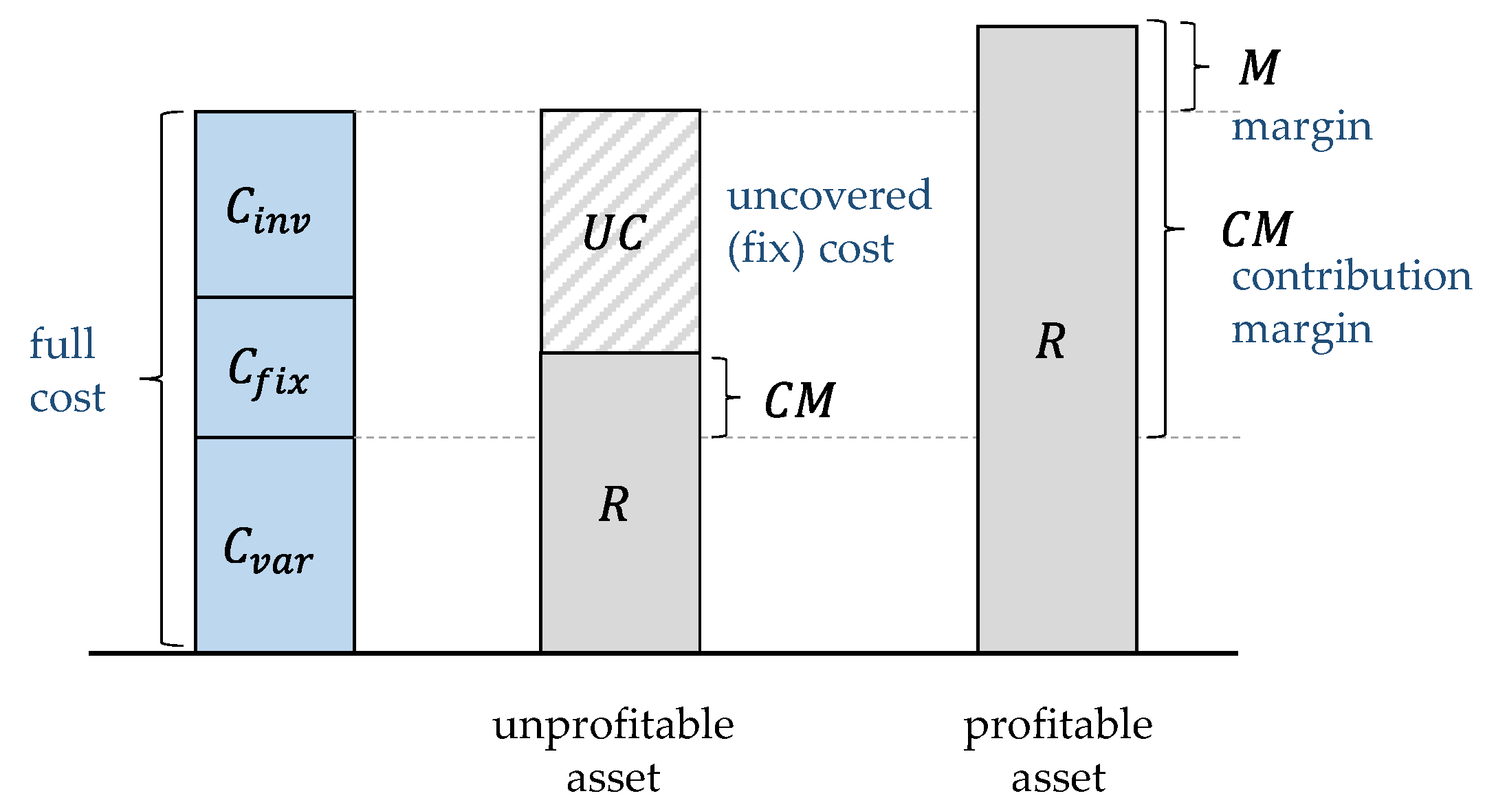
Furthermore, literature often distinguishes between the contribution margin (CM) reflecting the delta between revenue R and variable cost (Equation (2)). The second one is the (unadjusted) margin M which takes fixed operating costs and investment into account and therefore represents the delta between revenues and a generator’s full cost as in Equation (3). As we focus on new investments in this paper, it is crucial for an investor that he can expect a positive (unadjusted) margin M, otherwise, it is quite clear that he will not be able to gain any profit. Therefore, the unadjusted margin is the most relevant indicator for this purpose, and we use the term “margin” synonymously to M, while the term “contribution margin” is used for the term CM. An overview of the interrelations of these terms is also given in Figure 1 (see ref. [12], p. 14 for a more detailed breakdown of costs).

$$CM=R-C_{var}$$

(2)

$$M=R-C_{var}-C_{fix}-C_{inv}$$

(3)

As mentioned above, in an efficient competitive electricity market in its long-term equilibrium the margin M will equal zero for all generators. However, some aspects bear the risk that this situation will not materialize in a real electricity market. The case that prices in a real electricity market might not be high enough to recover investment costs is called the missing money problem [7]. This phenomenon can lead to a situation where the market fails to attract sufficient investments for serving the electricity demand.

Ref. [7] shows evidence that this problem actually occurs in the US liberalized electricity markets. The reasons why the missing money problem occurs are discussed in the following publications: Ref. [5] states that it is likely that there are old generators (not retired) in the system with higher marginal cost than the one operating, which means that the system actually is not scarce and scarcity rents might not occur or not be sufficient. Another reason frequently mentioned is that the majority of electricity consumers do not see real-time prices nor are able to adjust their electricity consumption to price signals, resulting in a high inelasticity of demand. A steep demand curve can support the emergence of price peaks, but in extreme cases, it can also lead to a situation where no market-clearing price can be found at all [13,14]. To avoid this situation, electricity markets often define a price cap that is applied when no clearing price can be found through the market. Whether and how high this price cap is set is a question of individual market design. A price cap that is set too low entails the risk of insufficient refinancing of capacities that need precisely these high prices in scarcity situations to cover their fixed costs. However, even in markets with non-capped prices, such as the German electricity market [15], there is a lack of empirical evidence that sufficiently high price peaks actually occur. Therefore, neither the question of whether sufficient price peaks occur in existing market designs nor the question of whether high prices—if they occur—are also “sustained” long enough from the political side, can be answered empirically.

The discussion about these real-world inefficiencies shows that there is a risk of retained investment in new power generation capacity, although—according to theory—the market is able to ensure the addition of enough capacity to achieve a sufficient level of security of supply. In the case of the German electricity market, this issue was analysed in detail in publications from 2011 to 2013 against the background of the question of whether or not Germany should establish a capacity market. The conclusion from this discussion was that the above-mentioned reasons are not sufficient to legitimize the introduction of a capacity market. On the one hand, it was argued that these inefficiencies either have very little impact or can be addressed by a careful market design. On the other hand, it was also highlighted that there was overcapacity in the German market at that time, leading to a fundamentally high level of security of supply (compare [8,16,17,18]). However, it is not the aim of that paper to add to this discussion, but the discussion provides evidence that there is some risk that the required investments might not occur. Instead, the procedure introduced in this paper offers an opportunity, to include this risk into the analysis of capacity development in a market-based power system.

An analysis of historical day-ahead electricity prices also indicates that there is still more generation capacity in Germany today than would be necessary to cover the peak load.

Table 1. Frequency of day-ahead prices above 100 EUR/MWh within the German/Luxembourg bidding zone (incl. Austria until 30 September 2018).

Price Range	2015	2016	2017	2018	2019	2020	2021
[100;200)	0	1	61	13	7	24	1306
[200;300)	0	0	0	0	0	1	156
[300;400)	0	0	0	0	0	0	9
[400;500)	0	0	0	0	0	0	1

shows the distribution of hourly prices in the German/Luxembourg bidding zone for the period January 2015 to October 2021 [19]. Although the maximum electricity price increased in the past years and the frequency of electricity prices >EUR 100 increased especially in 2021, maximum prices did not come close to investment costs of a peak load technology (investment costs for an open cycle gas turbine add up to around 57,000 EUR/MW with our assumptions s, compare

Table A1. Technical and economic assumption for generation technologies in CEM and UCM.

Technology	Emission Factor [t/MWhth]	Fuel Cost [EUR/MWh]th	Investment Cost [EUR/kW]	Variable O&M Cost [EUR/MWhel]	Fix O&M Cost [EUR/kW]	Efficiency [%]	Full Load Hours [h]	Lifetime [a]
Biomass (exist)	-	55.07		7.7	53	33	-
Biomass (new)	-	55.07	3300	7.7	53	38	-	30
Nuclear (exist)	-	6.28		9	102	33	-
Hard Coal (exist)	0.341	9.42		3.3	38	37.5	-
Lignite (exist)	0.364	8.22		3.3	46	37.5	-
Natural Gas OC (exist)	0.202	22.33		1.6	13	35	-
Natural Gas OC (new)	0.202	22.33	400	1.6	13	40	-	25
Natural Gas CC (exist)	0.202	22.33		1.6	24	44	-	30
Natural Gas CC (new)	0.202	22.33	700	1.6	24	60	-	30
PV (exist)	-	-		-	15	100	1105
PV. open area (new)	-	-	780	-	15	100	1105	25
Wind Onshore (exist)	-	-		-	13	100	2500
Wind Onshore (new)	-	-	1113	-	13	100	2500	25
Wind Offshore (exist)	-	-		-	93	100	3600
Wind Offshore (new)	-	-	2590	-	93	100	3600	25
Runriver (exist)	-	-		2.5	45	100	-
Others (exist)	0.267	31.49		2	12	35	-
Pumped Storage (exist)	-	-		0	12	73.5	-
Pumped Storage (new)	-	-	1218	-	12	76	-	100
Stationary Batteries (new)	-	-	550	-	20	90	-	15

.) or an estimated value of lost load in the whole period considered (estimates of the value of lost load show a very wide range in literature, summarised e.g., by [20] between 1500 EUR/MWh and 22,940 EUR/MWh.).

The fact that overcapacities exist not only in Germany but also in other European countries is also shown by [21]. Therefore, at least in the medium term, there seems a risk that there will be no scarcity prices in the German but also in other European electricity markets, which would be necessary to refinance the investment costs of new assets and to cover the fixed costs of existing assets. In recent years, for example, it has been observed that existing gas-fired power plants in some countries have actually become unprofitable [22]. Ref. [23] even concludes that “virtually all generators encounter a revenue gap in the current energy-only market”.

Another reason for the missing money problem can be that compensation for ancillary services and/or reserve provisions are insufficient [24]. Some sources also mention the volatility of electricity prices as a potential risk for insufficient investment, which will become even more serious with the increasing share of variable renewable energies (VRE) (discussion in [25]). However, e.g., ref. [8] states that price volatility alone does not constitute a market failure, but the impossibility to hedge against those risks might do so. Ref. [24] calls this issue the “missing market problem” and points out that missing markets might lead to insufficient investments, meaning that an investor is not able to adequately use forward or future markets for hedging its risks. This is particularly relevant considering that the usual refinancing period of a generation capacity is long and changes in political targets and/or reforms are likely to occur within this period.

Therefore, there are plenty of empirical indications for a certain risk that scarcity prices either will not occur or will not occur sufficiently to refinance fixed costs. In the medium term, this probably results from existing overcapacity; in the long term, it may be compounded by the risk of price caps or other reasons hampering the occurrence of sufficient price peaks in the market. Investors assessing the risk of a new investment today must take this fact into account in their deliberations. While this does not necessarily mean that there will be no capacity additions at all, investors would likely take the risk of a shortfall into account in the form of a risk premium. This would de facto increase investment costs and lead to a correspondingly lower level of investment (compare also [8]). Technologies that are heavily dependent on scarcity prices for their refinancing would assume a proportionally higher risk premium than those that can already cover a large part of their fixed costs through inframarginal rents. Accordingly, the ratio of investment costs between the technologies will also shift, leading to a different composition of the optimal technology mix.

3. Modelling of Pricing and Profitability in Linear Optimization Models

In the following chapter, we address the link between the empirical findings above and the price formation in an optimization model in Section 3.1. We then present our approach to considering asset profitability in a schematic overview along with a discussion of its real-market interpretation. With this background, we can contrast our approach to existing literature, thereby discussing the WACC principle, discount rates, endogenous and exogenous profitability calculations, the methodology of the latest European resource adequacy studies, as well as the link to publications in the area of so-called modelling to generate alternatives. Chapter 3 concludes with a summary of the strengths of the applied modelling approach and the methodologic rationale why we apply the approach to a myopic as well as a perfect foresight model.

3.1. Prices and Cost in a Linear Optimization Model

As the pricing mechanisms in competitive electricity markets based on economic theory reflect the marginal cost of the most expensive generation unit required to meet the demand, electricity prices in linear optimization models can be read from the dual variable of the electricity demand equation (e.g., ref. [26]) (This applies at least to those models in their very basic configuration. Advanced electricity market models represent many characteristics of an electricity sector in detail, e.g., expansion or decommissioning targets are set, must-run conditions are set, minimum shares of renewables are exogenously specified or additional demands for heat, hydrogen, etc. are taken into account. All of these model features can ultimately influence the electricity price, so the simplified explanations of Section 2 alone are no longer sufficient to explain it, which is why we refer here to a highly simplified model only.). In our simple example, this implies that prices above marginal costs will occur in these models only if generation capacity is actually scarce. This could—for example—be the case in a capacity expansion model, where no existing assets are considered (often called “greenfield modelling”) or the available capacity of existing assets is not sufficient to cover demand at all times. In this case, the model is usually able to choose the cost-optimal generation mix out of several technology options and consequently, scarcity rents above marginal costs will be visible in the price structure and the missing money problem will not occur (e.g., ref. [27]). In a pure unit commitment model, on the other hand, the cost-optimal dispatch under sufficient capacity is found only, i.e., prices will not include scarcity rents but follow the generator’s marginal operation cost. With respect to the profitability of assets, this means that assets in a capacity expansion model earn exactly their full costs and that $r_{sc}>0$ and $M=0$ applies. In a pure unit commitment model, no scarcity rent occurs ($r_{sc}=0$) and thus $CM=0$ is valid for the technology with the highest marginal cost and $CM=R_{inf}>0$ for all other technologies. Furthermore $M\le 0$ applies to all technologies.

3.2. Considering Profitability Risk by an Iterative Modelling Approach

In this paper, we use a two-step procedure based on two linear optimization models, consisting of one model that optimises capacity expansion planning (and unit commitment at the same time) and one model that has no possibility for capacity additions but calculates only the dispatch of existing units. The models are called the capacity expansion model (CEM) and the unit commitment model (UCM) in the following. The models correspond with respect to all assumptions (costs, technology parameters, temporal and spatial resolution, etc.) and differ only in that the cost-optimal capacity mix calculated in the CEM is assumed as existing units in the UCM (see Figure 2). With this model setup, a cost-optimal capacity mix can be evaluated, but at the same time, a price series without scarcity rents are generated.

The objective function in both models corresponds to the minimisation of system costs, i.e., those costs to meet the exogenously specified electricity demand. In both models, the system costs include the variable costs for operation and maintenance (OaM), the fuel costs, carbon costs and the fixed OaM costs of all generation technologies. In addition, in the CEM, investment costs are also part of the objective function. To account for the different lifetimes of the generation technologies, investment costs are allocated to the respective technical lifetime by an annuity approach. As described in the previous sections, there is a certain risk for an investor that the occurrence of scarcity prices is not sufficient to refinance an investment. In our model setup, the uncovered costs UC of a technology t in year y represent the contribution margins at risk for investments in those new generation assets in case the market price does not exhibit any scarcity price peaks. For a myopic case, the uncovered cost $U{C}_{y,t}$ is defined by Equation (4), where A corresponds to the annuity of investment costs.

$$U{C}_{y,t}=r_{inf,t,y}-C_{fix, t,y}-A \left(C_{inv,t}\right)$$

(4)

Since uncovered costs represent a risk for a potential investor, we assume a mark-up on the investment costs of those technologies. The relation of the mark-ups thereby corresponds to the relation of the uncovered fixed costs. On the basis of these increased investment costs for those technologies, we restart the CEM, resulting in a different composition of the capacity mix than that of the first iteration. Since resulting prices in the UCM, and thus the profitability of technologies, change as a result, we apply this methodology iteratively and assume new mark-ups for the next CEM run. We continue these iterations until one of the termination criteria described in Section 4.1 is reached. The result is a capacity mix with higher system costs—since any change from the original optimum solution means obviously higher costs—but at the same time lower total uncovered costs. In addition, this capacity mix takes into account the technology-specific risk of uncovered fixed costs and the resulting shift between technologies.

Compared to the decision process of an investor, the mark-up on investment costs assumed in this way has similar effects on the model results as an increase in the weighted average cost of capital (WACC) or a technology-specific hurdle rate. However, it is not to be understood exactly as such and, due to the methodology described above, can be significantly higher than the WACC or hurdle rate normally assumed in the literature. The mark-up is rather a tool to obtain the model to find a solution that is system cost-optimal but at the same time minimises the sum of uncovered fixed costs. A mark-up on investment costs is particularly useful in this context because it can be deducted from the results ex-post. In addition, marginal generation costs are not affected, and thus neither are prices that follow marginal costs.

A different approach would be to assume mark-ups on the variable cost to the extent of uncovered cost from the previous iteration. This could have a similar impact on model results, namely, that technologies with high uncovered costs are used less in the next iteration. However, this procedure would affect marginal costs and thus prices in the UCM, which makes it more difficult to deduct the effects of this mark-up from the model results ex-post. Higher investment costs in turn influence the level of the scarcity premiums only, which are not considered in the profitability calculations. This methodology, therefore, offers a possibility to identify a capacity mix with very little intervention in the model results, which is system cost-optimal but at the same time has lower uncovered costs due to missing scarcity prices compared to the initial solution.

From an optimization point of view, this approach leads to a simultaneous minimisation of system costs and uncovered costs. Since electricity prices are not known endogenously within an optimization, the two components cannot be minimised simultaneously. To still find such a solution, the markup on the investment costs acts as a “penalty term” for the uncovered costs of the previous iteration, which leads to the fact that uncovered costs become part of the system costs and will thus be part of the minimisation.

As a result, technologies with high uncovered costs are used less, which has the following two effects: On the one hand, this results in lower uncovered costs since technologies with high uncovered costs are exchanged for technologies with lower uncovered costs. On the other hand, this also leads to shifts in the price duration curve, which can have a positive effect on margins and thus further reduce uncovered costs, but can also have a negative effect on contribution margins. Thus, there is no guarantee that this method will result in systems with lower uncovered costs in all cases (Although it cannot be proven that the iterative procedure will converge at anytime, we observed good convergence after a limited number of iterations in almost all cases (see Section 5.2).). The heuristic termination criteria ensure that the cases in which the negative effect on margins predominates are not considered any further. The specific effects of the markups on generation, prices and margins are illustrated by a simple example in Appendix B.

3.3. Other Modelling Approaches

The problem of uncertain profitability of investments in competitive power markets and within a cost-minimising approach is well known in the literature. There are several existing methodological approaches to considering profitability in energy-economic modelling.

A first and very convenient approach is to include the risk of profitability in discount rates and integrate those adjusted specific investment costs into cost minimisation models. There exists an extensive literature on the identification and selection of appropriate discount rates. For example, ref. [28] finds that social discount rates and technology-specific hurdle rates can strongly influence the energy system’s composition and behaviour. The authors of ref. [29] summarise social and individual discount rates used in studies and emphasise the importance of differentiating rates among different investor groups. The authors of ref. [30] propose actor- and region-specific discount rates to adequately reflect investor behaviour in optimization models, while [31] differentiate between sector- and actor-specific discount rates in their scenarios.

In summary, these calculations take into account different risks through corresponding premiums, but in the model calculation, it is implicitly assumed that these fixed costs can be fully covered. However, we see this as uncertain in real markets, as pointed out in Section 2. In contrast, our model setup generates an energy system in which (due to deviations from a perfectly competitive market) the fixed costs cannot be covered, and we examine the shifts in the energy system as a result in this particular example case by an iterative procedure.

Optimization models are also used to quantify asset or technology rents in defined scenarios, where the modelled electricity prices are used ex-post to calculate revenues. For example, rents on the asset level are examined under the influence of various policy measures in [32]. Ref. [33] calculates the shift in rents between generators and consumers also using a linear optimization model. In [34], the profitability of new and existing assets is calculated and evaluated with respect to the necessity of a capacity market. Although these approaches are able to quantify differences in profitability of different investments in competitive power markets, they do not model the impact of those differences on the development of the generation mix in the market. Ref. [35], for example, strives for that, as he implements a model endogenous consideration of profitability. However, the revenue calculation there is performed with an exogenously assumed subsidy and is therefore not completely modelled endogenously.

Ref. [36] applies a Monte Carlo simulation to determine the distribution of returns for different technologies. As he assumes invests and disinvests exogenously, no scarcity prices can be detected by this approach, and consequently, net present values (NPVs) for all technologies turn out to be negative. Ref. [25] conducts technology-specific risk measures from Monte Carlo simulations with a generic investment and dispatch model, thus considering investment decisions endogenously. However, the feedback effects on the investment decisions based on calculated profitability are not investigated in both cases.

The issue of profitability of generation capacities is currently also the subject of a discursive platform in the context of the major resource adequacy studies of the European network transmission system operators (entso-e). Following the Agency of the Cooperation of Energy Regulators (ACER) decision No 24/2020 [37], entso-e will implement a so-called economic viability assessment (EVA) as part of the European resource adequacy assessment, which evaluates market exits and entries based on an asset level comparison of revenue and costs. With a methodology still in the proof-of-concept stage, the EVA was first conducted within [38] and found significant capacity in Europe to be non-profitable (75 GW in 2025, revenues from capacity markets not considered). An iterative approach is applied in the latest adequacy study for Belgium [39] as follows: Revenues and costs arising from the dispatch simulation are used to calculate an internal rate of return on an asset level, which is compared to a technology-specific hurdle rate. Iteratively, the least profitable unit is then removed from the system and replaced by the most profitable out-of-market unit—until all units in the market are viable. This way, a non-viable gap of a maximum of 5.4 GW in Europe was found in 2025.

Obviously, the methodologies and results of these studies (still?) differ greatly. With this publication, we do not necessarily want to propose a new methodology for how to evaluate profitability in the frame of these studies. Rather, we want to place it in the theoretical framework and emphasise that in a long-term equilibrium, even under perfect competition, all producers can exactly cover their costs (see Section 2). Thus, a separate profitability calculation is necessary only for those aspects where the real market deviates from these assumptions. We consider these two issues of (1) the occurrence of sufficient scarcity prices and (2) the limited foresight of investors to be most relevant and therefore focus on the detailed analysis of their impact on profitability in the following.

From a methodological point of view, the paper can also be classified in the literature dealing with the so-called modelling to generate alternatives (MGA). The approach described here follows a similar idea to that of MGA, namely, not only to identify a single optimal solution but also to identify possible alternative solutions and thus take into account structural uncertainties that have not been modelled. In the MGA, the near-optimal solution space is systematically searched for solutions that show the smallest possible change in the objective function value but are maximally different with respect to the result variables [40]. The model structure is changed in an iterative process. In [41], among others, this approach is also applied in energy system modelling. Ref. [42] expands this method to identify all near-optimal solutions and ref. [43] proposes a method to determine “maximally different global energy system transition pathways”. The approach used here follows a similar idea but differs methodically from the following approaches: On the one hand, only a change of parameters is made between iterations and the model structure is kept identical. On the other hand, not all or maximally different solutions are systematically searched for, but solutions under the risk of insufficient scarcity prices are selectively identified.

The distinction of the methodology proposed here from existing approaches can be summarised as follows: Unlike several of the existing approaches to considering profitability in energy system modelling, the methodology proposed here follows an iterative procedure. This means, above all, that results not only provide a statement on whether an asset is profitable or not under given assumptions but also consider the feedback loop between risk of non-profitability and investments (and consequently the technology mix). In contrast to existing iterative approaches, we limit our research to exactly the following two possible reasons for non-profitability in order to clearly identify cause-effect relationships: namely, insufficient scarcity pricing and limited foresight of investors. The assumption of an existing non-optimal generation mix in our model runs (brownfield) adds another valuable aspect of real market conditions.

3.4. Myopic vs. Perfect Foresight

Model calculations for the transformation of the power system often consider a long-time horizon of several years or decades. Optimization can be performed over the entire period under consideration (perfect foresight), the years can be optimised separately (myopic), or an “intermediate” way can be selected in which several years are optimised simultaneously. The reduction of the optimization period is a possibility to reduce the computing time significantly [44]. This may be necessary because power sector scenarios often require a high level of detail in terms of spatial, temporal and technological resolution. However, a shorter optimization period also takes into account that, in reality, an actor does not have complete information about the development of all influencing variables over such a long time horizon. In particular, this also applies to the information available to an investor at the time of his investment decision. The investor always has to take his decision under uncertainty about future developments, especially about costs and revenue opportunities. Considering that, in reality, the investor has obtained some reliable assumptions about future developments for some of the next years, but at the same time, a decision on an investment in a generation asset takes some years until it is realised, the myopic approach becomes probably closer to reality. This is because it models the investment decision in a way that the decision-maker would have ideal information for a short time period in the future, corresponding to the period between investment decision and commissioning of the asset, but no information thereafter.

A model run with perfect foresight, therefore, overestimates the information that is actually available to an investor as a basis for decision-making. However, such model runs show other advantages, e.g., they provide information from a more central point of view on how a cost-optimal capacity mix will develop or how a GHG mitigation path at minimum costs over several years could look like. This result is a decent one as it represents the normative transformation path with the least cost. At the same time, it is clear that it will not be possible to achieve this path, as information about the future is not completely evident at the time of decision. However, this reasoning misconceives that, at the time of the analysis, information about the future relies on assumptions only and is in reality not known exactly. This means that the decent normative path would be normative in terms of least cost only if the theoretical case occurred that the assumptions were realised exactly as assumed, which will never be the case. This means that the advantage of drawing up a normative path is not as reasonable as it looks.

Due to that reasoning and the fact that a realistic future path can never be evaluated exactly due to uncertainties, we propose to evaluate both “extreme” assumptions to provide some idea to the decision maker about the uncertainties of the future. Therefore, we apply our methodology to both “extreme cases” (1-year myopic and perfect foresight over the entire modelling period) and compare the results.

In the myopic model approach, investment costs are assumed as an annuity over the depreciation period of a technology (described e.g., in [45]). Accordingly, the mark-up in the myopic calculation only relates to the number of uncovered costs of the respective year. Information on how revenues develop over a lifetime, or whether a technology (from a system-cost perspective) is decommissioned before the end of its lifetime, is therefore not included. In other words, we assume that the cost and revenue situation in the first year remains constant in all other years of the technical lifetime. As already mentioned, this represents—despite any consideration above—an “extreme” assumption with regard to the foresight of actors. Therefore, we contrast this solution with a perfect foresight calculation. Here, the mark-up on investment costs corresponds to uncovered costs incurred over the modelling period, i.e., it includes information on changing revenues or a possible early decommissioning (In the current phase of transformation, this aspect is very relevant, as follows: With the phase-out of coal-fired power generation, a significant proportion of controllable generation capacity is leaving the system in many electricity sectors. On the way to emission-free power generation, gas-fired power plants represent a bridging technology, as they are controllable but show a lower emission intensity. They can thus be an important building block for ensuring the security of supply on the way to a zero-emission power generation system, but can no longer be used in a fully decarbonized power generation system. The more the climate targets are tightened or the GHG neutrality targets are moved forward, the shorter the period in which these assets have the opportunity to refinance their full costs.).

4. Proposed Modelling Approach

4.1. Modelling Structure for Identification of Investment Premium

As shown in Figure 2, we determine the capacity mix in a capacity expansion model (CEM) and run a unit commitment model (UCM) subsequently in order to derive prices without scarcity rents in the first instance. Then, we calculate uncovered fixed costs per investable technology from the UCM result and assume a technology-specific mark-up on investment costs for the next iteration for each technology with negative margins (i.e., with uncovered fixed costs) only.

This iterative procedure in the myopic model—in which the iterations are performed separately for each year—is described in Figure 3 as a flowchart. After the two model runs with CEM and UCM, the uncovered fixed costs UC of each invested technology follow Equation (4). Original investment costs of iteration 0 are used to calculate UC, since the iteratively assumed mark-up here only serves as a “tool” to find a solution with lower uncovered fixed costs. The sum of uncovered costs across all technologies then serves as an indicator for the following two termination criteria of the iteration: (1) iterations are terminated if either the moving average of UC over two iterations increases twice in a row or (2) if the change of UC in two consecutive iterations is less than 0.001% of the original system cost. If none of the termination criteria is reached, an updated mark-up on investment costs of the previous iteration is assumed and the CEM is started again. If several iterations are required, the mark-up on investment costs will accumulate. If one of the two termination criteria is met, iterations are terminated for the year under consideration. The capacity mix of the last iteration is then assumed to be the existing capacity mix for the following year, and the iterations are continued identically for the following year—as well as for all other years considered.

In the case of a perfect foresight calculation, the procedure is identical, except for the sequential calculation of the years. Thus, the mark-up on investment costs does not correspond to the annual uncovered fixed costs but to those over the entire modelling period.

4.2. Model Description and Data Assumptions

The model used for the CEM and UCM runs is a very basic version of the European Electricity Market Model (E2M2). E2M2 is a bottom-up techno-economic model using linear or mixed-integer programming with the minimisation of power system costs as an objective function. For a more detailed description, basic model equations can be found in [46], recent extensions and applications, e.g., in [32,47,48,49]. The CEM optimises endogenous investment and dispatch simultaneously, while for the UCM run only dispatch is an endogenous decision. Electricity demand, emissions, fuel prices and the existing generation mix are linked to the key figures for the German electricity sector in 2020. However, E2M2 is applied in a very basic version for this work, which in concrete terms means that, e.g., heat production from combined heat and power, reserve provision, electricity exchange to neighbouring countries as well as startup and shutdown costs are not considered. In principle and depending on data availability, the approach and the model can consider these aspects as well, but since the focus of this paper is on the demonstration of the methodology and its implications, we keep the model as simple as possible.

However, we assume an existing generation mix with a simplified market exit curve (considering the German phase-out of nuclear and coal power plants) over the modelling time, which covers a 25-year period in 5-year steps. An upper bound for GHG emissions is set, declining linearly to zero until Y25. This model configuration is oriented towards the possible development of the German power sector with GHG neutrality in 2045, starting in 2020. However, considered years are denoted as Y0 to Y25 in the following to avoid the impression of a full-scale power sector analysis, which is not our intention in this paper. Support of renewables is considered for existing assets until the end of their funding period, while other technologies can be chosen endogenously by the CEM assuming their actual cost without further subsidies. Since prices are particularly important for the profitability of assets, we use an hourly time resolution in both models. Existing, as well as newly invested capacities, can be shut down before the end of their technical lifetime endogenously by the optimization if it serves cost minimisation.

In summary, the model set-up is a simplified brownfield calculation until 2045 with a high temporal resolution and based on the German electricity sector, in which no political subsidies are assumed for capacity additions. Market-exit for existing and invested assets follows an exogenous assumption but can be pulled forward for most technologies by endogenous divestment. Market entries are purely endogenous decisions.

The model configuration was chosen here, and thus exhibits the following deviations from the assumptions of perfect competition:

• No scarcity prices occur;
• The capacity mix is not in a long-term optimum (renewable existing assets cannot be disinvested);
• And there is a limited foresight of actors in the myopic case.

The validation of the coupling between CEM and UCM has confirmed that the two models give identical results in terms of generation quantities and hourly dispatch. The prices are also identical except for the scarcity prices in peak hours, which, according to the theory in Section 2, only occur in the CEM. The price duration curves from CEM and UCM are exemplarily shown for Y20 in Figure 4.

All technical and economic assumptions for existing and investable technologies in the two models are summarised in Appendix A (Table A1). The existing capacity mix consists of photovoltaic (PV), wind onshore and offshore, hard coal, lignite, natural gas combined cycle (CC), natural gas open cycle (OC), nuclear, biomass, run-of-river and pumped storage technologies. Other power plants are predominantly oil-fired and grouped under other (non-renewable). Investment technologies available to the model are natural gas OC and natural gas CC, PV, wind onshore and offshore, biomass, pumped storage and stationary batteries, each with no upper limits on investable capacity. Demand-side management (DSM) offering flexibility on the demand side is not taken into account for simplicity in this test case, as the inaccuracy is estimated to be too high if we assume an aggregation that is comparable to that of other technologies (however, DSM flexibility could be considered in the same way as other technologies in this approach). Emission factors for conventional fuels are taken from [50], fuel costs from [51], investment costs, fixed OaM costs and technical lifetimes from [2], variable OaM costs from [52], full load hours from [53] and biomass assumptions entirely from [54]. For an easier interpretation of the results, variable and fixed OaM costs are assumed to be identical for existing and new investments. However, the marginal costs of new investment are lower than those of an existing asset of the same technology due to higher efficiency. A technology-independent WACC of 10% is assumed for the annuity of the investment costs, based on [55].

Electricity demand and Y0 limitation of GHG emissions are consistent with historical levels in the German power sector in 2020 [56,57]. It is assumed that the power sector is to be completely decarbonized within 25 years; accordingly, an emission cap decreasing linearly to zero over the years is specified. All other costs and technical assumptions are assumed to be constant over the modelling period, i.e., there is no trend development.

The model assumptions as a whole contain some significant simplifications compared to reality. However, this serves to simplify the interpretation of the results and constitutes an acceptable step since the focus of this work is on the demonstration of the methodological approach and not on quantitative model results as a recommendation for decision-makers.

5. Results

In this chapter, the results of the myopic base model run (iteration 0) are presented and discussed first (Section 5.1). Changes in the myopic results due to iterations are then discussed in Section 5.2. The same follows for the results of the perfect foresight case in Section 5.3. Additionally, we have added a further simplified schematic example of the iterative methodology in Appendix B to demonstrate why and how the methodology used in this paper reduces the sum of uncovered fixed costs.

5.1. Model Results before Iterating (Myopic)

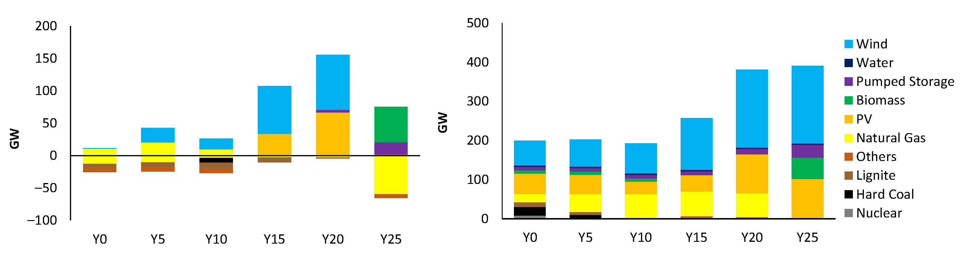
The results of the CEM for iteration 0 show that the capacity mix changes strongly from coal and lignite to gas capacities in the medium term due to model endogenous invest and decommissioning. In the long term, it shifts from gas to a system with a very high share of VRE, as well as storage and biomass capacities (see Figure 5, right) to achieve assumed GHG emission limits. In years Y0, Y5 and Y10, there is an addition of gas-fired CC power plants as well as wind onshore. At the same time, gas, lignite, hard coal and other existing power plants are partially decommissioned before reaching the exogenously specified market exit (decommissioning is shown as negative values in Figure 5 on the left). In these years, older existing gas-fired plants are partly exchanged for new investments in gas CC (savings in fixed costs of the existing plants plus the delta in variable costs exceed investment costs). In years Y15 and Y20, no additional gas capacity is built and the more stringent emission cap is met by the addition of onshore wind and PV. Year Y25 is a special case, as no emissions are allowed there at all. This is achieved—in this simplified model setup—by replacing gas with biomass (which occurs late, as biomass fuel costs are comparatively high without subsidies) and storage.

The price duration curves (PDCs) of the UCM resulting from this model configuration (i.e., without scarcity prices) are shown in Figure 6. The PDCs have become steeper over the years, pointing to the following two reasons: On the one hand, CO₂ prices increase, leading to higher marginal costs of conventional power plants. On the other hand, the share of VRE increases, resulting in more hours with a lower electricity price [58]. However, this development does not continue in Y25, where peak electricity prices are lower than in Y20. This is because the CO₂ price no longer has an impact on marginal costs in this fully decarbonized system. In this year, prices above zero occur due to the marginal costs of biomass, which do not include a carbon cost component and are thus lower than the marginal costs of e.g., gas in the previous year. However, it should be mentioned that the exact hourly pricing of such models, such as the one applied to UCM, has well-known shortcomings, as they typically simulate prices with lower volatility compared to actual market prices. This effect is assumed to increase for systems with high fractions of VRE and storage (see e.g., ref. [49]). Again, this problem is not considered relevant for demonstrating the methodological approach presented here.

As discussed in previous sections, only inframarginal rents contribute to the coverage of fixed costs under the assumption of no scarcity prices. The finding above that all technologies can just cover their fixed costs in an ideal market with unrestricted scarcity prices means, conversely, that in the same system without scarcity prices, hardly any technology can cover its fixed costs. The results of the model run in iteration 0 confirm the following finding: none of the endogenously added technologies earns its full costs. Figure 7 shows the uncovered fixed costs (corresponding here to fixed OaM costs plus the annuity of investment costs) of all invested technologies. The graph on the right shows an enlargement of small values since UC for some technologies is comparably small and cannot be seen in the left-hand graph. In the example calculation made here, in the early years of adding gas-fired power plants, they can cover a large part of their fixed costs since they benefit from the marginal cost delta to older existing assets. Biomass is added in Y25 only and then constitutes the only technology in the system with marginal costs > 0, and is consequently the one with the highest marginal cost. It can thus not generate any rent at all. In this case, revenues correspond to variable costs. Overall, it can be derived that the model results are in line with the following theory: Controllable technologies with comparatively low marginal costs (and correspondingly high utilization) generate a high rent by way of comparison, while the technology with the highest marginal cost cannot generate any rent at all (e.g., biomass in Y25).

Wind onshore and PV show a relatively small rent deficit within the years Y0–Y20. This is because VRE is hardly generated at all in the hours of greatest scarcity, which usually occurs during periods of low generation from wind and solar. In turn, this means that scarcity rents have a very small share in covering their fixed costs and, accordingly, the deficit without scarcity prices changes comparatively little. However, the situation is different again in Y25, where scarcity prices occur for significantly more hours than in previous years. Accordingly, VRE would then also miss a larger part of their rent.

There is a tendency for uncovered costs to increase over time, which is partly caused by the fact that there is a greater scarcity in the system in later years. Although endogenous decommissioning is generally allowed in the model, this is not the case for capacities of biomass, PV, wind onshore and offshore that are already existing in Y0 (approximating existing support mechanisms for these technologies). As the model cannot disinvest in those technologies, scarcity is not very high in the early years and scarcity prices are correspondingly lower. Conversely, lower scarcity prices in the CEM mean lower uncovered costs in the UCM.

In summary, the following four conclusions arise from the evaluation of iteration 0 in terms of profitability:

• Without scarcity prices, none of the invested technologies can cover their full costs (model result is in line with theory);
• However, existing assets setting the price can provide much of the rent for new assets;
• A lack of scarcity prices has little impact on the rents of VRE, as they typically show low production during hours of greatest scarcity;
• A system with very low emissions (and a correspondingly high CO₂ price as in Y20) has a fundamentally different structure in terms of profitability than a system with no emissions at all, in which the CO₂ price is theoretically very high but no longer affects marginal costs and thus prices.

5.2. Results after Iteration (Myopic)

5.2.1. Iterations and Mark-Ups

In line with the procedure outlined in Figure 3, a mark-up on investment costs of new technologies is assumed in iteration 1 to the extent of uncovered costs from iteration 0. For Y0, Y5 and Y10, this affects gas CC and wind onshore (see

Table 2. Mark-ups on investment cost in iteration 1 for each year (myopic case) [EUR/MW].

Technology	Yearly Fixed Costs	Y0	Y5	Y10	Y15	Y20	Y25
Biomass	514,743	-	-	-	-	-	393,013
Natural Gas CC	98,255	2284	83	159	-	-	-
Pumped Storage	133,859	-	-	-	-	11,524	81,435
PV	100,931	-	-	-	-	44	26,442
Stationary Battery	92,311	-	-	-	-	-	-
Wind Onshore	135,617	163	184	40	168	320	41,743

). In Y0, the mark-up in iteration 1 for gas CC is 2284 EUR/MW, which corresponds to 2.32% of the yearly fixed costs (annuity of investment costs + fix OaM costs). The mark-up on wind onshore is 163 EUR/MW, representing 0.12% of yearly fixed costs. These mark-ups on the investment cost for iteration 1 shift the new investments in this iteration slightly towards more investment in wind onshore and less investment in gas CC. In total, eight iterations are required in Y0 until a termination criterion is met, namely, the delta of uncovered costs in two iterations in a row being <0.01% of the original system costs. In comparison with a total installed capacity of approx. 200 GW, changes in investments over these eight iterations are small, as follows: in iteration 8, the cost-optimal system consists of 588 MW less gas CC and 507 MW more of wind onshore capacity. Using the same procedure, the solution with the minimal uncovered cost is found in iteration 4 in Y5, in iteration 2 in Y10, in iteration 1 in Y15 and in iteration 7 in Y25. Iterations in Y20 do not lead to a decline in uncovered costs before the termination criteria are met. Since iterations are run subsequently in the myopic case, in total, 34 iterations are needed in order to meet at least one of the termination criteria for all of the considered years.

Table 2 shows a summary of derived mark-ups on investment costs in iteration 1 of each year, the highest for biomass in Y25 at 76% of yearly fixed costs. Mark-ups for all 34 iterations can be found in Appendix C (

Table A2. Mark-ups on investment cost in all iterations in the myopic case.

Technology	Yearly Fixed Costs	Y0_01	Y0_02	Y0_03	Y0_04	Y0_05	Y0_06	Y0_07	Y0_08	Y5_01	Y5_02	Y5_03	Y5_04	Y10_01	Y10_02	Y15_01
	[EUR/MW]	Y0	Y0	Y0	Y0	Y0	Y0	Y0	Y0	Y5	Y5	Y5	Y5	Y10	Y10	Y15
Biomass	514,743	-	-	-	-	-	-	-	-	-	-	-	-	-	-	-
Natural Gas CC	98,255	2284	1832	1532	1123	997	805	631	-	83	54	29	109	159	41	-
Pumped Storage	133,859	-	-	-	-	-	-	-	-	-	-	-	-	-	-	-
PV	100,931	-	-	-	-	-	-	-	-	-	-	-	-	-	-	-
Stationary Battery	92,311	-	-	-	-	-	-	-	-	-	-	-	-	-	-	-
Wind Onshore	135,617	163	811	687	528	420	348	285	81	184	-	-	-	40	17	168
Technology	Yearly Fixed Costs	Y15_02	Y15_03	Y20_01	Y20_02	Y20_03	Y20_04	Y25_01	Y25_02	Y25_03	Y25_04	Y25_05	Y25_06	Y25_07	Y25_08	Y25_09
	[EUR/MW]	Y15	Y15	Y20	Y20	Y20	Y20	Y25	Y25	Y25	Y25	Y25	Y25	Y25	Y25	Y25
Biomass	514,743	-	-	-	-	-	-	393,013	395,332	395,332	389,658	395,333	389,658	395,332	389,603	395,333
Natural Gas CC	98,255	-	-	-	-	-	-	-	-	-	-	-	-	-	-	-
Pumped Storage	133,859	-	-	11,524	2131	2218	2172	81,435	85,725	89,940	88,471	89,494	88,471	89,123	88,471	89,355
PV	100,931	75	75	44	1663	1514	1573	26,442	12,296	9750	9062	9160	9028	9340	8862	9067
Stationary Battery	92,311	-	-	-	-	-	-	-	-	-	-	79,908	-	-	-	-
Wind Onshore	135,617	112	112	320	2174	2104	2126	41,743	-	29,064	-	27,270	-	27,239	-	26,664

).

5.2.2. Technologies

Introducing mark-ups changes the composition of technologies invested endogenously and, accordingly, the composition of the entire capacity mix. Figure 8 shows the technology mix of investments for iteration 0 and the last iteration of each year.

In the front years Y0, Y5 and Y10, the ratio shifts between investments in gas CC and wind onshore, in Y15 between wind onshore and PV and in Y20 between wind onshore, PV and (long-term) storage. However, some shifts are rather small compared to the total installed capacity in the system and therefore hardly visible in Figure 8. The largest changes occur in Y25, where new investments in PV and pumped storage are replaced by more biomass when profitability is considered.

In summary, relevant technology shifts (>100 MW) for our calculated example case are the following: In the short term, Gas CC is replaced by wind onshore; in the medium term, wind onshore is replaced by PV and in the long term, PV and (a very small amount of) storage are replaced by biomass capacities. Several factors may influence which technologies the shifts occur between, including the composition of the existing capacity mix, the degree of scarcity and presumably the level of emissions reductions or CO₂ prices.

5.2.3. Costs

Across the eight iterations for Y0, the level of uncovered cost for new investments declines from EUR 24.62 million (0.15% of system cost) to EUR 0.03 million (0.00% of system cost). Using the same procedure results in no or very low (<0.00% of system cost) uncovered costs in Y5 and in Y10. In Y15, uncovered costs were reduced from EUR 12.4 to EUR 10.8 million. While the four iterations in Y20 lead to the application of one of the termination criteria without any reduction of uncovered costs, ten iterations for Y25 lead to a decline of uncovered costs of EUR 535.5 million (see Figure 9).

Since each iteration is identical to the previous one except for the mark-ups, the system costs of an iteration cannot decline between two iterations. Over the complete modelling period from Y0 until Y25, system costs increased by EUR 1.3 billion, which represents 0.54% of the original system cost. By far the largest share of the increase in system costs is attributable to Y25.

The following two important conclusions can be drawn from these results: First, capacity mix compositions exist in which new investments can cover (the annuity of) full costs only by inframarginal rents—i.e., without scarcity prices. Second, the capacity mix of this solution has (in this example) slightly higher system costs than the initial solution.

At a first glance, the result that new investments can cover the annuity of full costs even without scarcity prices contradicts the theory described in Section 2, according to which scarcity prices are necessary for full cost recovery. However, there are some differences between perfect competition as assumed in theory and the system considered here as follows: First, the model here assumes an existing capacity mix that is not necessarily optimal. In addition, model-endogenous decommissioning is not permitted for all technologies, so it is possible that the existing capacity mix is actually not scarce. In our case, the inframarginal rent between new investments and existing assets turns out to be so high that it is sufficient to cover full costs. On the other hand, only uncovered costs of new investments are considered here, while uncovered annual fixed costs of existing assets are disregarded. Thus, in the system described, new investments are profitable, but existing assets may continue to incur deficits at most equal to their annual fixed costs (A remark: the sum of total uncovered costs, considering those from new investments and existing assets, also decreased by EUR 590.1 million over the whole period Y0–Y25.).

In summary, the example calculated here provides evidence that new investments may be able to refinance the annuity of their full costs even in the absence of scarcity prices, at least in the short and medium term. In the long term, however, under very high GHG reduction targets and therefore the extensive need for new investment and a completely different price structure, scarcity prices may account for a large portion of revenues.

In the myopic case discussed here, the annual rents and costs are considered only. This does not imply that full costs are also covered over the entire lifetime of an asset. In order to be able to answer this problem better, the results of a calculation under perfect foresight follow in the next section.

5.3. Results under Perfect Foresight

For the perfect foresight model runs, the methodology is analogous to that used for the myopic case (see Section 4.1). The model, including all data assumptions and technical restrictions, corresponds to the myopic model, except that all years considered are solved simultaneously in one optimization problem. This represents the theoretical case where, for example, an investor has all the information about the development of the energy system until Y25 for his investment decision in Y0. As already described, this calculation represents an extreme case, just like the myopic calculation, and is carried out here in order to be able to contrast the effects of the methodology in both cases.

Two small changes to the methodology used above result from its application in the perfect foresight case. On the one hand, this concerns the calculation of the uncovered costs and thus the mark-ups for the subsequent iteration. For the perfect foresight case, the uncovered cost $U{C}_{y,t}$ is defined by Equation (5), where A corresponds again to the annuity of investment costs. In contrast to the myopic case, the uncovered costs caused by a technology t invested in year y are added up over the entire remaining modelling period and applied as a mark-up in the next iteration.

$$U{C}_{y,t}={\displaystyle \sum }_{a=Y0}^{Y25}\left(r_{inf,t,a}-C_{fix, t,a}-A \left(C_{inv,t}\right)\right)$$

(5)

In addition, one of the termination criteria is slightly adjusted; namely, the iterations are terminated if the moving average of UC over the last six iterations (instead of the last two in the myopic case) increases twice. The reason for this is that in the perfect foresight case, there is first a shift of investments between the considered years. For example, if biomass receives a premium in year Y25 in the first iteration, the investment shifts to the previous year Y20 in the next iteration, where the technology has not yet received a premium, since no biomass was added in this year in the original solution. In the following iteration, biomass also receives a (presumably higher) premium in Y20 and the investment shifts to Y15. The premiums of some technologies must therefore first “settle” between the model years, which is not the case in the myopic case, in which only one year is calculated at a time. Therefore, the moving average over six iterations is used here as a termination criterion, since it is assumed that the mark-ups have then been iterated once through all model years.

5.3.1. Before Iteration

The delta of capacities between the myopic and the perfect foresight case is shown in Figure 10. The differences are rather small compared to the total installed capacity. However, it becomes obvious that the longer optimization period leads to less gas capacity being added since the model now has the information that gas capacities are no longer needed in Y25. Coal and lignite remain longer in the system, and early VRE (+storage) capacity additions replace those gas capacities.

The profitability of the individual technologies in the perfect foresight case is calculated based on costs and revenues over the entire modelling period. However, the same finding that could be retrieved from the myopic case can be drawn here as follows: all newly invested technologies are not profitable without scarcity prices over the modelling period. Moreover, following the myopic case, biomass capacity invested in Y25 shows the highest uncovered cost per MW, followed by storage capacity invested in Y25 and Y20.

5.3.2. Iterations and Mark-Ups

Mark-ups in iteration 1 are applied to similar technologies and in similar years as in the myopic case. Nevertheless, mark-ups are significantly higher in total because they now correspond to uncovered costs over the entire modelling period. For example, wind onshore shows high uncovered costs in Y25, which is then reflected in the mark-up for wind capacity invested in Y0. Wind onshore capacities thus receive a premium of 15,512 EUR/MW for Y0, representing 11.4% of yearly fixed costs (compared to 0.12% in the myopic case). A summary of derived mark-ups on investment costs in iteration 1 of each year is shown in

Table 3. Mark-ups on investment cost in iteration 1 for each year (perfect foresight) [EUR/MW].

Technology	Yearly Fixed Costs	Y0	Y5	Y10	Y15	Y20	Y25
Biomass	514,743	-	-	-	-	-	389,652
Natural Gas CC	98,255	65,168	62,883	62,798	-	-	-
Pumped Storage	133,859	-	-	-	-	97,063	85,146
PV	100,931	-	-	-	9292	9263	-
Stationary Battery	92,311	-	-	-	-	-	-
Wind Onshore	135,617	15,512	15,349	15,165	15,064	14,370	-

.

The termination criteria in the perfect foresight case are met after 16 iterations, where the moving average of uncovered costs increases two times in a row. The iteration with the lowest UC until then is iteration 8. Technology shifts between new investments that result from accounting for uncovered costs within these eight iterations are shown in Figure 11.

Figure 11a shows the absolute investments in iteration 0 and iteration 8. The delta between these two iterations per technology is shown again in Figure 11b for a better interpretation. The shifts between technologies are significantly higher than in the myopic calculation due to the higher mark-ups, but it is similar between which technologies the shift occurs. In Y0 (as in the myopic case), less gas CC is added and more wind onshore. The lower investment in gas capacity mainly happens due to existing gas plants that are used longer and more. The shift in Y5 and Y10 is mainly a temporal shift between years, namely, an earlier addition of gas capacities in Y5 instead of Y10 and a later addition of wind capacities (Y10 instead of Y5). In the medium term in Y20, as in the myopic case, a minor shift between wind onshore and PV takes place. The deltas in Y20 and Y25 again result mainly from a temporal shift, namely, the earlier addition of biomass capacity in Y20, which results in a correspondingly lower need for PV, wind onshore and storage in this year. The shift in absolute terms in Y25 took place in the myopic case from PV and storage to more biomass. In the perfect foresight calculation, this is the case from wind and storage to PV and biomass. Some shifts between investment technologies from the myopic calculations are thus also confirmed in the perfect foresight case, but there are also small differences. A summary of the technology shifts in the myopic and perfect foresight cases is shown in Figure 12.

The sum of uncovered costs over all years with perfect foresight amounts to EUR 29.37 billion, which corresponds to 13.09% of the system costs. Across the eight iterations, the level of uncovered cost for new investments declines by 16.4% to 24.55 billion €. Iterations result in a reduction of uncovered costs of EUR 4.82 billion in the perfect foresight case, which is significantly higher than the EUR 0.57 billion in the myopic case. System costs increased at the same time by EUR 13.12 billion (5.9%).

Myopic calculations have shown that some technologies can cover their annual fixed costs even without scarcity prices. The results of the perfect foresight case show that—after iterating—some technologies can even cover their full costs over a lifetime.

Table 4. Margin gap of invested technologies over their lifetime in the perfect foresight case (profitable investments marked green, very high gaps marked red).

	Y0	Y5	Y10	Y15	Y20	Y25
Biomass					84.7%	96.7%
Natural Gas CC	−10.6%	7.1%	42.2%
Natural Gas OC	63.5%
Pumped Storage					58.2%	61.9%
PV				1.2%	3.4%	11.2%
Stationary Battery			78.2%
Wind Onshore	−8.9%		−2.0%	1.6%	4.2%	12.1%

shows the deficits of all invested technologies over their respective lifetimes depending on the year of investment. Specifically, it shows that gas CC and wind onshore capacity were added very early, but also that wind onshore capacity added in Y10 can achieve a positive margin without scarcity prices. Particularly high deficits occur for storage, gas OC and biomass, but also for gas CC capacities added in the medium term. In general, our example shows that the later a technology is added, the worse its profitability becomes since the lowest contribution margin is generated in Y25 (and possibly subsequent years).

In summary, in terms of achieving the objectives of the proposed methodology, the methodology leads to lower uncovered costs in five of the six years in the myopic case and in the perfect foresight model. This follows the expectation from Section 3.2 that a co-minimisation of the uncovered costs as a penalty on the investment costs leads to a system with lower uncovered costs in most cases. Why there may be exceptions to this was also explained. In the results, there is a tendency that in iterations where uncovered costs decrease, a shift between peak-load technologies towards technologies with higher marginal costs takes place. In iterations leading to higher uncovered costs, the shift in the lower part of the price duration curve (compare also Figure A1 in Appendix B) is often exclusive or at least dominant.

6. Discussion and Conclusions

6.1. Summary and Results

In the first two chapters, we summarised from the literature that in theory, generators under perfect competition and in a long-run equilibrium exactly cover their fixed costs. As long as an optimization model represents all these theoretical assumptions, the profit for all technologies is exactly zero, and there is no uncovered cost for any technology. However, the real market deviates from these theoretical premises in some aspects. Optimization models are often used to calculate scenarios that are as close to reality as possible, and so assumptions are also made in these models that deviate from a perfect market. One example of a deviation from these assumptions is that the real generation mix differs from the cost-optimal one due to, e.g., historical developments, supporting schemes, or a lagging reaction time by market participants. In real markets, this can lead to excess capacities, reflected by a price structure in which scarcity prices will not occur (or not occur at sufficient levels). This bears the risk of a shortfall in fixed costs for investors—also referred to as the “missing money problem” in literature—and thus the risk that investors retain investment in new generation capacity, resulting in a potential lack of capacity in the market in the future.

In this paper, we use a linear optimization model with a time horizon of 25 years and a GHG emission cap that linearly decreases to zero. With an investment calculation (CEM) and a subsequent dispatch calculation (UCM), we simulate the condition of insufficient scarcity prices. The results of the initial iteration show that all new investments cannot indeed cover their fixed costs completely. The deficit due to the absence of scarcity prices is particularly small for VRE but higher for peaking capacity, where scarcity prices reveal a high influence on contribution margins.

For analysing the influence of profitability on the development of investments and the generation mix in a market environment, we have developed and applied an iterative approach. For each iteration, we introduce mark-ups on specific investment costs of each technology in relation to the level of uncovered costs and recalculate the CEM. The results of the exemplified brownfield calculations show that a system with lower uncovered costs (i.e., better profitability) can be. It even leads to a system where some of the investments can cover their full cost over a lifetime without scarcity prices.

In the myopic case, each year’s iterations resulted in one of the two termination criteria in ten or fewer iterations. In this case, systems with lower uncovered costs were achieved in five out of six years, and in three out of six years, the uncovered costs after the iterations were less than 0.00% of the system costs. In other words, in these cases, it was possible to find a system in which new investments could cover their annual fixed costs even without scarcity mark-ups (only by inframarginal rents). In each year, the resulting system does not deviate significantly from the original composition, with system costs increasing by 0.54% over the complete modelling period. In the perfect foresight case, the methodology also leads to a system with lower uncovered costs. The absolute reduction of uncovered costs after eight iterations is significantly larger than in the myopic case, as are the shifts between the technologies.

In our example case, considering profitability leads to main technology shifts in Y0 from investments in gas CC towards wind onshore and in Y15 from wind onshore towards PV (in both myopic and perfect foresight cases). In Y25, technologies change from PV and pumped storage towards biomass in the myopic case and in the perfect foresight case, from wind and storage towards biomass and PV (compare Figure 12). Technologies that are profitable over their lifetime even without scarcity prices are, in our example case, early-added gas CC and wind onshore capacity. These results are strongly influenced by the composition of the assumed existing technology mix, which in our example corresponds to a simplified German case.

Myopic and perfect foresight are fundamentally different modelling approaches, but it has been shown that and how the methodology can be applied to each of the two. The comparison of the technology shifts shows similar, although not identical, results for the two approaches. This can serve as a first indication, of which of the identified shifts could also be robust under different model configurations. However, the question of whether or not the perfect foresight approach provides a better indication of the realization probability of investments cannot be answered unambiguously.

6.2. Discussion and Limitations of Results

The results raise the following discussion points and conclusions:

• If the risk of a lack of scarcity prices is considered by investors (by a correspondingly technology specific risk premium), a shift between technologies takes place and the generation mix changes;
• The extent of deficits per technology provides an indication of the likelihood that an investment in this technology will actually be realised, which may be relevant especially to matters of security of supply. Very high deficits occur in our example for all technologies added in Y25 (by far the highest for biomass), but also for storages added in Y10 and Y20, gas CC added in Y10 and gas OC added in Y0;
• In the short and medium term, against the background of a non-optimal existing capacity mix, there is the possibility that new investments will be able to cover their (annual) fixed costs even without scarcity prices, i.e., only through inframarginal rents, if the generation mix is adapted appropriately. Whether this is the case will vary with the composition and scarcity of the existing capacity mix, the degree of decarbonisation of the system (or CO₂ price level), allowed technologies (carbon capture and storage (CCS), nuclear, etc.) and the existence of other policies.

Those results can serve for informing policymakers on how an electricity system looks like that simultaneously minimises system costs and maximises profitability of new assets. Indeed, it might be a political target to act towards such a system, since lower scarcity prices are often seen as politically beneficial (e.g., refs. [8,18]). In addition, the proposed approach and specific results can support a potential investor’s decision and make it more efficient.

As mentioned above, in the current phase of the transformation of power systems, the profitability of gas capacities is of particular interest. In many countries, a decision is being or has already been made to phase out coal-fired power generation, which means that a significant share of controllable capacity will be eliminated. From a security of supply perspective, it is therefore important that sufficient controllable gas capacity is available in the medium term. This is also the case for the German electricity sector, which has been used as a reference case in this paper. The results of this specific case show that at least the aspect of lack of scarcity prices is not necessarily a high risk for not adding new gas capacities. For example, gas CC investments in Y0 show a deficit of initially 7.0% of total fixed costs. However, this gap is fully closed with the shifts in the generation mix until the last iteration of the perfect foresight model runs. Concerning the transformation of the German electricity sector, this could e.g., imply that supporting mechanisms such as capacity payments are less important in the short term. However, they might become crucial in the medium term, when the payback period for new gas capacities is shorter. In the long term, the structure of prices and rents will change significantly, so a lack of scarcity prices will constitute a major risk for new investments. As described in the introduction, the German electricity market design generally allows for scarcity prices. However, in order to stimulate sufficient investment, investors must be confident that these scarcity prices will actually occur and will also be sustained politically.

However, simplifications made for the model run in terms of technological detail and the restriction to the electricity market as the sole source of revenue entail some limitations in the informative value of the quantitative results, which are discussed in the following.

As described above, additional revenues for asset operators from heat provision or reserve markets are not considered. This means that generation assets do not have to provide heat or balancing power in the model used here, so they can optimise their revenue in the electricity market without restrictions. However, in an ideal design of a heat or reserve market, revenues would also exactly cover the costs incurred by providing those services. A shortfall would only occur if these markets did not offer sufficient refinancing opportunities (compare [24]). In the real market, of course, this may differ and thus increase the risk of a revenue deficit. However, the described methodology is in principle also applicable to this case by including costs and revenues generated by those markets into the margin calculations. In addition, revenues from the option premium generated by the optionality of an asset deployment are not considered here. These would tend to increase the rents since assets can gain additional revenues without additional costs.

In principle, the prices modelled by the linear optimization model used here deviate from real prices. For example, prices generated by those models are generally considered to be insufficiently volatile (compare [26,59]). This is especially relevant during periods of scarcity, where it has to be assumed that the modelled price tends to be too low. Furthermore, uncertainties are not taken into account, which can strongly influence prices in general, but especially in systems with high shares of VRE and storage [49]. Consideration of these aspects in subsequent studies would increase the validity of the quantitative results, but all aspects mentioned above would rather contribute to closing the gap of uncovered cost and therefore will not change the general findings.

6.3. Discussion and Limitations of Methodology

The results show that the methodology proposed here is basically a way to identify a system with a higher profitability for generating assets in competitive markets by applying complex optimization models—while at the same time keeping the increase in system costs as low as possible. The methodology can thus also be applied in other optimization models, regardless of scenario assumptions, level of technological detail, regional and sectoral focus and the time horizon considered.

Some minor extensions of the methodology appear useful, but they do not imply a fundamental change in the approach as follows: One could also take into account the uncovered costs of existing assets by assuming (analogous to new investment) a mark-up on their annual fixed costs to the extent of the deficit. However, mark-ups on costs for existing assets would be comparatively low, since at most the annual fixed costs remain uncovered. However, the question examined here concerning the likelihood of new investments seems to be politically more relevant since existing power plants can be shut down or their operating times extended at a significantly lower cost and at shorter notice.

A further extension of the methodology concerns the issue that mark-ups on investment costs calculated by the iterations are quite high in some cases (see Table 3). Here, a threshold could be set above which it seems unrealistic that an investment in a certain technology would be realised and, consequently, this technology would be omitted in the subsequent iteration.

A fundamentally different approach could be a different way of coupling of the following two models applied: The prices calculated by the UCM in the first iteration could be brought to the CEM as an exogenous input in the second iteration. At the same time, the target function of the CEM in this iteration will be changed to maximise the margin or an additional restriction will be introduced that requires a positive margin for all new investments. However, it might happen that no solution to the problem exists or that the solution shows very high system costs. In contrast, the methodology proposed here serves to identify a solution close to the system cost optimum but with lower uncovered costs. Though spending further analysis on this issue might be worthwhile.

In order to map the profitability over the lifetime in a better way, an iteration over the depreciation period of technologies is also conceivable. In iteration 0, one could identify the period in which a particular technology is profitable and, in the subsequent iteration, specify that the technology must be able to recover all costs within this period. By shortening the payback period, annual investment costs would then be correspondingly higher in the next iteration.

One of the major disadvantages of this methodology is certainly the high computational effort. Brownfield models with a high temporal resolution and degree of technological detail suffer from a high computing time, which is in this case even multiplied by the iterations. However, since prices are particularly relevant for the calculation of profitability, both a sufficiently high temporal and technological resolution seem crucial. This is assumed to be the case a fortiori for systems with high fractions of VRE and storage or flexibility. Sensitivity to these two aspects could provide helpful hints on how computation time can be reduced, and we assume that approaches to reduce computational effort by other means, e.g., model reduction approaches, might be more constructive.

6.4. Outlook

With the application of the proposed methodology and the discussion of the results, the authors contributed to closing the previously identified research gap as follows: an iterative procedure has been used to establish a feedback loop between endogenously calculated electricity prices (and hence profitability of assets) and the choice of technologies. A simplified model was used to explain the shifts that occur between technologies when the risk of insufficient scarcity prices is considered. The chosen model setup allows observed changes to be attributed to this one aspect of deviation from perfect market conditions. However, there are still some aspects that require further investigation.

A central further investigation should be on the question of when and at which level scarcity prices occur in existing systems and under which conditions inframarginal rents are sufficient to cover new investment costs. Sensitivities with different existing power plant compositions, investment technologies and emission reduction assumptions could lead to better insights here. We could discuss this only based on one example case in this paper, but more general statements on this would be desirable, e.g., for decisions on future market designs and not least for the discussion on the necessity and design of capacity markets.

Such an assessment will also contribute to answering the question of why, in which system compositions and under which assumptions, the methodology proposed here leads to lower uncovered costs and under which not. An implicit presumption, based on the results of this paper, is that fixed cost recovery is much easier to achieve in systems with high inframarginal rents. This would be the case, for example, in a generation system with a wide spread of marginal costs. A high proportion of older existing plants thus contributes to higher inframarginal rents. In Y20 and Y25 of our example, this is no longer the case, but a large share of new capacities are added and variable costs are more homogenous, resulting in lower inframarginal rents. Accordingly, the uncovered costs turn out to be higher, and it is correspondingly more difficult to achieve better coverage of fixed costs without scarcity prices.

Moreover, valuable further developments of this work consist of introducing a higher level of technological detail, taking into account additional revenue sources, especially heat and reserve provision, as well as uncertainties. In addition, sensitivities related to available technologies in years with very high reductions (e.g., nuclear, biomass CCS) can complete the picture. The integration of demand-side flexibility would also increase the completeness of the analysis, especially because it is expected to have a significant impact on peak-hour prices.

Regardless of the specific quantitative results, however, it has been shown that the methodology proposed here works and provides a way to identify a system with a higher profitability for generating assets by using complex optimization models—while at the same time keeping the increase in system costs as low as possible. The methodology can also be applied to other, more complex models, and thus provide quantitative results closer to reality. As a component of the “large” brownfield scenario calculations mentioned at the beginning, it could thus provide valuable information for policymakers on whether new investments take place even in the presence of low or no scarcity prices and which technologies would be particularly affected by such a risk.

Finally, it should be part of further research to investigate further deviations from the assumptions of perfect competition (other than the lack of scarcity prices) in a similar way in order to obtain a complete picture of technology-specific investment risks and their impact on the generation mix.