An Actively Controlled Two-Terminal Network Implementing a Given Linear Nonconvolution-Type Immittance Operator

Abstract

This paper is a study on the synthesis of digital filters used to control active or self-excited systems. The active two-terminal branch implements a nonconvolution-type immittance operator, which generates a current waveform depending on the given impedance or admittance operator. In this article, for the first time, the method of how to construct immittance operators for linear time-variant (nonconvolution-type) two-terminal circuits, over discrete time, is presented. These operators are useful when calculating periodic steady-state signals of a parametric circuit. The formula for the duty cycle is derived based on the current generated by this branch, assuming a known branch voltage or vice versa. This formula allows us to make a direct calculation of the duty-cycle in an analytical manner and does not refer to any auxiliary signals, e.g., sawtooth signals, or to any control systems, e.g., PI controller. The determined duty-cycles allow us to select the appropriate switching frequency and voltage value for the switched voltage source. With this method, it is also possible to assess the parameters of the current signal that would be generated in the actual active filter branch due to the calculated PWM voltage. The presented method can be an alternative to commonly used PI controllers in feedback for controlling active power filters/inverters.

1. Introduction

The active filter branch allows for any stationary and parametric (time-varying) impedance to be electrically modeled.

It can act as negative resistance, negative inductance or negative capacitance. In addition, such a controlled branch of an active filter can serve as a matched load for the transmission power line.

In the case of such a matching, the power drawn from the power line that is supplied with a sinusoidal AC voltage will be converted into energy stored in DC voltage, which in turn should be converted back into a sinusoidal AC signal [1].

The previously known methods of analysis, such as the Frequency Symbolic Method [2,3,4,5] or the continuous-time stability analysis [6,7,8,9], have found applications for simulation and analysis of systems with variable parameters.

PI controllers in feedback are also commonly used for controlling the active power filters/inverters and are designed for a specific load [10,11,12,13].

In previous works [14,15] the method of synthesis of multi-port compensation circuits of the non-inertial lossless system class, meeting the given optimum conditions in power transfer systems, was presented. The presented calculations showed the possibility of a practical use of this algorithm in design and implementation. The concept of a multi-port compensation system was applied in the class of linear, non-stationary, non-inertial and lossless circuits. The synthesis of such systems was carried out using the original universal algorithm, the so-called Smooth Periodic Chasing.

Because the linear stationary reactive circuits used in the theory of compensation do not work precisely, and in the case of non-linear circuits they function incorrectly, research was undertaken to construct compensation systems with time-varying parameters.

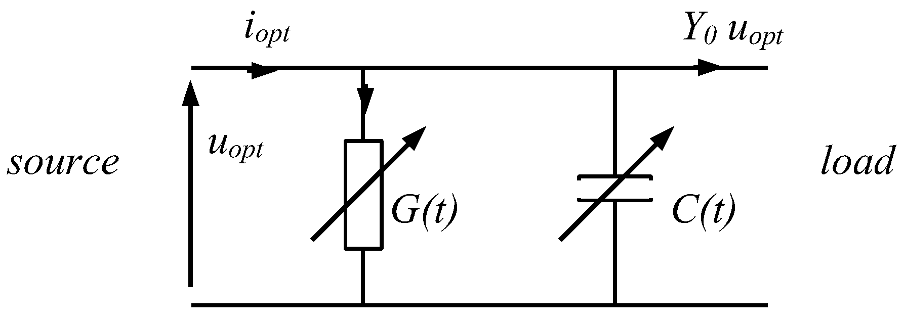
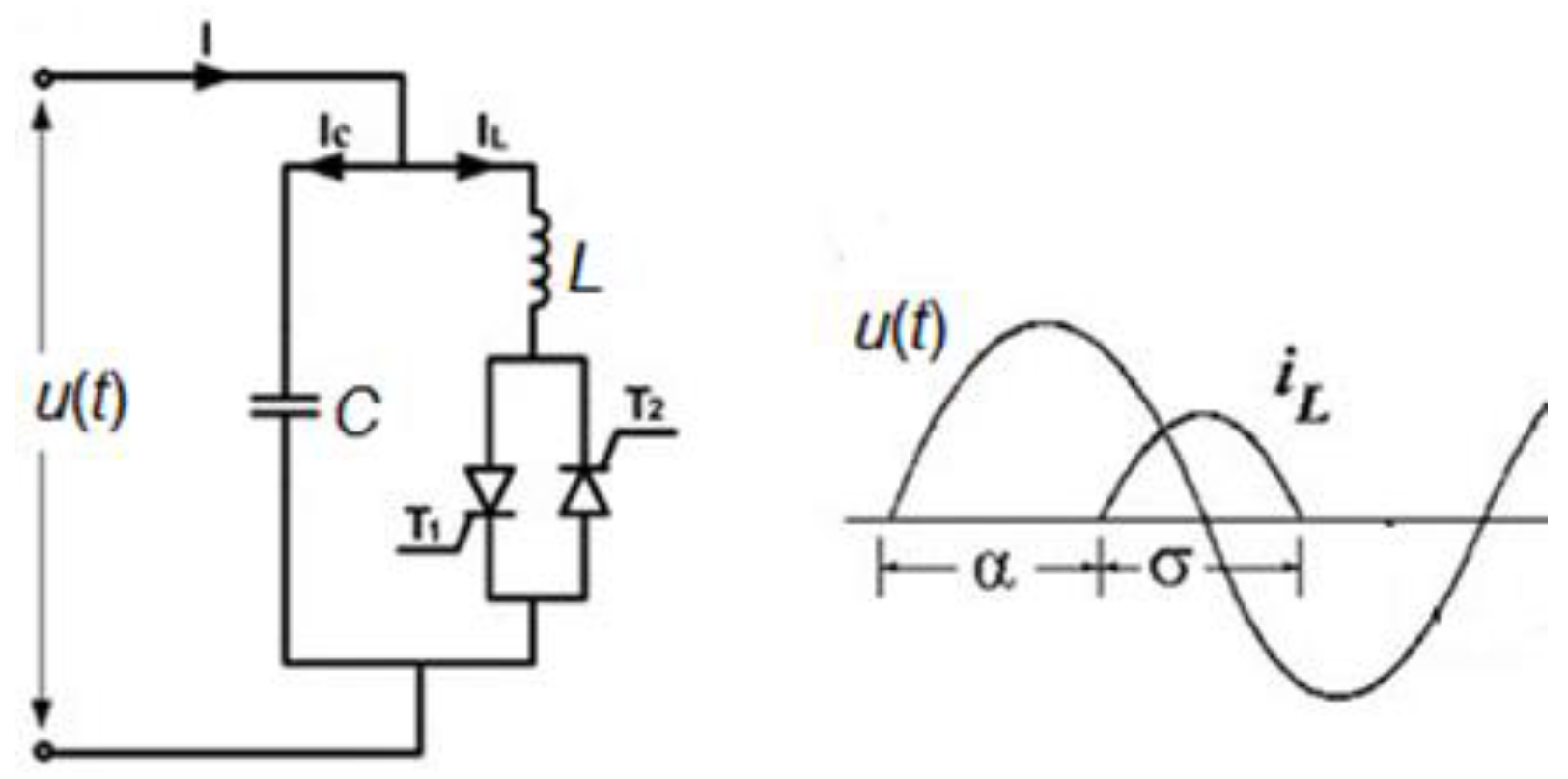
A simple circuit concept with a small number of elements is needed in the practical synthesis of such circuits, for example, a parallel two-terminal compensator. Such a circuit had to be effective for practically every type of load, especially those described by a non-convolution (distorting) operator. Such compensating circuits can be implemented as linear parametric circuits that have high dynamic potential. For example, the parallel connection of the parametric elements G(t), C(t) has proven advantageous. A parallel parametric compensation circuit is shown in Figure 1 below.

This article deals with similar issues, but this time, the parametric impedance is implemented by an active filter in the discrete time domain controlled by a digital filter.

For the first time, the method of control execution of a linear time-variant non-convolution-type two-terminal circuit, over discrete-time and using mathematical feedback (from the formula), is presented. Mathematical feedback implements a specific formula, so this approach is simpler and more versatile than using matched analog/digital regulators.

First of all, in order to calculate the a PWM control signal, it was necessary to present mathematical relations between a periodic current and voltage for such a parametric impedance or admittance operator. Thus, a method of creating a cyclic matrix for parametric impedance, based on the periodization process of the causal parametric operator in discrete time, is presented.

The causal parametric operator of an impedance is formed from the impulse responses of the system due to impulses delivered at every consecutive sample. The impulse responses obtained in this way are arranged in columns below the diagonal.

The detailed procedure of identifying the matrix of a casual parametric operator is presented in the last paragraph.

Creating the cyclo-parametric operator from a casual parametric operator consists of adding samples in one column distant by N samples, where N is the number of samples in one period. Very often, such a cyclo-parametric operator can be obtained from a difference equation using the cyclic unit delay matrix. This matrix should be used on both sides of a difference or recursive equation. In very simple cases, when the impedance with one derivative is implemented, for example, the first derivative of a current signal, the cyclo-parametric matrix is a simple diagonal matrix supplemented with a sub-diagonal matrix and an element of index (1, N).

The whole procedure of creating a cyclo-parametric matrix is presented in this article in detail. On the basis of a cyclo-parametric matrix of a given impedance or admittance operator, it is possible to calculate the duty-cycle for a switched constant voltage source, which allows us, similarly to the previous work, to analyze the performance of the active filter and to analyze the quality parameters of the signals generated by its branch as well as the parameters of the active filter branch itself. In this way, it is possible not only to calculate the current or voltage for a given parametric impedance, but also to calculate the real PWM current waveform generated by the active filter branch. Moreover, the very operators that are used to represent parametric two-terminal circuits can be used to directly calculate steady-state currents and voltages in those circuits and especially to examine the self-excited circuits.

In these cases, such a calculation can answer the question of whether a parametric system will generate spontaneously any current/voltage at a given frequency, i.e., whether the circuit will act as a parametric oscillator. Such an example is also shown in this article.

2. Linear Digital Filters with Variable Parameters

A linear analog digital filter with variable parameters (also: parametric, time dependent, non-stationary) is described by a differential equation

$$\begin{gathered} \begin{array}{c}{a}_0\left(t\right)y\left(t\right)+a_1\left(t\right)\frac{dy(t)}{dt}+a_2\left(t\right)\frac{d^{2}y(t)}{d{t}^2}+\dots +a_M\left(t\right)\frac{d^{M}y(t)}{d{t}^M}\\ \\ =b_0\left(t\right)x\left(t\right)+b_1\left(t\right)\frac{dx(t)}{dt}+b_2\left(t\right)\frac{d^{2}x(t)}{d{t}^2}+\dots +b_N\left(t\right)\frac{d^{N}x(t)}{d{t}^N}\end{array} \end{gathered}$$

(1)

The solution of this equation is determined by the integral operator (resolver)

$$y(t)={\displaystyle \underset{-\infty }{\overset{\infty }{\int }}h(t,t\prime )x(t\prime )dt\prime }.$$

The operator’s kernel $h(t,t\prime )$ usually cannot be found, except by the numerical method when changing it to a digital filter.

When using approximation:

$$y^{(m)}(n\tau )=\frac{1}{{\tau }^m}{\displaystyle \sum _{p=0}^m{(-1)}^p}\frac{m!}{p!(m-p)!}{y}_{n-p}$$

a differential Equation (1)

$${\displaystyle \sum _{n=0}^M{a}_n(t)y^{(n)}(t)}={\displaystyle \sum _{n=0}^N{b}_n(t)x^{(n)}(t)}$$

is replaced by a recursive formula with finite series

$$y_n={\displaystyle \sum _{q\ge 0}^{}{b}_{n,q}^{}{x}_{n-q}}-{\displaystyle \sum _{q\ge 0}^{}{a}_{n,q}^{}{y}_{n-q}}.$$

(2)

The linear operator, resolving this filter, has the following form

$$y_n={\displaystyle \sum _{m=-\infty }^{\infty }{h}_{n,m}{x}_m}$$

(3)

where the sequence $h_{n,m}$ must satisfy the causal-link criterion

$$h_{n,m}=0\hspace{1em}for\hspace{1em}n-m<0$$

and stability condition as well

$$\exists \gamma >0,\forall n\in I\hspace{1em}{\displaystyle \sum _{-\infty }^{\infty }\left|h_{n,m}\right|<\gamma }$$

where I—integer numbers.

The characteristic function of the filter $h_{n,m}$, equivalent to its impulse response, is sought recursively

$$\begin{array}{l}{h}_{n,m}=b_{n,0}^{}{\delta }_{n,m}+b_{n,1}^{}{\delta }_{n-1,m}++b_{n,2}^{}{\delta }_{n-2,m}+\dots \\ -a_{n,1}^{}{h}_{n-1,m}-a_{n,2}^{}{h}_{n-2,m}-\dots \\ ={\displaystyle \sum _{q\ge 0}^{}{b}_{n,q}^{}{\delta }_{n-q,m}}-{\displaystyle \sum _{q\ge 1}^{}{a}_{n,q}^{}{h}_{n-q,m}}\end{array}$$

(4)

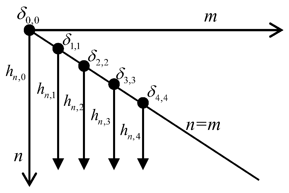
To organize the calculations, the indicator ‘m’ is determined while changing n: n = m, m + 1, … In this way, the matrix $h_{n,m}$ is determined column by column (Figure 2). This procedure can be described as follows (where the symbol ${\delta }_{n,m}$ represent the Kronecker delta):

$$\begin{gathered} h_{m,m}=b_{0,m}^{} \\ {h}_{m+1,m}=b_{1,m+1}^{}-a_{1,m+1}^{}{h}_{m,m} \\ {h}_{m+2,m}=b_{2,m+2}^{}-a_{1,m+2}^{}{h}_{m+1,m}-a_{2,m+2}^{}{h}_{m,m}. \end{gathered}$$

Operator (3) can also be represented in the form of a parametric convolution

$$y_n={\displaystyle \sum _{m=-\infty }^{\infty }{h}_{n,m}{x}_m}={\displaystyle \sum _{m=-\infty }^{\infty }{H}_{n,n-m}{x}_m}={\displaystyle \sum _{m=-\infty }^{\infty }{H}_{n,m}{x}_{n-m}},$$

where

$$H_{n,m}=h_{n,m}\mathrm{or}{H}_{n,m}=h_{n,n-m}.$$

It follows from the causal-link criterion that

$$h_{n,m}=0\hspace{1em}for\hspace{1em}n-m<0$$

thus

$$H_{n,m}=0\hspace{1em}for\hspace{1em}m<0.$$

Therefore, for the causal system, the parametric convolution-operator takes the form

$$y_n={\displaystyle \sum _{m=0}^{\infty }{H}_{n,m}{x}_{n-m}}.$$

(5)

It is therefore a linear non-recursive digital filter with variable weights.

3. Linear Digital Filters with Periodic Parameters

It is assumed that all weights of the filter described by Equation (2) change with the common period of N samples. If the input signal $\left\{x_n\right\}$ also has the same period, then

$$y_n={\displaystyle \sum _{m=-\infty }^{\infty }{h}_{n,m}{\displaystyle \sum _{p=-\infty }^{\infty }{\tilde{x}}_{m+pn}}}={\displaystyle \sum _{p=-\infty }^{\infty }{\displaystyle \sum _{m=-\infty }^{\infty }{h}_{n,m}{\tilde{x}}_{m+pn}}}={\displaystyle \sum _{m=-\infty }^{\infty }{\tilde{x}}_m{\displaystyle \sum _{p=-\infty }^{\infty }{h}_{n,m-pN}}},$$

where $\tilde{x}$ is the N-segment of the x signal, i.e.,

$${\tilde{x}}_n=\{\begin{array}{lll}{x}_n\hfill & for\hfill & n\in \{0,1,\dots ,N-1\}\hfill \\ 0\hfill & \hfill & otherwise\hfill \end{array}.$$

Hence it follows that

$$y_n={\displaystyle \sum _{m=0}^{N-1}{\tilde{h}}_{n,m}{x}_m}$$

for $n\in \{0,1,\dots ,N-1\}$, where

$${\tilde{h}}_{n,m}={\displaystyle \sum _{p=0}^{\infty }{h}_{n,m-pN}}$$

(6)

and

$$\mathit{H}=\left[\begin{array}{cccc}{\tilde{h}}_{0,0}& {\tilde{h}}_{0,1}& \cdots & {\tilde{h}}_{0,N-1}\\ {\tilde{h}}_{1,0}& {\tilde{h}}_{1,1}& \cdots & {\tilde{h}}_{1,N-1}\\ \cdots & \cdots & & \cdots \\ {\tilde{h}}_{N-1,0}& {\tilde{h}}_{N-1,1}& \cdots & {\tilde{h}}_{N-1,N-1}\end{array}\right]$$

is the so-called cycloparametric matrix.

Expression (6) is the so-called generalized-periodization formula, which determines the elements of the cycloparametric matrix using a direct relation between periodic input and output signals of the same period.

It is not difficult to show that the generalized-periodization formula can also be written as follows:

$${\tilde{h}}_{n,m}={\displaystyle \sum _{p=0}^{\infty }{h}_{n+pN,m}}\hspace{1em}n\in \{0,1,\dots ,N-1\}.$$

(7)

Indeed, there is a recursive formula for periodic filter coefficients

$$h_{n+N,m+N}={\displaystyle \sum _{q\ge 0}^{}{b}_{n,q}^{}{\delta }_{n-m-q}}-{\displaystyle \sum _{q\ge 0}^{}{a}_{n,q}^{}{h}_{n+N-q,m+N}},$$

which is the same as for series $\left\{h_{n,m}\right\}$. Therefore

$$h_{n+N,m+N}=h_{n,m}$$

it also follows that

$${\displaystyle \sum _{p=0}^{\infty }{h}_{n,m-pN}}={\displaystyle \sum _{p=0}^{\infty }{h}_{n+pN,m}}.$$

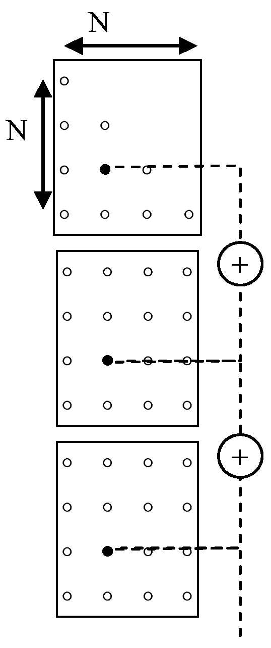
The method to determine matrix elements ${\tilde{h}}_{n,m}$ is illustrated in Figure 3. For this purpose, it is enough to determine N appropriately long columns of the matrix $h_{n,m}$ by recurrence, and then sum up its every N-th element in each column.

The cycloparametric matrix can also be determined directly by inverting the filter’s steady state matrix, provided the system is stable.

The output and input samples of the filter signals are

$$y=\left[\begin{array}{c}{y}_0\\ y_1\\ ⋮\\ y_{N-1}\end{array}\right];x=\left[\begin{array}{c}{x}_0\\ x_1\\ ⋮\\ x_{N-1}\end{array}\right]$$

and the diagonal matrices of filter coefficients are

$$b_i=\left[\begin{array}{cccc}{b}_{i,0}^{}& & & \\ & b_{i,1}^{}& & \\ & & \ddots & \\ & & & b_{i,N-1}^{}\end{array}\right];a_i=\left[\begin{array}{cccc}{a}_{i,0}^{}& & & \\ & a_{i,1}^{}& & \\ & & \ddots & \\ & & & a_{i,N-1}^{}\end{array}\right]$$

and the unit-delay cyclic-matrix is as follows

$$\mathit{P}=\left[\begin{array}{lllll}\hfill & \hfill & \hfill & \hfill & 1\hfill \\ 1\hfill & \hfill & \hfill & \hfill & \hfill \\ \hfill & 1\hfill & \hfill & \hfill & \hfill \\ \hfill & \hfill & \ddots \hfill & \hfill & \hfill \\ \hfill & \hfill & \hfill & 1\hfill & \hfill \end{array}\right];$$

so the filter equation can be written in matrix form

$$(a_0+a_1\mathit{P}+a_2{\mathit{P}}^2+\dots +a_N{\mathit{P}}^N)y=(b_0+b_1\mathit{P}+b_2{\mathit{P}}^2+\dots +b_M{\mathit{P}}^M)x$$

where: M < N, 1—unit matrix, ${\mathit{P}}^i$—i-th power of P matrix, thus

$$y=\tilde{h}x={(a_0+a_1\mathit{P}+a_2{\mathit{P}}^2+\dots +a_N{\mathit{P}}^N)}^{-1}(b_0+b_1\mathit{P}+b_2{\mathit{P}}^2+\dots +b_M{\mathit{P}}^M)x$$

and

$$\mathit{H}={(a_0+a_1\mathit{P}+a_2{\mathit{P}}^2+\dots +a_N{\mathit{P}}^N)}^{-1}(b_0+b_1\mathit{P}+b_2{\mathit{P}}^2+\dots +b_M{\mathit{P}}^M).$$

(8)

As an example, we can consider the steady-state equation of an RL filter with periodically varying coefficients:

$$\begin{gathered} R(t)i\left(t\right)+L(t)\frac{\Delta i(t)}{\tau }=u(t)\to a_0(n\tau )i\left(n\tau \right)+a_{1}i\left((n-1)\tau \right)=u(n\tau ) \\ \left[\begin{array}{lllll}{a}_{0,0}\hfill & \hfill & \hfill & \hfill & a_{1,N-1}\hfill \\ a_{1,0}\hfill & a_{0,1}\hfill & \hfill & \hfill & \hfill \\ \hfill & a_{1,1}\hfill & a_{0,2}\hfill & \hfill & \hfill \\ \hfill & \hfill & \ddots \hfill & \ddots \hfill & \hfill \\ \hfill & \hfill & \hfill & a_{1,N-2}\hfill & a_{0,N-1}\hfill \end{array}\right]\left[\begin{array}{l}{i}_0\hfill \\ i_1\hfill \\ i_2\hfill \\ ⋮\hfill \\ i_{N-1}\hfill \end{array}\right]=\left[\begin{array}{l}{u}_0\hfill \\ u_1\hfill \\ u_2\hfill \\ ⋮\hfill \\ u_{N-1}\hfill \end{array}\right]\to \mathit{H}i=u \end{gathered}$$

where H is the cycloparametric matrix and the vector i can be found by inverting the matrix H.

It is also worth noting that the condition

$$h_{n+N,m+N}=h_{n,m}$$

for a filter operator with periodic variable parameters entails a condition

$$H_{n+N,n-m}=H_{n,n-m}\to H_{n+N,m}=H_{n,m}$$

for the parametric-convolution operator.

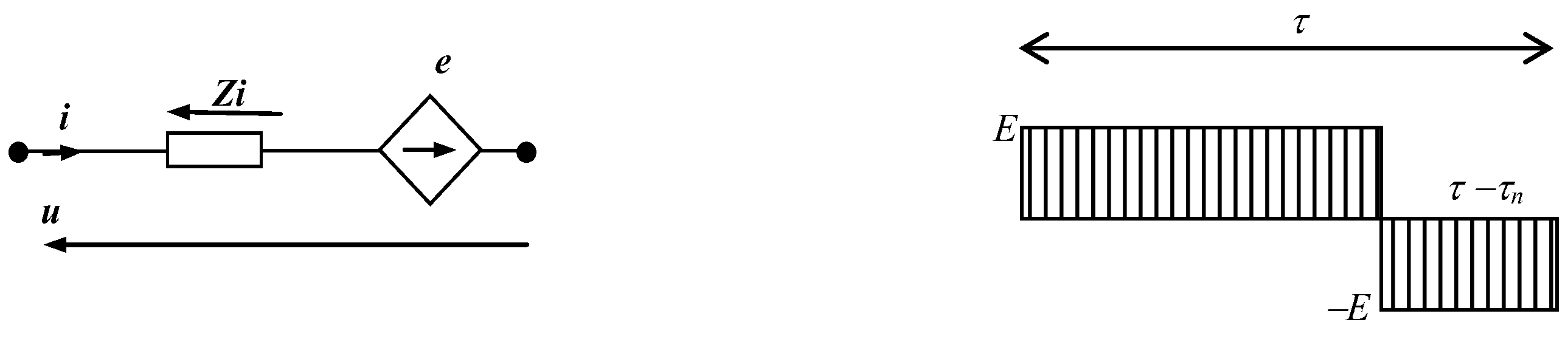
4. Universal Voltage-Controlled Source

A universal voltage source plays a key role in an active-controlled two-terminal network and is realized with the help of an EMF E switched within period τ with duty cycle τ_n/τ.

The branch diagram is shown in Figure 4.

Averaging the square waveform within sampling period τ results in value of the n-th sample of the voltage e(t) [1,16].

$$e_n^{}={\vartheta }_n{E}_{}-(1-{\vartheta }_n)E_{}=(2{\vartheta }_n-1)E_{}$$

${\vartheta }_n$—duty cycle of the voltage source in sample ‘n’, τ—sampling period.

Inverse transformation has the form

$${\vartheta }_n=\frac{1}{2}\left(1+{\overline{e}}_n\right);{\overline{e}}_n=\frac{e_n}{E}$$

(9)

and E (constant voltage) can be taken from the capacity.

5. Implementation of an Immittance Operator

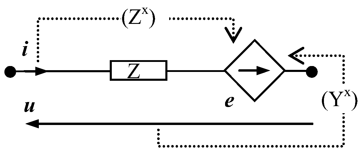
A diagram of a two-terminal network implementing a given linear operator, impedance Z* or admittance Y*, with the use of a voltage-source e(t), controlled by current i(t) or voltage u(t), is shown in Figure 5.

The universal branch in Figure 5 consists of an electromotive force e(t) and a passive component of a given impedance Z.

From the branch equations

$$\begin{gathered} u(t)+e(t)=Zi(t) \\ u(t)=Z^{*}i(t)\mathrm{or}i(t)=Y^{*}u(t) \end{gathered}$$

the formula for controlling e(t) is obtained:

$$e(t)=(Z-Z^{*})i(t)$$

(10)

or

$$e(t)=-(1-Z{Y}^{*})u(t)$$

(11)

6. Implementation of a Given Discrete-Time Immittance Operator

To implement a linear non-periodic time-dependent impedance operator

$$u_n={\displaystyle \sum _{m=0}^{\infty }{Z}_{n,m}^{*}{i}_{n-m}}$$

one needs to control the electromotive force $\left\{{\overline{e}}_n\right\}$ with duty cycles $\left\{{\vartheta }_n\right\}$ according to the following formulas:

$${\overline{e}}_n=\frac{1}{E}{\displaystyle \sum _{m=0}^{\infty }{(Z_m-Z_{n,m}^{*})}_m{i}_{n-m}}$$

$${\vartheta }_n=\{\begin{array}{ccc}\frac{1}{2}\left(1+{\overline{e}}_n\right)& for& \left|{\overline{e}}_n\right|\le 1\\ 0& for& {\overline{e}}_n<-1\\ 1& for& {\overline{e}}_n>1\end{array}$$

(12)

Whereas the implementation of a cycloparametric operator

$$u_n={\displaystyle \sum _{m=0}^{N-1}{\tilde{Z}}_{n,m}^{*}{i}_m}$$

is based on the formula

$${\overline{e}}_n=\frac{1}{E}\left({\displaystyle \sum _{m=0}^n{\tilde{Z}}_{n-m}^{}{i}_m+{\displaystyle \sum _{m=n+1}^{N-1}{\tilde{Z}}_{n-m+N}^{}{i}_m}-{\displaystyle \sum _{m=0}^{N-1}{\tilde{Z}}_{n,m}^{*}{i}_m}}\right)$$

where N is the number of samples per period.

To implement a linear, non-periodic, time-dependent admittance operator in discrete time

$$\begin{gathered} i_n={\displaystyle \sum _{m=-\infty }^{\infty }{Y}_{n,m}^{*}{u}_m}={\displaystyle \sum _{m=-\infty }^{\infty }{\left(Y_{}^{*}\right)}_{n,m}^{|}{u}_{n-m}} \\ {\left(Y_{}^{*}\right)}_{n,m}^{|}=Y_{n,n-m}^{*} \end{gathered}$$

where

$$\begin{gathered} Y_{n,n-m}^{}=0\mathrm{for}n-m<0 \\ {\left(Y_{}^{*}\right)}_{n,m}^{|}=0\mathrm{for}m<0 \end{gathered}$$

One needs to control the electromotive force according to the following formula:

$${\overline{e}}_n=\frac{1}{E}\left(-u_m+{\displaystyle \sum _{m=0}^{\infty }{\left(Z{Y}_{}^{*}\right)}_{n,m}^{|}{u}_{n-m}}\right)$$

with auxiliary operator

$$\begin{gathered} {(Z{Y}^{*})}_{n,m}={\displaystyle \sum _{p=m}^n{Y}_{p,m}^{*}{Z}_{n-p}}\hspace{1em}\mathrm{for}n-m>0 \\ {\left(Z{Y}_{}^{*}\right)}_{n,m}^{|}={\left(Z{Y}_{}^{*}\right)}_{n,n-m}^{} \end{gathered}$$

Its N-periodic implementation is carried out with cycloparametric operators. Thus the admittance operator should have the form

$$\mathrm{s}{i}_n={\displaystyle \sum _{m=0}^{N-1}{\tilde{Y}}_{n,m}^{*}{u}_m}$$

and the EMF $\left\{{\overline{e}}_n\right\}$ is to follow the operator formulas

$$\begin{gathered} {\overline{e}}_n=\frac{1}{E}\left(-u_m+{\displaystyle \sum _{m=0}^{N-1}{\left(Z{Y}_{}^{*}\right)}_{n,m}^{\sim }{u}_m}\right) \\ {\left(Z{Y}_{}^{*}\right)}_{n,m}^{\sim }={\displaystyle \sum _{p=0}^{N-1}{\tilde{Z}}_{n-p\mathrm{mod}\mathrm{N}}}. \end{gathered}$$

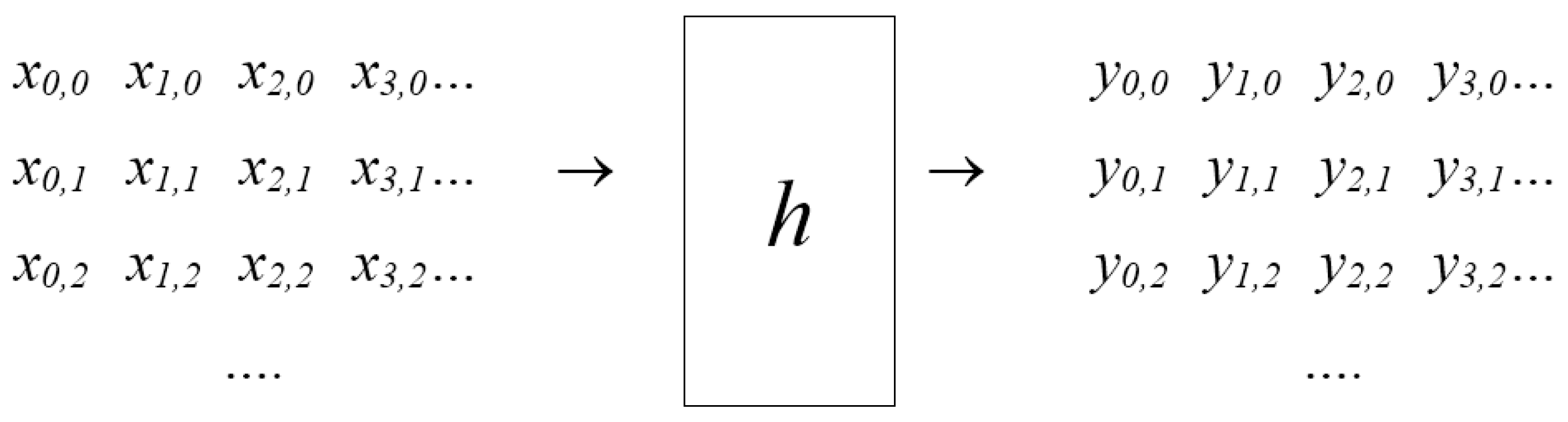
7. Identification of Non-Plane Operators

While the convolution operator can be identified by a single test signal at the input and one at the output of the system (because they are related by a convolution fraction to each other), an infinite set of input signals ${\left\{x_{n,i}^{}\right\}}_{i=0}^{\infty }$ is needed to identify the linear operator h, as illustrated in Figure 6 below.

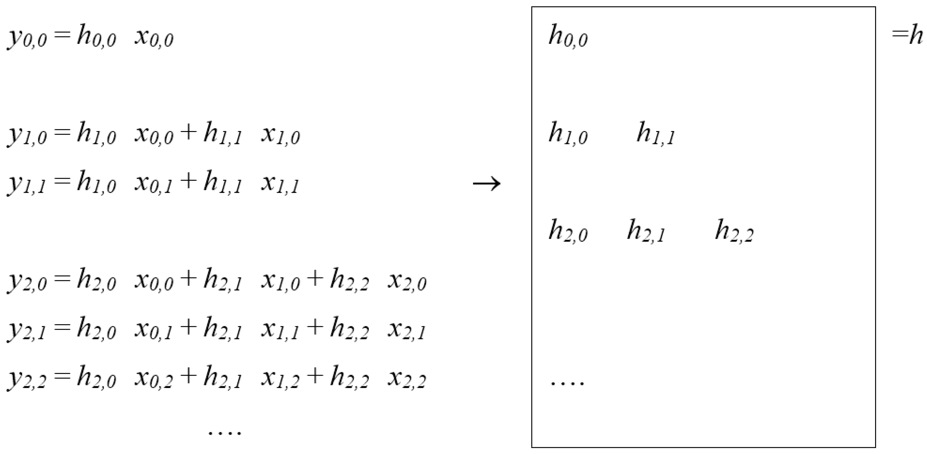
The matrix elements of the operator h lay on diagonal and sub-diagonals, which results from the causality condition, and are determined from the set of linear equations.

From the formula

$$y_{n,i}={\displaystyle \sum _{m=0}^n{h}_{n,m}{x}_{m,i}}$$

the successive systems of linear equations follow (Figure 7):

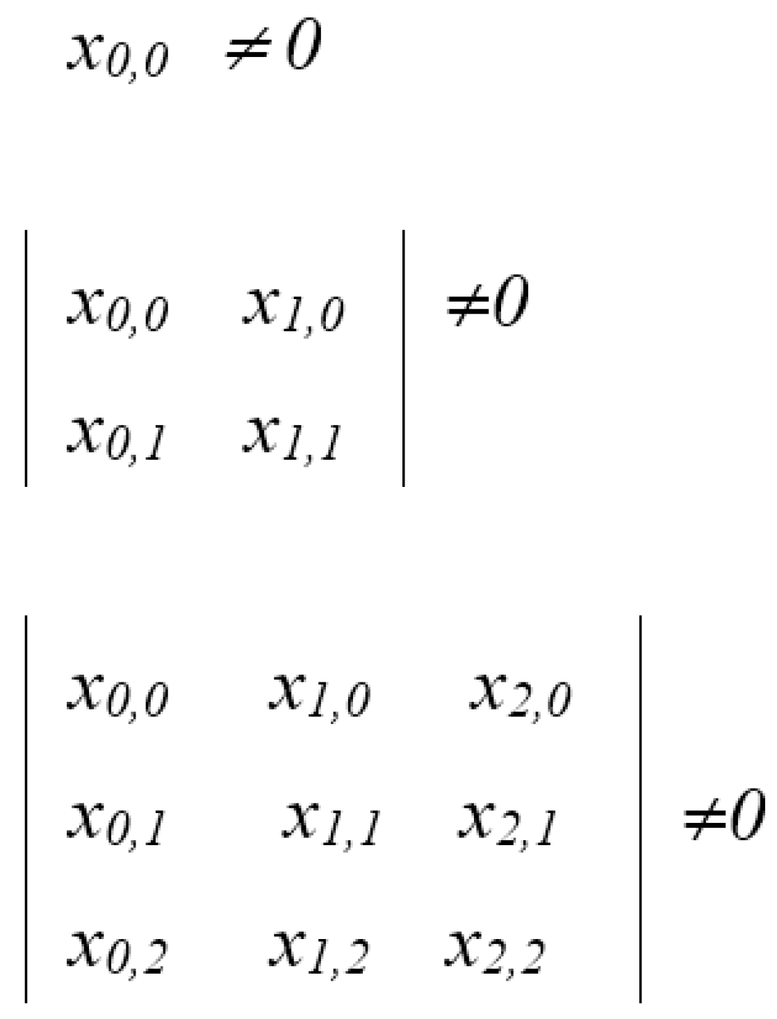
The sizes of the equation systems expand by 1 in each subsequent step. The set of input signals ${\left\{x_{n,i}^{}\right\}}_{i=0}^{\infty }$ must be independent, which takes place when the following determinants are non-zero (Scheme 1).

7.1. Example 1

The governing equation for an RL parametric branch is

$$R(t)i\left(t\right)+L(t)\frac{\Delta i(t)}{\tau }=u(t)\to a_0(n\tau )i\left(n\tau \right)+a_{1}i\left((n-1)\tau \right)=u(n\tau ).$$

From the previous example we have cycloparametric $Z^{*}$ operators

$$Z^{*}=\left[\begin{array}{lllll}{a}_{0,0}\hfill & \hfill & \hfill & \hfill & a_{1,N-1}\hfill \\ a_{1,0}\hfill & a_{0,1}\hfill & \hfill & \hfill & \hfill \\ \hfill & a_{1,1}\hfill & a_{0,2}\hfill & \hfill & \hfill \\ \hfill & \hfill & \ddots \hfill & \ddots \hfill & \hfill \\ \hfill & \hfill & \hfill & a_{1,N-2}\hfill & a_{0,N-1}\hfill \end{array}\right]$$

And, assuming that inner impedance of the universal branch is

$$Z=R+\mathit{sL}\to a\ast i\left(n\tau \right)+b\ast i\left((n-1)\tau \right)=u(n\tau )$$

where

$$a=R+\frac{L}{\tau },b=-\frac{L}{\tau }.$$

we get:

$$e(t)=(Z-Z^{*})i(t)\to \left[\begin{array}{l}{e}_0\hfill \\ e_1\hfill \\ e_2\hfill \\ ⋮\hfill \\ e_{N-1}\hfill \end{array}\right]=\left[\begin{array}{lllll}a-a_{0,0}\hfill & \hfill & \hfill & \hfill & b-a_{1,N-1}\hfill \\ b-a_{1,0}\hfill & a-a_{0,1}\hfill & \hfill & \hfill & \hfill \\ \hfill & b-a_{1,1}\hfill & a-a_{0,2}\hfill & \hfill & \hfill \\ \hfill & \hfill & \ddots \hfill & \ddots \hfill & \hfill \\ \hfill & \hfill & \hfill & b-a_{1,N-2}\hfill & a-a_{0,N-1}\hfill \end{array}\right]\left[\begin{array}{l}{i}_0\hfill \\ i_1\hfill \\ i_2\hfill \\ ⋮\hfill \\ i_{N-1}\hfill \end{array}\right].$$

Hence the needed duty cycles within sampling period τ are

$$\left[\begin{array}{l}{\vartheta }_0\hfill \\ {\vartheta }_1\hfill \\ {\vartheta }_2\hfill \\ ⋮\hfill \\ {\vartheta }_{N-1}\hfill \end{array}\right]=\frac{1}{2}\left(1+\frac{1}{E}\left[\begin{array}{l}{e}_0\hfill \\ e_1\hfill \\ e_2\hfill \\ ⋮\hfill \\ e_{N-1}\hfill \end{array}\right]\right).$$

(13)

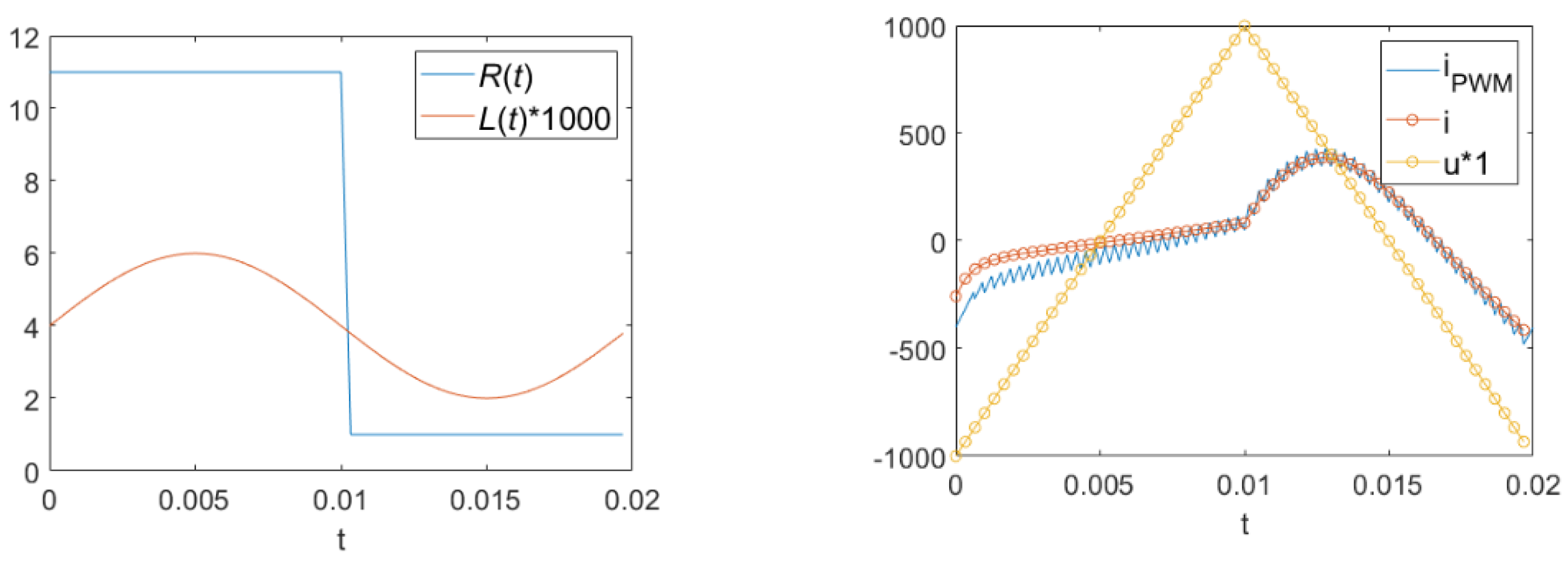
Examples of waveforms of R(t), L(t) and branch voltage u(t) as well as current i(t) for N = 60 are shown below (Figure 8).

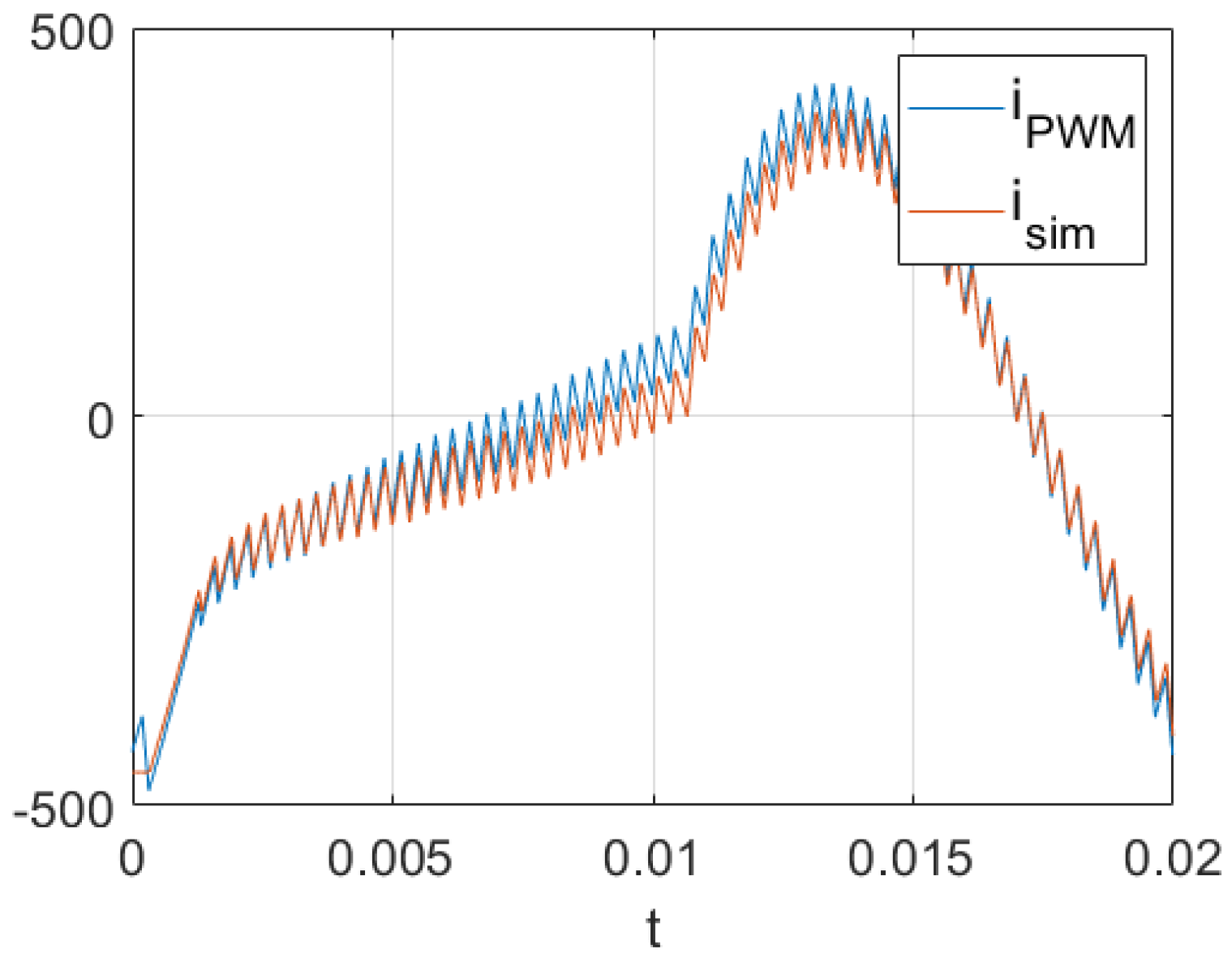
PWM current (i_PWM) can also be calculated using matrix equation (Figure 9)

$$\mathit{u}+{\mathit{e}}_{PWM}=\mathit{Z}{\mathit{i}}_{PWM}$$

where e_PWM is the PWM signal generated according to duty cycles calculated in (13), assuming e_PWM has mean value 0.

To confirm the correctness of the PWM current calculations, a simulation was carried out in Matlab/Simulink using the real Full-Bridge Converter model.

This model has two non-zero parameters, Device on-state resistance and Snubber resistance, which slightly influenced the current waveform from the simulation in relation to the current calculated on the basis of the formula—see Figure 9.

7.2. Example 2

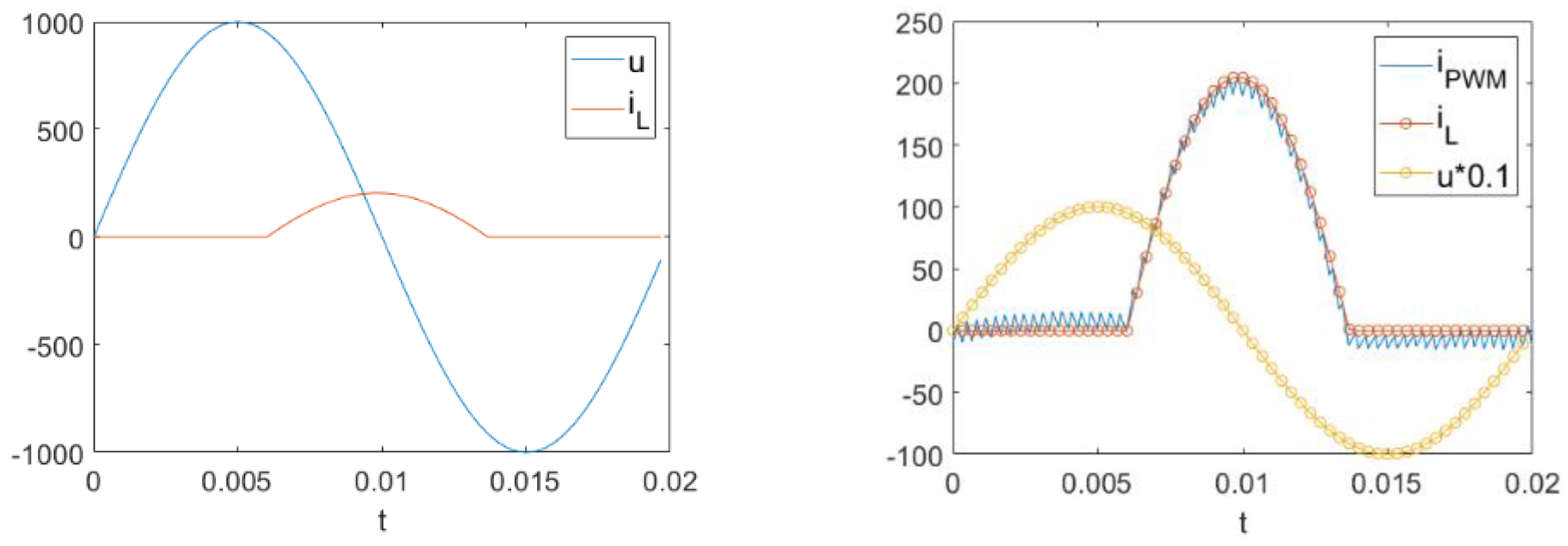
Let us consider a Static Var Compensators (SVC) branch with parametric (switched on/off) inductance (Figure 10).

And a static capacitor $C\frac{du(t)}{dt}=i_C(t)$. Its cycloparametric matrix is

$$Y_C{}^{*}=\frac{C}{\tau }\left[\begin{array}{lllll}1\hfill & \hfill & \hfill & \hfill & -1\hfill \\ -1\hfill & 1\hfill & \hfill & \hfill & \hfill \\ \hfill & -1\hfill & 1\hfill & \hfill & \hfill \\ \hfill & \hfill & \ddots \hfill & \ddots \hfill & \hfill \\ \hfill & \hfill & \hfill & -1\hfill & 1\hfill \end{array}\right]$$

For parametric inductance, the cycloparametric matrix $Y_L{}^{*}$ is

Thus, the cycloparametric matrix $Y^{*}$ for SVC branch is

$$Y^{*}=Y_C{}^{*}+Y_L{}^{*}$$

and

$$se(t)=-(1-Z{Y}^{*})u(t)$$

where Z is the inner impedance of the universal branch.

Hence, the needed duty cycles of the voltage source in discrete time are to be calculated from

$${\vartheta }_n=\frac{1}{2}\left(1+{\overline{e}}_n\right);{\overline{e}}_n=\frac{e_n}{E}$$

Resulting signals are depicted in Figure 11.

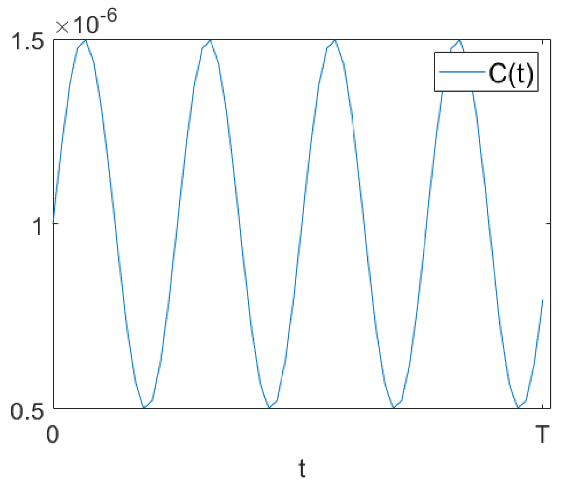
7.3. Example 3

Let us consider a parametric RLC oscillator [17,18] exited by a DC voltage. Its governing equation is

$$1=Ri\left(t\right)+L\frac{di\left(t\right)}{dt}+{\displaystyle \int \frac{i\left(t\right)}{C\left(t\right)}dt}$$

which transforms to the matrix equation

$$1=\left(R*\mathit{E}+L*\mathit{D}1+\mathit{Z}\mathit{c}\right)\mathit{i}$$

where

$$\begin{gathered} \mathit{D}1=\frac{1}{\tau }\left[\begin{array}{lllll}1\hfill & \hfill & \hfill & \hfill & -1\hfill \\ -1\hfill & 1\hfill & \hfill & \hfill & \hfill \\ \hfill & -1\hfill & 1\hfill & \hfill & \hfill \\ \hfill & \hfill & \ddots \hfill & \ddots \hfill & \hfill \\ \hfill & \hfill & \hfill & -1\hfill & 1\hfill \end{array}\right];\mathit{E}=\left[\begin{array}{lllll}1\hfill & \hfill & \hfill & \hfill & \hfill \\ \hfill & 1\hfill & \hfill & \hfill & \hfill \\ \hfill & \hfill & 1\hfill & \hfill & \hfill \\ \hfill & \hfill & \hfill & \ddots \hfill & \hfill \\ \hfill & \hfill & \hfill & \hfill & 1\hfill \end{array}\right] \\ \mathit{Zc}={\left(\mathrm{diag}(\mathit{C})\ast \mathit{D}1+\mathrm{diag}(\mathit{D}1\ast \mathit{C})\right)}^{-1};\mathit{C}=\left[\begin{array}{c}c\left(0\right)\\ c\left(\tau \right)\\ \\ c\left(\tau (N-1)\right)\end{array}\right] \end{gathered}$$

Parametric capacitance in farads is shown in Figure 12.

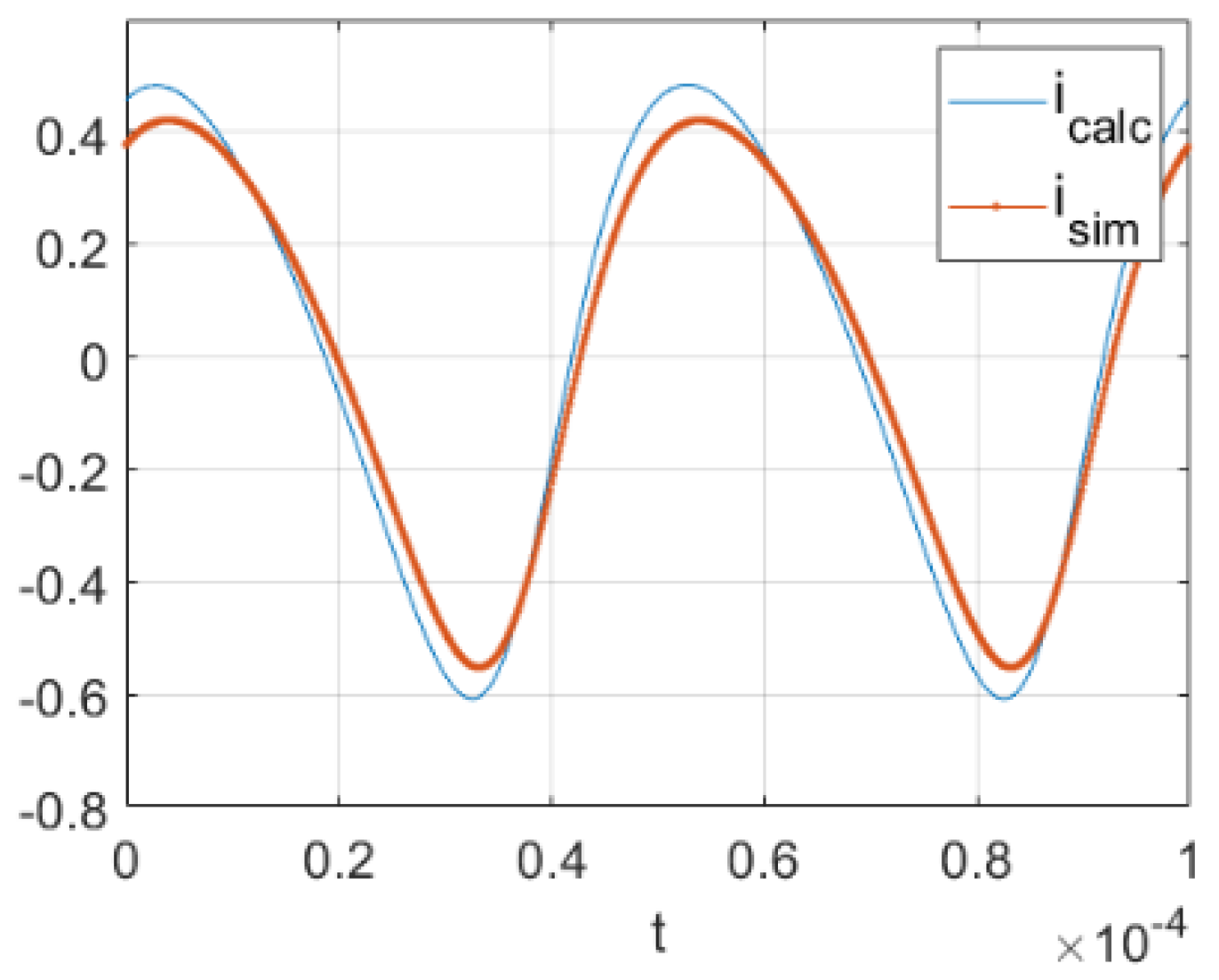
The calculated current as well as one resulting from simulation in Matlab is shown in Figure 13.

The differences between signals are small, bearing in mind that both come from numerical approximations.

In the above examples, apart from the results of matrix calculations, the results of computer simulations carried out in the Matlab environment are also presented. The performed comparisons show that the matrix calculation method is as effective as real-time simulation. The first advantage of the calculation method is that, unlike the simulation where the time to reach steady state is sometimes very long, in the matrix calculation method the target steady signal is calculated in one mathematical operation, i.e., by inverting the matrix-operator of the active-branch. Moreover, given that the periodically changing parameters repeat over a longer cycle, it is not necessary to compute the inverse operator matrix through a longer time in a steady-state operation of the apparatus. The very method of calculating, based on the use of impedance operator, also enables a quick analysis of the system for design purposes and qualitative assessment of the generated current/voltage signals.

8. Conclusions

This article deals with an actively-controlled two-terminal network implementing a non-convolution-type (non-stationary) immittance operator.

The immittance operator is a non-recursive digital filter with variable parameters and is represented as a cycloparametric matrix.

The method of creating a cyclic matrix for parametric impedance based on the periodization process of the causal parametric operator in the discrete time domain was presented.

The causal parametric operator of an impedance was created from the impulse-responses of the system to impulses delivered with sampling period intervals. The impulse responses obtained in this way are arranged in columns below the diagonal.

The detailed procedure on how to identify a parametric operator matrix is presented in the last paragraph. For each row of the operator matrix, solving the same number of linear equations as the number of elements placed in this row is required. Additionally, the conditions for the linear independence of these equations are given. The test signal can be not only a set of pulses but it can be any waveform. However, the samples of the test signal must meet the conditions of non-zero determinants.

When creating the so called cyclo-parametric operators, generally we need to sum the elements in one column distant by N samples, where N is the number of samples in a period, although very often such a cyclo-parametric operator can be obtained from a difference equation using the cyclic unit-delay matrix.

Such matrix formulae allow for direct calculation of periodic signals in a steady-state, and are also fast and easy to use for optimization tasks like system parameters optimization because they do not require separate signal simulations that always have a transient state and lead to a significantly longer computation time.

The entire procedure for creating cyclo-parametric matrices and electric two-terminal equations is detailed in this article.

On the basis of a cyclo-parametric matrix of a given impedance or admittance, it is possible to calculate the duty cycle for a switched constant voltage source, which allows us, similarly to the previous work [19], to analyze the operation of the active filter system and analysis of the parameters of the active filter branch itself. In this way, it is possible not only to calculate the current or voltage for a given parametric impedance but also to calculate the true PWM current waveform generated by the active filter-branch.

For other parametric circuits, such a calculation may also answer the question of whether the system will spontaneously generate some current/voltage frequencies, i.e., whether it will act as a parametric oscillator. Such an example was also shown in this article.

For an active filter-branch the simple formula for the duty-cycle of a switched voltage source was derived: ${\vartheta }_n=\frac{1}{2}\left(1+{\overline{e}}_n\right)$. The formula allows us to make a direct calculation of the duty-cycle in an analytical manner without the use of any auxiliary signals, e.g., sawtooth signals, or any control systems, e.g., a PI controller.

Determining the duty cycle allows us not only to correctly choose the switching frequency and voltage value for the switched voltage source but also allows us to trace the parameters of the current signal that will be generated in the real active filter system.