An Advanced TRACE Modeling Approach: Automatic Connection of 3D Cartesian and Cylindrical VESSEL Components in Integral Plant Models

Abstract

Best estimate system thermal-hydraulic codes in the nuclear engineering community, e.g., TRACE, RELAP3D, CATHARE-3, etc., were extended with 3D coarse-mesh components to better describe the 3D Thermal-Hydraulic (TH) phenomena taking place within the Reactor Pressure Vessel (RPV) and the core. The RPV is usually shaped like a cylinder while the core is mostly a cube. Hence, the TRACE code is equipped with a Cylindrical VESSEL and a Cartesian VESSEL. The former one is to represent the RPV (including core), pressurizer, and steam generator. The latter one is more appropriate to represent the core. The two components are connected by two Vessel-Junctions (VJ) at the core inlet and outlet. Due to the different nodalization between the two VESSELs, the analyst needs to do repetitive and error-prone work defining the cell-to-cell junctions and their TH parameters. To facilitate this process, the Karlsruhe Institute of Technology (KIT) has developed an automatic approach based on a mesh-constructing and field-mapping library, namely the MEDCoupling. These new capabilities of TRACE are demonstrated by the analysis of the coolant mixing for an academic case and the AP1000 reactor.

1. Introduction

The use of 3D Thermal-Hydraulic (TH) codes including system codes with 3D coarse mesh (like TRACE [1] and RELAP5-3D [2]), 3D porous-media, quasi-3D subchannel, and CFD codes for transient analysis of Nuclear Power Plants (NPP) is a tendency nowadays in the nuclear community. Among them, TRACE (TRAC/RELAP Advanced Computational Engine) is a best-estimate reactor system analysis code developed by the U.S. NRC for the analysis of design basis accidents of light water reactors. The use of the coarse-mesh 3D VESSEL components in TRACE is intended to be used to better describe the TH phenomena in the primary circuit and the core of Light Water Reactors (LWR) or Small Modular Reactors (SMR) during non-symmetrical transients, e.g., Main Steam Line Breaking (MSLB) accident, boron dilution, etc., where 3D TH processes are important.

Usually, the flow behavior in the downcomer, the lower plenum, the reactor core, and the upper plenum is treated as 3D flow using the Cylindrical VESSEL with coarse mesh in TRACE. In recent years, a Cartesian 3D VESSEL was added to TRACE for better modeling of the core. The two 3D VESSELs connect through plenty of PIPE components (as Junctions). There, the PIPE positions (based on the spatial correspondence between the flow channels of the two different VESSELs), as well as their thermal-hydraulic definitions, need to be determined by the analyst. That information could be given either in the standard ASCII input file or by defining the Vessel-Junction (VJ) components in the pre- and post-processor SNAP [3]. The well-known French system TH code CATHARE has also applied a similar approach which uses 3D Cylinder and Cartesian Vessels to model the RPV and core, from version 3 [4].

The connections of the two 3D Vessels usually require the specifications of the positional correspondence for dozens and hundreds of flow junctions including their flow areas and the hydraulic diameters at the core inlet and outlet. CATHAE-3 uses its GUI-tool GUITHARE [5] to handle this process [6,7]. In TRACE, this approach usually requires the analyst to define those parameters manually. These operations are repetitive and error prone. In addition, another drawback of this method is the poor accuracy since the calculation of TH parameters often involves irregular intersections of two channels, which hardly can be managed manually.

Consequently, KIT started the development of an innovative multi-vessel coupling approach that automatizes all operations involved in the vessel-coupling process, where the VJ component is no longer needed. For it, we selected the mesh-constructing and field-mapping MEDcoupling library [8] to take advantage of its automatic interpolation functionalities of meshes and fields. This library plays a key role in specifying the spatial correspondence of flow channels and calculating the necessary TH parameters. For this purpose, the low-level data structure of TRACE was significantly restructured. This variant of TRACE is an internal code of KIT at present. Nevertheless, its functional implementation to the official release is possible.

In this paper, the Cylindrical VESSEL is hereinafter referred to as the CY-V while the Cartesian VESSEL is referred to as CA-V.

Finally, it is worth mentioning that the multi-scale coupling approach for different thermal-hydraulic codes is also being developed where system TH codes are being coupled with the subchannel and with CFD codes for an improved description of 3D phenomena inside the primary circuit and the core of NPPs. A recent overview paper summarized these activities [9].

This paper briefly introduces the TRACE code emphasizing the functionalities of the 3D VESSEL components in Section 2. Then, the MEDcoupling library and the automatic coupling approach based on it are described in Section 3. In Section 4, the new capability of TRACE for multi-VESSEL coupling is demonstrated by the analysis of two coolant mixing problems in the RPV of two different reactors, i.e., a generic four-loop PWR and the AP-1000 reactor. Finally, the conclusions and outlook are presented.

2. The TRACE Code

2.1. Basics of TRACE

TRACE is the best-estimate system thermal-hydraulic code of the U.S. Nuclear Regulatory Commission (NRC) for the analysis of design basis accidents of LWR. It solves a system of six conservation equations in the two-fluid formulation for 1D and/or 3D single and/or two-phase flow. There are two options available for the solution: the semi-implicit method and the Stability-Enhancing Two-Step (SETS) method. Together with some essential closure correlations, TRACE can describe the key phenomena inside pipes, valves, reactor pressure vessels, pumps, steam generators, etc. Those structures in TRACE are represented as some type of component, e.g., PIPE, VALVE, VESSEL, and PUMP. Among them, VESSEL is the special 3D component with the capability to describe spatial thermal-hydraulics. It is used mainly to represent the RPV. Nevertheless, it can also represent a steam generator or a pressurizer. TRACE has two types of VESSEL. They are the 3D (r, θ, z) Cylindrical VESSEL–CY-V (Figure 1a), and the 3D (x, y, z) Cartesian VESSEL–CA-V (Figure 1b). The former normally simulates the whole RPV while the latter often models the core particularly. The joint use of CY-V and CA-V can improve the prediction accuracy in the core area during a system-scale simulation. Properly managing the coupling between the VESSELs needs significant effort. Therefore, a separate section contributes the related illustration.

2.2. Current Coupling between the Cylindrical and Cartesian VESSELs

In this section, we use the RPV of AP1000 to demonstrate the coupling rules between CY-V and CA-V. Figure 2 exhibits the basic configurations of the AP1000 primary circuit, which includes the RPV, the hot/cold legs, and the pumps. The coolant enters the RPV through the four cold-legs. It heats up in the reactor and flows out of the RPV to the two hot-legs. There are two primary loops. Each of them corresponds to one hot-leg and two cold-legs.

The TRACE model of the RPV includes a CY-V (for the RPV), a CA-V (for the core), and several additional components as the RPV inlets/outlets. Furthermore, as it was pointed out in the introduction, the two VESSEL components connect each other through the Vessel Junction (VJ) components. Figure 3 displays the overall configuration of the TRACE model, where the core is represented by the Cartesian VESSEL and the RPV by the Cylindrical one.

As depicted in the figure, the RPV has four inlets and two outlets. Every two inlets and one outlet correspond to one primary loop (AP1000 has two primary loops). The two VJs connect the VESSELs at the core inlet and outlet, respectively. Their definition panel in SNAP is shown in Figure 4. In the upper part of the panel, users can view the axial cross-sections of the two VESSELs. The lower part is the parameterized definition window. Here, users must specify the spatial correspondence of the channels and the TH parameters (flow areas and hydraulic diameters) for each junction. Each VJ could consist of dozens or hundreds of such junctions.

The determination or calculation of such parameters sometimes may be very difficult. Take the AP1000 model as an example, the axial cross-sections of the CY-V and CA-V are depicted in Figure 5a,c. By overlapping the two planes, the complicated cell intersections become apparent, Figure 5b. It calls for careful attention to determine the contributions from one cylindrical cell to one Cartesian cell, and vice versa. This is a significant workload for the users. This is also the reason why the manual calculation of the hydraulic parameters may be error prone.

3. The Automatic Coupling Approach between the Cylindrical and Cartesian VESSELs

3.1. The MEDCoupling Library

The MEDCoupling is a built-in library of the SALOME platform. It is released following the SALOME distribution rules. Nevertheless, it is also available as an independent package. The MEDCoupling library is a kind of toolkit that gathers several powerful functionalities around the input and output data of simulation codes (meshes and fields mainly). It is an advanced Application Programming Interface (API) to deal with meshes and fields in memory. The meshes and fields especially refer to the MED format. MED is a broad concept that involves many derivational concepts, e.g., a data format, a library, an API, etc. MEDCoupling is a sort of a logical subset of MED.

With some other sub-libraries, MEDCoupling can construct/modify, write/read meshes and fields in MED format. Furthermore, it can interpolate or map two different meshes to translate the fields between the meshes. This is the key feature that makes the automated multi-vessel coupling possible in our case. The MEDCoupling library was already implemented into TRACE to construct the 3D and 2D meshes of the CY-V (Figure 6, left) [10]. This functionality is the base of the multi-scale coupled codes TRACE/SCF [11] and TRACE/TrioCFD [12] where mesh/fields translation plays a key role. This paper constructs the 3D and 2D meshes of the CA-V component (Figure 6, right, the AP1000 model). Based on these meshes, the new multi-vessel coupling technique is illustrated in the following subchapters.

3.2. Mechanism of the Approach

The new multi-vessel coupling method is developed to release users from the heavy workload of manually defining the VJ components. With this new method, the AP1000 case demonstrated in Figure 3 now is simplified to Figure 7, where the VJ components are no longer necessary. This is a fully automated method based on both high-level and low-level mechanisms, which will be explained hereafter.

3.2.1. High-Level

The new version of TRACE at KIT now can be compiled in two modes: with or without the advanced functionalities for VESSEL coupling. It was initially checked that the modified TRACE version predicts the same results as the original one and no functionalities of the original version deteriorate, with a couple of simple test cases.

In the case of the extended TRACE version, the VESSEL components in the plant model that represent the RPV are identified first, i.e., the VESSEL components that model other structures, e.g., pressurizer, are ignored. If there is no VESSEL for RPV, the code runs in the same manner as the original TRACE version. If there is only one CY-V representing the RPV, the VESSEL-coupling logic is skipped and the functionalities for the post-processing of the VESSEL are available. If a CY-V (for RPV) and a CA-V (for core) exist, the VESSEL-coupling logic is activated. The key steps of this approach are illustrated in Figure 8 (AP1000 TRACE model).

Each step is characterized as follows:

(1)

Identification of the VESSEL components representing an RPV, a core, and, e.g., a pressurizer. The latter VESSEL will be ignored;

(2)

Generation of 2D meshes by the MEDcoupling library for the components CY-V and CA-V using the geometrical data;

(3)

Identification of the core inlets and outlets. The flow area data at those interfaces would be extracted from TRACE memory and written to the 2D meshes;

(4)

Interpolation between the cylindrical and Cartesian 2D meshes. Construction of the inter-junctions between the two VESSELs. The TH parameters of each junction are computed and stored in the fields of the 2D meshes.

It is worth noting that at present only one CY-V (for RPV) and one CA-V (for core) are coupled automatically by this approach.

3.2.2. Low-Level

By defining the VJ component in SNAP, users can establish the relationship between the two VESSELs. This is the traditional way to handle the VESSEL coupling problem with the original TRACE version. In this case, once the VJ component is defined, two bundles of PIPE components are inserted into the TRACE input deck. They act as the junctions at the core inlet and outlet between the two VESSELs. Those complementary PIPEs are processed by the TRACE input routines as normal components, Figure 9.

The final goal of the automatic VESSEL-coupling approach is to construct the two bundles of PIPEs as well. However, they are constructed by the MEDCoupling library automatically, and hence, no manual definition by the user, e.g., in SNAP is needed. Another significant difference is the fact that the complementary PIPEs are not present in the input deck. They are not normal components so they are not processed by TRACE’s regular input routines. Instead, they are automatically generated after the input processing because their construction depends on the geometries of the VESSELs. Furthermore, their information is directly inserted into the memory and the TRACE data structure in the runtime dynamically. Thus, a major modification of the TRACE source was necessary to handle it.

4. Testing the Automatic VESSEL-Coupling Approach

The automatic VESSEL-coupling technique was tested with two coolant mixing cases. One is performed in a generic four-loop PWR and the other in the AP1000 reactor.

4.1. The Coolant Mixing in a Four-Loop PWR

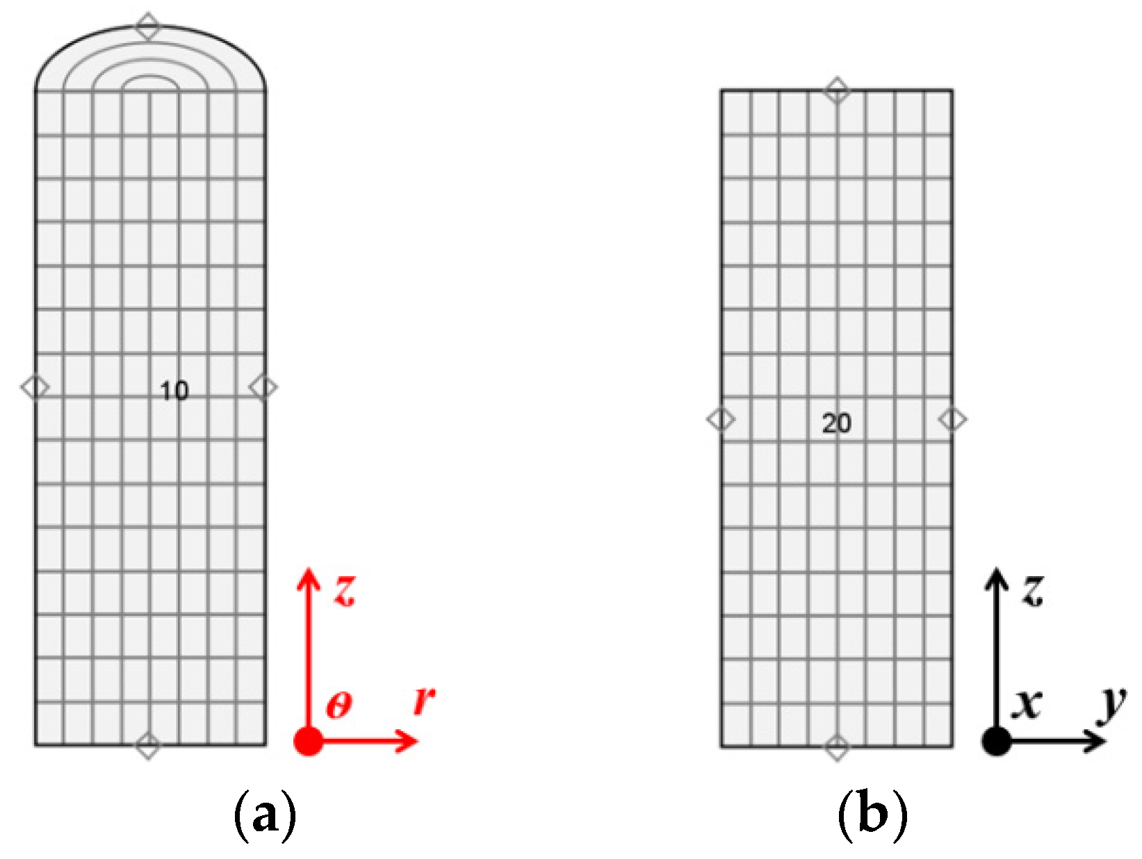
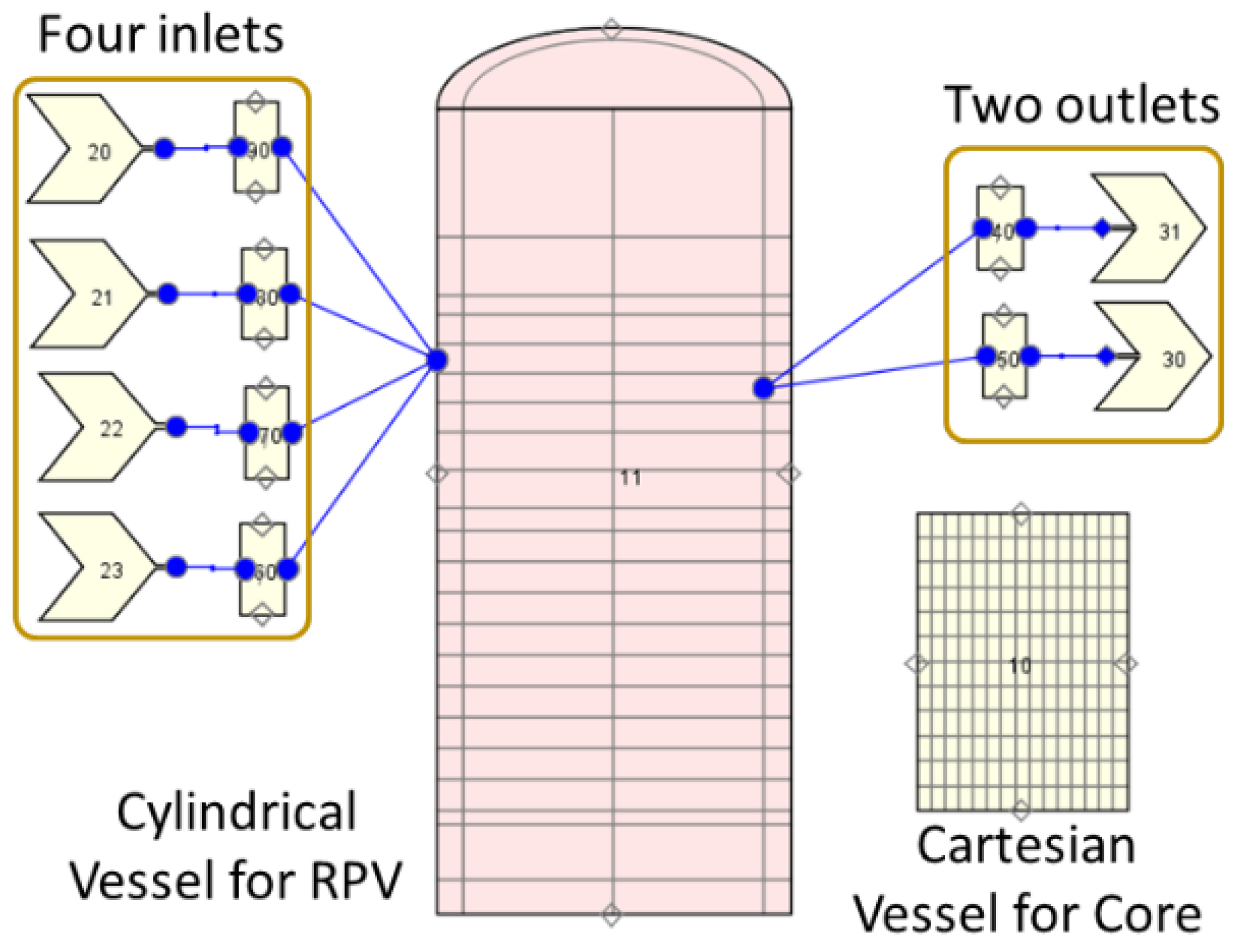
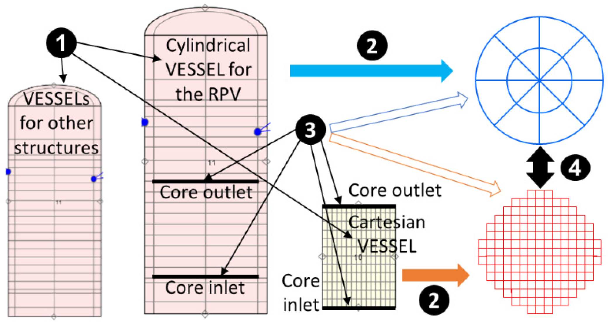
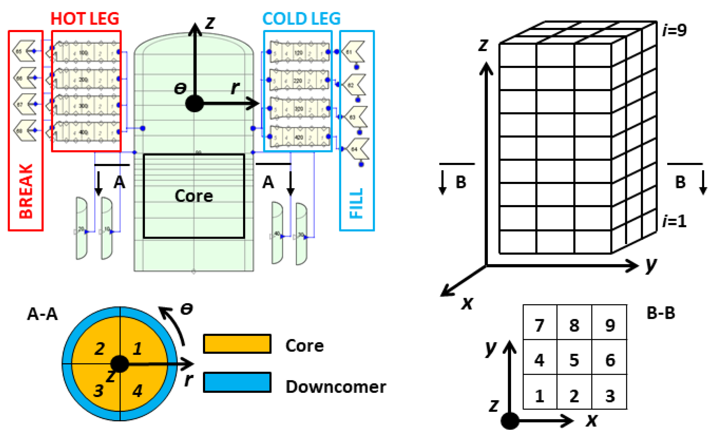
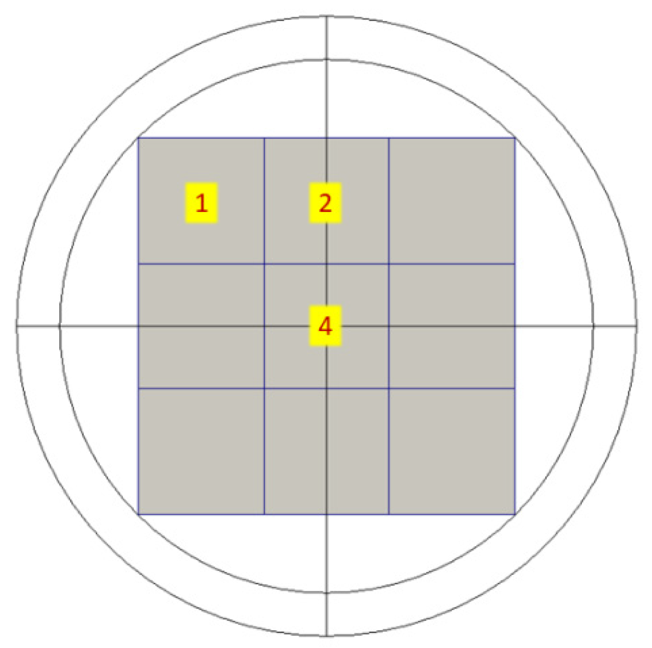
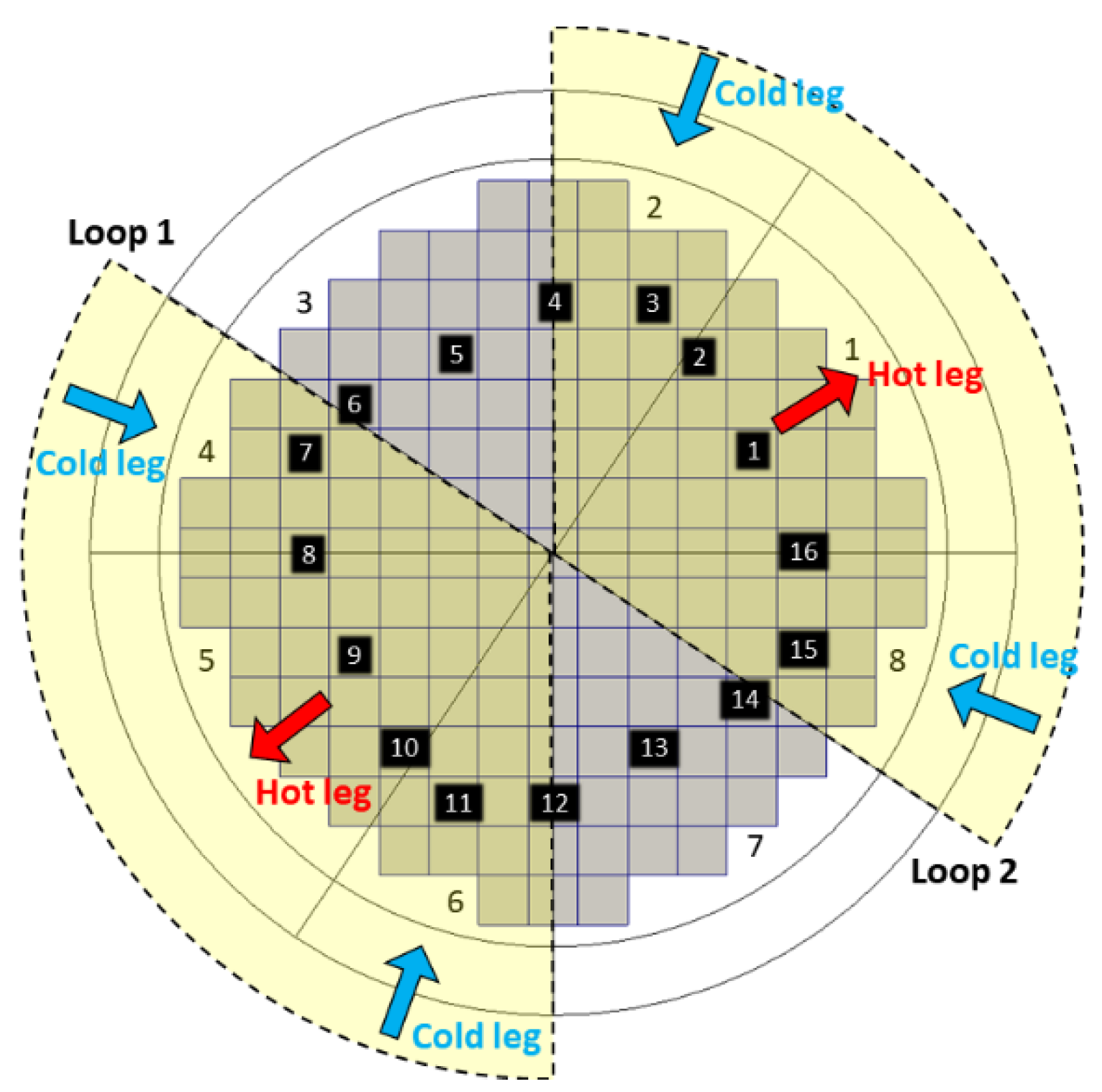
The TRACE model consists of an RPV represented by a CY-V, a core represented by a CA-V, hot-legs, and cold-legs. The overall RPV height and radius are 12.245 and 1.7002 m. It is discretized into 16 axial nodes, 4 azimuthal nodes, and 2 radial nodes. The reactor has four hot-legs and four cold-legs symmetrically connected to the RPV. In this model, the circuits are not considered. The Cartesian Vessel is subdivided into nine square fuel assemblies arranged in a 3 × 3 matrix. Figure 10 shows the TRACE models for the RPV and the core.

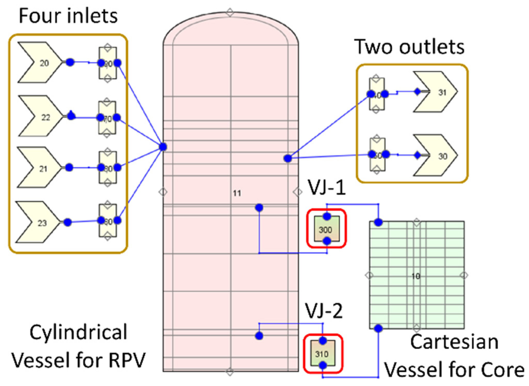
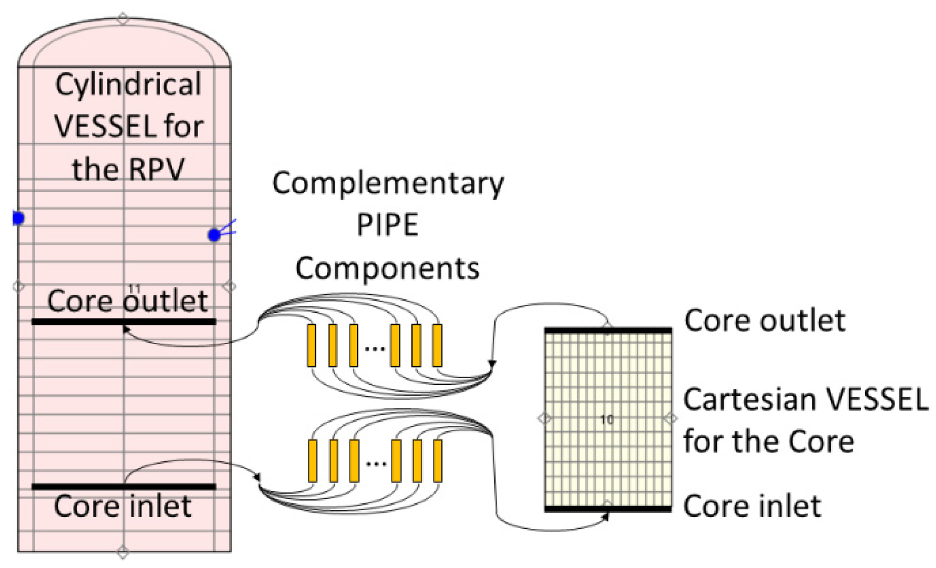
Four FILL and BREAK components are connected to a portion of the cold and hot legs to define the boundary conditions of the problem, e.g., loops mass flow rate, coolant temperature, and pressure. The coolant enters the cold legs, then flows into the downcomer of the RPV and from there to the lower plenum where the flow changes direction and flows upwards entering into the core bottom. The coolant flows through the core and enters the upper plenum. Finally, it exits the RPV and flows into the BREAKs through the hot legs. The core is modeled by the Cartesian VESSEL, which is connected to the RPV-axial face Nr. 2 (core inlet) and the axial face Nr. 11 (core outlet). Hence, the core region in the CY-V is blocked, i.e., no coolant flows through it. Please take Figure 9 as a reference. Once the code is launched, the steps listed under Section 3.2.1 are performed sequentially. According to the VESSEL components configuration, 32 additional PIPEs (as Junctions connecting the two VESSEL components) are constructed and inserted into the TRACE data structure automatically. In total, 16 of them are at the core inlet plane and 16 are at the core outlet plane. 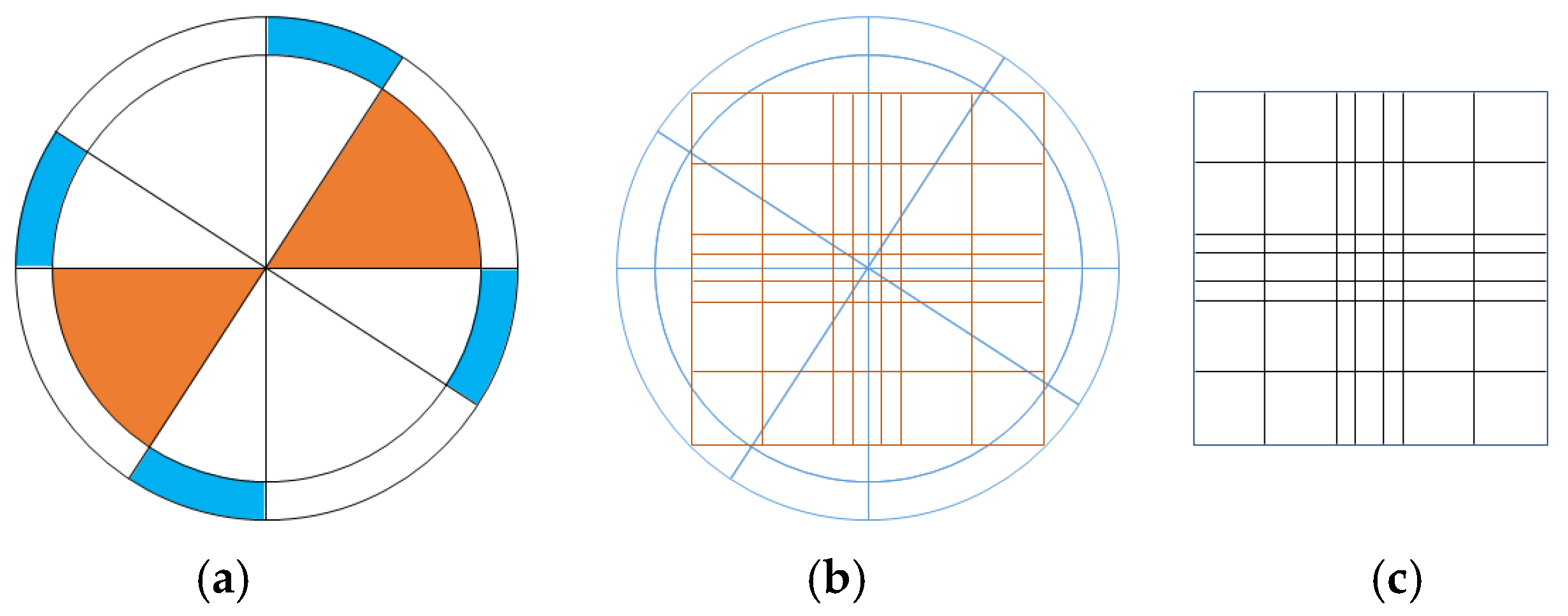Figure 11 illustrates the quantitative distribution of the additional PIPEs from the point of the CA-V (1 × 4 + 2 × 4 + 4 × 1 = 16).

TRACE first runs a Steady-State (SS) simulation. During the SS, the inlet velocity at loop1 is 15 m/s. Inlet velocities of the other three loops are identical to 10 m/s. The inlet coolant temperature is 400 K. The outlet pressure is 15.55 MPa. After the SS, a TRACE transient (TS) simulation is carried out. The total problem time is 50.0 s. The boundary conditions for the transient are given in

Table 1. The boundary conditions during the transient.

	Inlet Velocity [m/s]	Inlet Temperature [K]		Outlet Pressure [MPa]
Time	0~50 s	0~35 s	35~50 s	0~50 s
Loop 1	15	400–500	500	15.55
Loop 2~4	10	400		15.55

.

The cold coolant and hot coolant first mix a little bit in the CY-V downcomer. Then, the main mixing effect happens in the CY-V lower plenum. The coolant then flows from the CY-V lower plenum to the CA-V core and there in the core some mixing would happen. Next, the coolant flows out of the CA-V core and to the CY-V upper plenum. There the final mixing takes place. Particularly for this testing case, what we are concerned about is whether the coolant can flow between the two VESSELs properly and whether the coolant mixing effect behaves rationally in/between the two VESSELs.

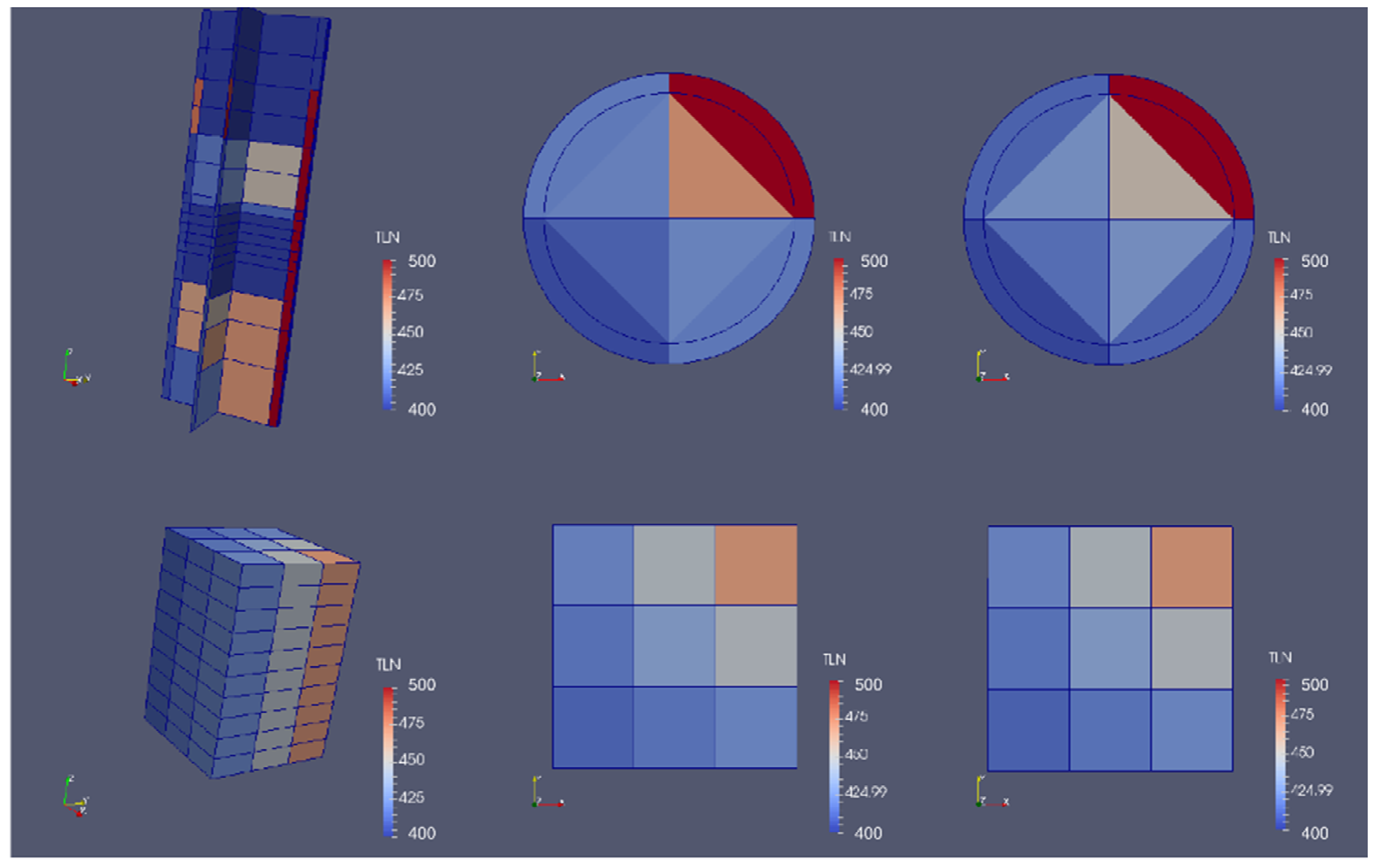
Figure 12 exhibits the qualitative distribution of the coolant temperature in the RPV and the core at the end of the transient. It can be observed that the coolant temperature of the cylindrical sectors of the CY-V corresponding to the loop-1 and of the Cartesian cells linked to it are hotter than the one of the other sectors/cells.

The coolant temperature distribution at the core inlet demonstrates that the coolant flows from the CY-V to the CA-V correctly. Similarly, the coolant temperature distribution at the core outlet shows that the coolant flow from the CA-V to the CY-V is passed from one VESSEL to the other properly. The roughly same temperature distribution at the CA-V inlet and outlet planes indicates weak coolant mixing in the core. However, we can see an obvious difference between the CY-V inlet and outlet planes. There at the CY-V outlet, the hot part is cooler and the cold part is hotter than that at the CY-V inlet. This indicates a considerable mixing in the core, which is not consistent with the conclusion from the CA-V analysis. This phenomenon is due to a “mixing” when the coolant flows from the coarse CY-V mesh to the fine CA-V mesh (from the lower plenum to the core) and then back to the CY-V mesh (from core to upper plenum). The intersections between fields in the different meshes introduce a sort of “averaging effect” into the system and thus cause a stronger mixing effect in the CY-V than that in the CA-V. This effect is now under study at KIT.

Another phenomenon we can observe from the figure is that the colors of the outer ring in the CY-V mesh intrude into the inner ring. These sorts of distortions are due to MED meshing limitations. The appearance has no concern with the physical aspects.

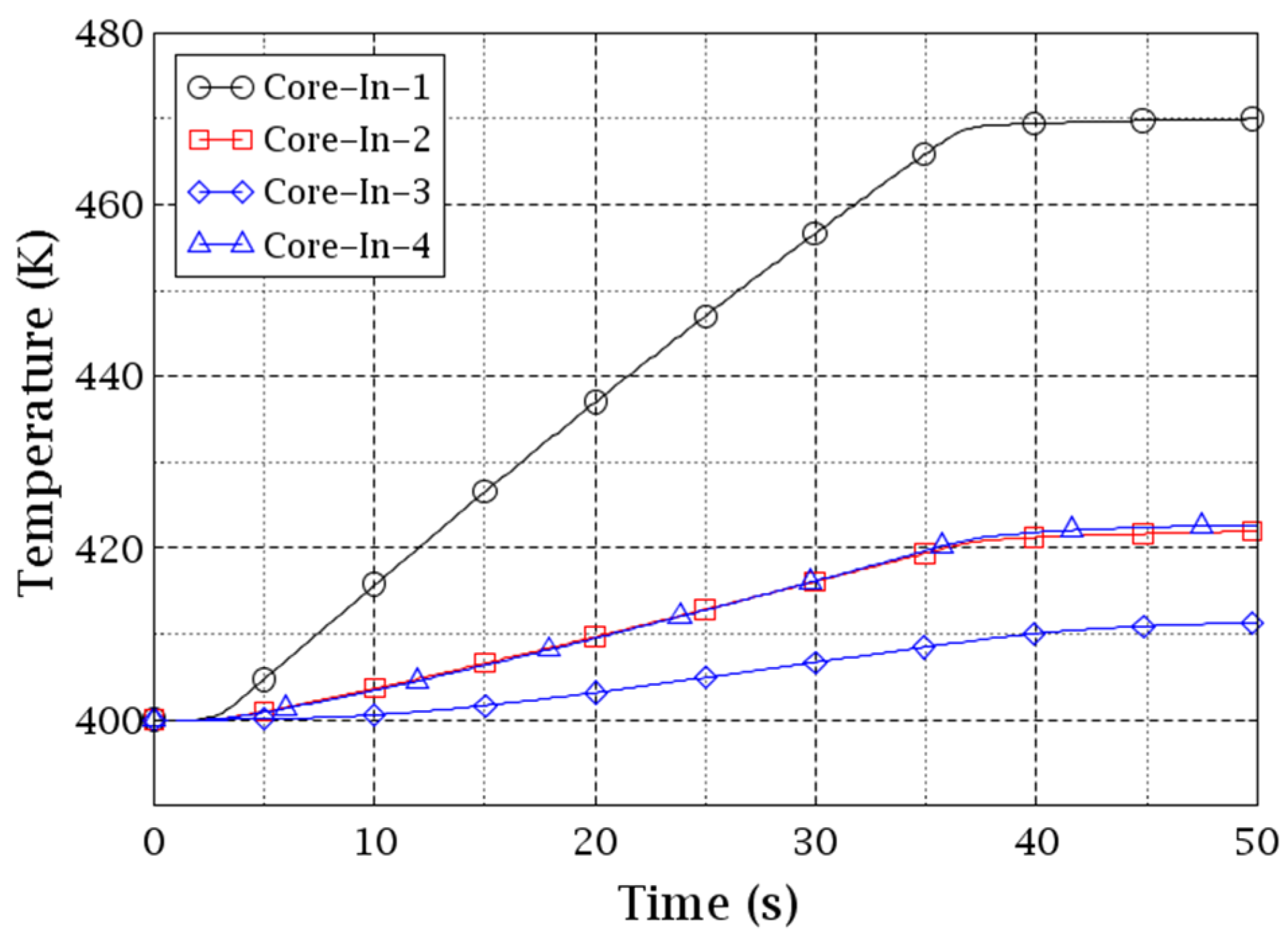
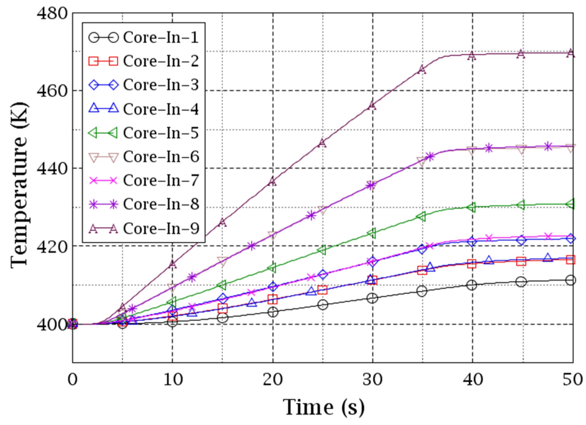
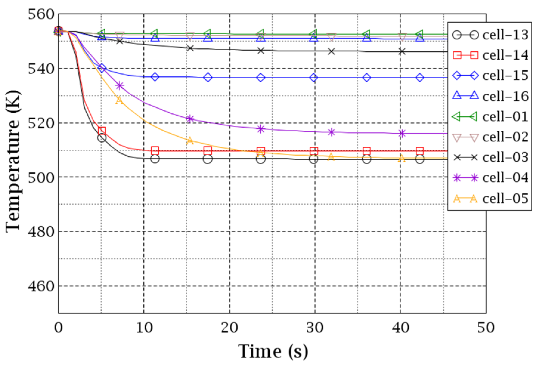
Figure 13 and Figure 14 exhibit the coolant temperature evolutions at the core inlet planes of the two VESSELs. Each curve represents an individual sector/cell on the planes. The former is for the CY-V (4 sectors) and the latter is for the CA-V (9 cells). The increase in the coolant temperature at the core inlet of sectors 2 and 4 is due to the coolant mixing taking place in the downcomer since these sectors are the neighbor sectors of sector 1 (hotter coolant).

Keeping in mind the cell indexing of the Cartesian VESSEL in Figure 10, it can be seen in Figure 14 that cell 9 is the hottest, cells 6 and 8 the second hottest, and cell 5 the third hottest. The coolant temperature of cell 9 is similar to the CY-V sector 1 while the coolant temperature of cells 6 and 8 are similar to sectors 2 and 4, see Figure 13 and Figure 14. The reason for it is the spatial correspondence of these cells and sectors which are automatically mapped with the MEDcoupling library. The transfer of physical fields between the two VESSELs is straightforward. On the contrary, cells 2/4/5/6/8 in the CA-V get the coolant from multiple cells of the CY-V. Thus, some kind of “averaging” effect would happen in those cells. Particularly, cells 6 and 8 of the CA-V mix the coolant from the hottest cell 1 and cell 2/4 of the CY-V. Therefore, their temperature curves in Figure 14 are in the middle of cell 1 and cell 3/7. Similarly, cells 2 and 4 of the CA-V mix the coolant from the coldest cell 3 and cell 4/2 of the CY-V. Therefore, their temperature curves in Figure 14 are in the middle of cell 3 and cell 3/7. Cell 5 is special because its coolant is from all of the 4 cells of CY-V.

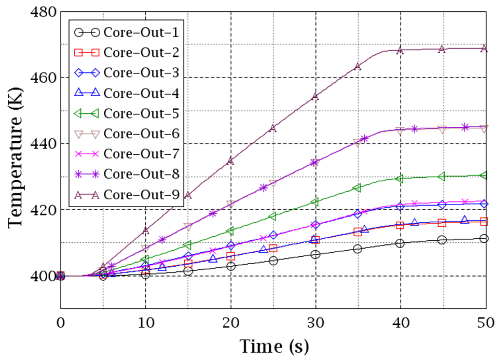
Figure 15 and Figure 16 show the coolant temperature evolutions at the core outlet planes of the two VESSELs. Each curve represents an individual cell/sector on the planes. The former is for the CA-V (9 cells) and the latter is for the CY-V (4 sectors). The minor difference between Figure 14 and Figure 16 indicates a weak coolant mixing effect in the core (by CA-V). However, a similar “averaging” effect happens when the coolant flows from the nine cells of CA-V to the four sectors of CY-V. The reason is that each of the four sectors in the CY-V gets the coolant from multiple cells of the CA-V. Particularly, sector 1 mixes the coolant from cell 5/6/8/9. Sector 2 mixes the coolant from the cell 4/5/7/8. Sector 3 mixes the coolant from the cell 1/2/4/5. Sector 4 mixes the coolant from the cell 2/3/5/6. Due to the two “averaging” effects happening on the core inlet/outlet as well as the coolant mixing in the core region, the temperature of the core flow-out coolant is more homogeneous than the core flow-in coolant in the CY-V.

In general, it can be stated that the coolant mixing in the downcomer is significant while the one inside the core is moderate.

4.2. The Coolant Mixing in the AP1000 Reactor

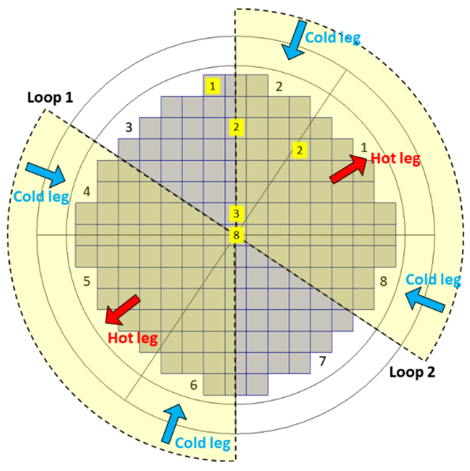
The configuration of the reactor and nodalization of the model were previously illustrated in Section 2.2 and Section 3. The RPV is represented by a CY-V and the core by a CA-V. The CY-V is nodalized to 8 azimuthal sectors and 2 radial rings while the CA-V is nodalized to 15 × 15 = 165 cells (each cell represents 1 fuel assembly), among which, 68 are dummy cells and 157 are real cells. Figure 17 only presents the real cells. Consequently, 456 additional PIPEs (as Junctions connecting the two VESSEL components) are constructed and inserted into the TRACE data structure automatically by the approach presented here. In total, 228 (1 × 96 + 2 × 56 + 3 × 4 + 8 × 1 = 228, Figure 17) of them are at the core inlet plane and 228 are at the core outlet plane. Figure 17 illustrates the quantitative distribution of the additional PIPEs from the point of the CA-V (for example, the yellow 8 means this cell connects to 8 CY-V sectors via 8 additional PIPEs as Junctions). Figure 17 gives the CY-V mesh as well. There, the sector indexes, the location of the loops, and the hot/cold legs are shown: the cold-legs (vessel inlet) of loop1 correspond to sectors 4 and 6 while the cold-legs of loop2 correspond to sectors 2 and 8. The hot-legs of loop1 and loop2 correspond to sectors 5 and 1.

First of all, a steady-state (SS) TRACE simulation is performed for an inlet mass flow rate of 3567 kg/s and coolant temperature of 553.7 K per loop (fixed as boundary conditions at the four FILL components). The outlet pressure is 15.45 MPa and is defined in the BREAK components. Afterward, a transient (TS) simulation is completed with the boundary conditions given in

Table 2. The boundary conditions during the transient on the AP1000 reactor.

	Inlet Mass Flow [kg/s]	Inlet Temperature [K]	Outlet Pressure [MPa]
Time	0~50 s	0~50 s	0~50 s
Loop 1	3658.0	453.7	15.45
Loop 2	3658.0	553.7	15.45

. The transient lasts for 50 s.

The transient is defined by decreasing the coolant temperature of the loop-1 from 553.7 to 543.7 K at the transient beginning. As a consequence, a coolant mixing will take place in the CY-V downcomer, in the CY-V lower plenum and the mixing pattern will be propagated to the CA-V core. After the final mixing in the CY-V upper plenum, the coolant will flow out of the RPV. The main question is to check if the automatic VESSEL-coupling is working properly for a coolant mixing problem. 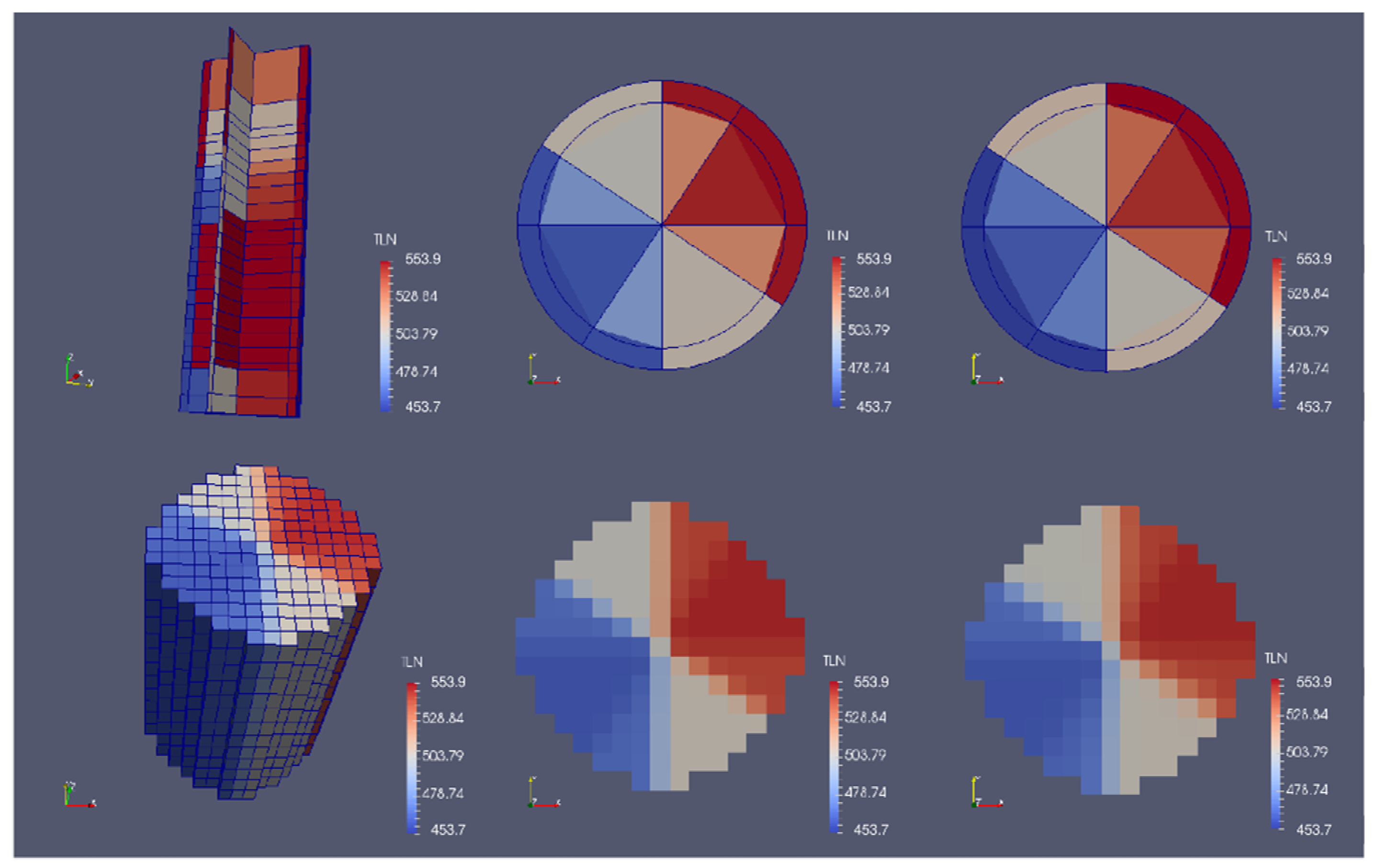Figure 18 exhibits the coolant temperature distributions in both the CY-V (top) and the CA-V (bottom) as shown by the new post-processing capability implemented in TRACE. It can be observed that the coolant temperature field of the loop-1 corresponding part in the CY-V and CA-V meshes is cooler than other parts. Particularly, the coolant temperature distribution at the core inlets implies that the coolant temperature was correctly transferred from the CY-V to the CA-V by the automatic VESSEL-coupling approach. The same conclusion can be drawn for the coolant temperature distribution at the core outlets.

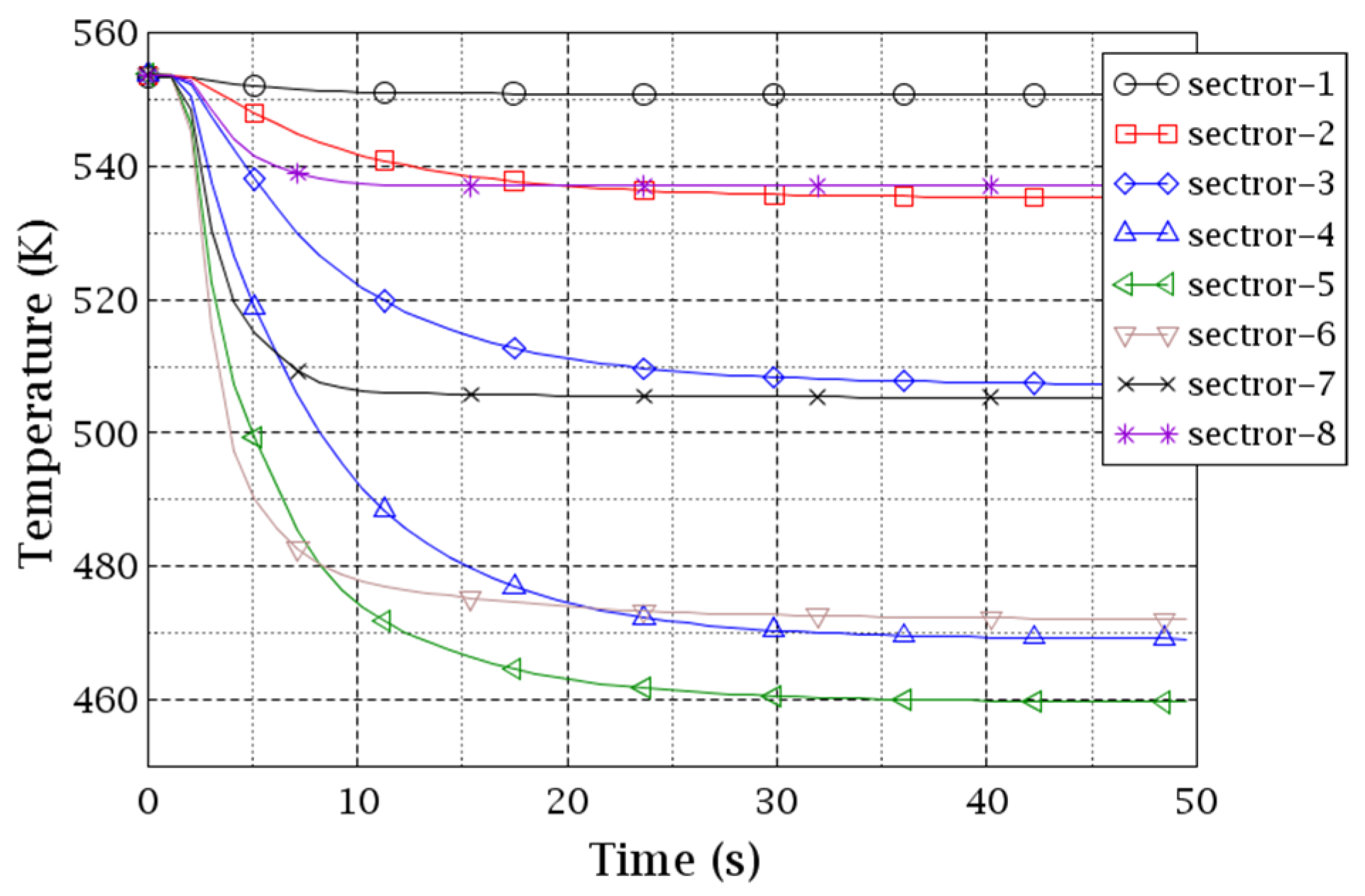
The coolant temperature evolution at the core inlet and outlet of the CY-V are plotted in Figure 19 and Figure 20, see Figure 17 for sector indexes. The coolant mixing in the downcomer and lower plenum can be observed if we examine the coolant temperature evolutions of sectors 3 and 7 which are the results of the coolant mixing between the coolant of the sectors 2 and 4 and the sectors 8 and 6.

This mixing pattern propagates from the CY-V lower plenum to the CA-V core at the core inlet and from the CA-V core to the CY-V upper plenum at the core outlet, where the mixing continues to happen in a moderate manner leading to a small reduction in the coolant temperature of the sectors 1, 2, and 8 at the core outlet compared to the ones at the core inlet. Contrary to it, the coolant temperature of sectors 4, 5, and 6 increases slightly at the core outlet compared to the core values at the core inlet.

In Figure 21, 16 representative cells of the CA-V are selected for the discussion of results from the CA-V side. To compare with the CY-V, 8 cells do not intersect with the CY-V sectors and their coolant comes from individual sectors. Eight cells intersect with the CY-V sectors and their coolant comes from two sectors. There, the correspondence of the CA-V cells with the CY-V sectors (and with the two loops) can be observed. The 16 representative cells are divided into two groups: the hot-part (loop2) and the cold-part (loop1).

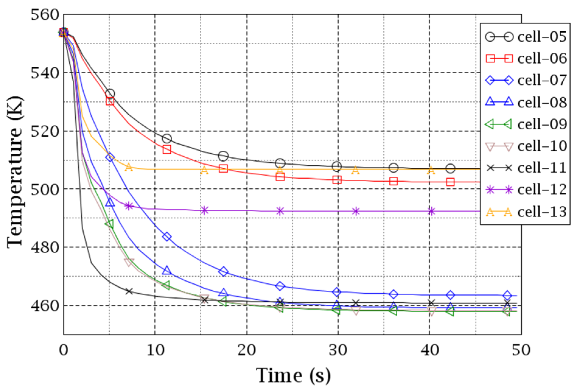
Figure 22 and Figure 23 show the coolant temperature evolutions of the hot-part and cold-part cells at the CA-V core inlet plane. Cells 1, 3, 5, 7, 9, 11, 13, and 15 have approximately identical trends as the corresponding sectors in the CY-V (1–8). Whereas some small differences can be observed due to the slight coolant mixing in the first level of the CA-V. Cells 2, 4, 6, 8, 10, 12, 14, and 16 are the CA-V cells that intersect with two CY-V sectors. The coolants from the two CY-V sectors mix when they flow into those CA-V cells. The mixing effect is inferred from Figure 22 and Figure 23, where the curves of the intersected CA-V cells located between their corresponding CY-V cells are exhibited.

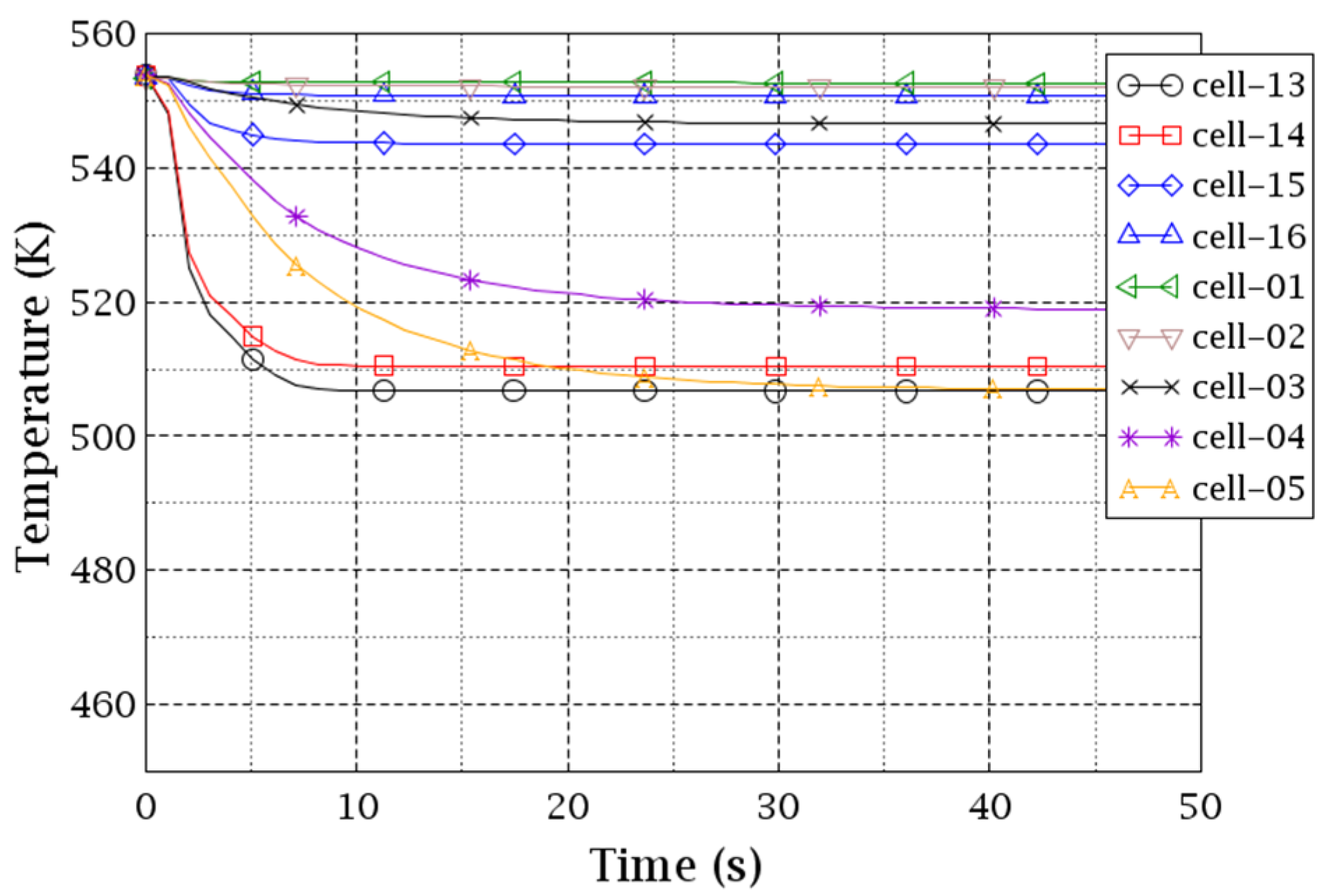
Figure 24 and Figure 25 give the coolant temperature evolution of the representative CA-V cells (Figure 21) at the core outlet. Most of the curves are approximately identical to that of the same cells at the core inlet except for cells 15, 4, 6, and 7. Thus, we can tell that the coolant mixing in the CA-V is relatively weak. At the core outlet plane, the coolant flows from CA-V to CY-V. There, each CY-V cell connects to a set of multiple CA-V cells. Compared with Figure 20, we can see a good agreement between the two distributions at the core outlets of the two VESSELs. If you look at sector 1 in the CY-V and cells 16, 1, and 2 in the CA-V, for example, the coolant temperature of sector 1 is slightly lower than the hottest cell 1 because colder coolant from boundary cells 2 and 16 contributes to sector 1 as well.

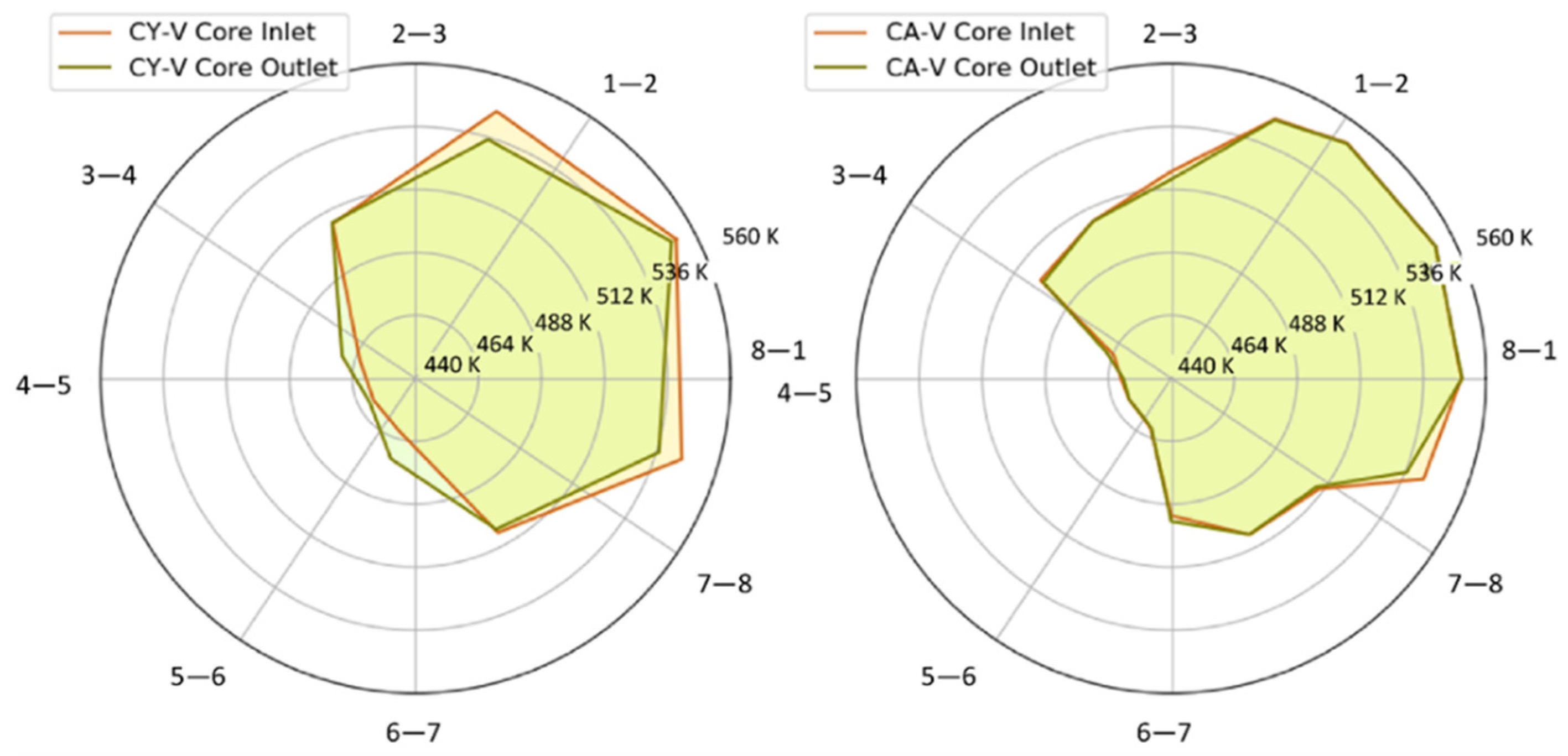
According to the analysis of the coolant mixing on the previous academic reactor, it can be inferred that the physical mixing and the “averaging effect” should both play a role in the AP1000 reactor when the coolant flows via the path of “CY-V to CA-V to CY-V”, because the meshes of the two VESSELs differ in spatial resolution and cell arrangement. Figure 26 plots the coolant temperature profile at the core inlet and outlet of the AP1000 CY-V and CA-V. There, the data points, as well as the theta coordinates are the ones of the CY-V sectors and the indexed CA-V cells that were given in Figure 21. The left subplot gives the field from CY-V, while the right gives the field from CA-V. For both subplots, the orange curve and block represent the field at the core inlet, while dark green represents the field at the core outlet.

We can see an obvious shrinkage of the hot part (between the lines 1–2 and 8–1) and an expansion of the cold part (between the lines 3–4 and 6–7) when comparing the temperature profile at the CY-V core outlet to that at the CY-V core inlet. The more eccentric the block is on this radar map, the more inhomogeneously the temperature field distributes at the core inlet or outlet planes.

Globally, the temperature band at the outlet moves closer to the center, which indicates a flatter coolant temperature distribution at the core outlet. However, this sort of shrinkage, expansion, and movement is not that noticeable in Figure 26 (right). This leads to the conclusion that the coolant mixing in the CA-V is weak (consistent with the analysis in Figure 22, Figure 23, Figure 24 and Figure 25). Thus, we can conclude that the “averaging effect” contributes to the temperature flatting that is observed in Figure 26 (left). This effect is still under study at present. Nevertheless, the result from the AP1000 reactor demonstrates the adequacy and efficiency of the automatic VESSEL-coupling approach presented and discussed here.

5. Conclusions

The paper discussed the development of an innovative method for the automatic coupling of two different 3D components of the TRACE code, i.e., the Cylindrical VESSEL (CY-V) and Cartesian VESSEL (CA-V) for the improved simulation of the 3D phenomena in the core and Reactor Pressure Vessel (RPV) of a Nuclear Power Plant (NPP). Thanks to the functionalities of the MEDcoupling library, the users do not need to manually define the numerous junctions of the VESSEL-Junction (VJ) component in SNAP to connect the core inlet and outlet of the CA-V core with the CA-V RPV. Aside from the automation functionality, the Junction definition and the calculation of relevant Thermal-Hydraulic (TH) parameters are more precise using this approach. The new capabilities of TRACE were demonstrated by analyzing two coolant mixing problems in the RPV of a generic four-loop Light Water Reactor (LWR) and the AP-1000 reactor. The results indicate the mixing inside the downcomer and core. The quantitative evolution of the mixing pattern shows that the mixing inside the core is less than the one in the downcomer and that the developed approach works fine. Last but not least, the predictions demonstrated that the data transfer at the core inlet and outlet between the two VESSELs is working properly. In future investigations, the root causes for the “averaging effect” due to the mesh differences will be investigated. Furthermore, the existence of more than one VESSEL to represent the RPV, e.g., of a Small Modular Reactor (SMR), will be implemented.

References

1. Bajorek, S.M.; Bernard, M.; Gingrich, C.; Hoxie, C.L.; Ireland, A.; Kelly, J.; Mahaffy, J.; Murray, C.; Spore, J.; Staudenmeier, J.; et al. Development, Validation and Assessment of the TRACE Thermal-Hydraulics System Code. In Proceedings of the 16th International Topical Meeting on Nuclear Reactor Thermal Hydraulics (NURETH-16), Chicago, IL, USA, 30 August–4 September 2015; pp. 8265–8278. [Google Scholar]
2. Idaho National Laboratory (INL). RELAP5-3D Home. Available online: https://relap53d.inl.gov/SitePages/Home.aspx (accessed on 21 March 2022).
3. Applied Programming Technology. Symbolic Nuclear Analysis Package. Available online: https://www.snaphome.com/snap/index.jsp (accessed on 21 March 2022).
4. Emonot, P.; Souyri, A.; Gandrille, J.; Barre, F. CATHARE-3: A new system code for thermal-hydraulics in the context of the NEPTUNE project. Nucl. Eng. Des. 2011, 241, 4476–4481. [Google Scholar] [CrossRef]
5. CEA. GUITHARE—Graphical User Interface for CATHARE. Available online: https://cathare.cea.fr/Pages/CATHARE/GUITHARE.aspx (accessed on 16 May 2022).
6. CEA. CATHARE Thermal-Hydraulic Simulation of Multiphase Flow Dynamics—R&D. Available online: https://cathare.cea.fr/Pages/CATHARE/R_and_D.aspx (accessed on 21 March 2022).
7. Prea, R.; Figerou, V.; Mekkas, A.; Ruby, A. CATHARE-3: A First Computation of a 3-inch Break Loss-of-Coolant Accident using both Cartesian and Cylindrical 3D-meshes Modeling of a PWR Vessel. In Proceedings of the NURETH-17, Xi’an, China, 3–8 September 2017. [Google Scholar]
8. Open Cascade; CEA; EDF. MEDCoupling Developer’s Guide. Available online: http://docs.salome-platform.org/latest/dev/MEDCoupling/developer/index.html (accessed on 21 March 2022).
9. Zhang, K. The Multiscale Thermal-hydraulic Simulation for Nuclear Reactors: A Classification of the Coupling Approaches and a Review of the Coupled Codes. Int. J. Energy Res. 2020, 44, 3295–3315. [Google Scholar] [CrossRef] [Green Version]
10. Zhang, V.K.; Sanchez Espinoza, H.; Stieglitz, R. Implementation of the System Thermal-Hydraulic code TRACE into SALOME Platform for Multi-Scale Coupling. In Proceedings of the 50th Annual Meeting on Nuclear Technology AMNT, Berlin, Germany, 7–8 May 2019. [Google Scholar]
11. Zhang, K.; Muñoz, A.C.; Sanchez-Espinoza, V.H. Development and Verification of the Coupled Thermal–Hydraulic Code—TRACE/SCF based on the ICoCo Interface and the SALOME Platform. Ann. Nucl. Energy 2021, 155, 108169. [Google Scholar] [CrossRef]
12. Zhang, K.; Zhang, X.; Sanchez-Espinoza, V.; Stieglitz, R. Development of the Coupled Code—TRACE/TrioCFD based on ICoCo for Simulation of Nuclear Power Systems and its Validation against the VVER-1000 Coolant-Mixing Benchmark. Nucl. Eng. Des. 2020, 362, 110602. [Google Scholar] [CrossRef]
Figure 1. The CY-V (a) and CA-V (b) components.
Energies 15 04384 g001
Figure 2. The diagram of the primary circuit of AP1000.
Energies 15 04384 g002
Figure 3. The AP1000 model demonstrates the multi-vessel coupling rules.
Energies 15 04384 g003
Figure 4. The definition panel of VJ components in SNAP.
Energies 15 04384 g004
Figure 5. The axial cross-sections of the VESSELs and the intersection of the cells. (a) The CY-V; (b) intersections of the cells; (c) the CA-V.
Energies 15 04384 g005
Figure 6. The meshes of the CY-V and CA-V (from left to right, from top to bottom: 3D body mesh/3D surface mesh/2D mesh of CY-V, 2D mesh/3D body mesh/3D surface mesh of CA-V).
Energies 15 04384 g006
Figure 7. The AP1000 model uses the new method to handle the new multi-vessel coupling.
Energies 15 04384 g007
Figure 8. The main procedures during a multi-vessel coupling process.
Energies 15 04384 g008
Figure 9. The complementary PIPE components between the two VESSELs.
Energies 15 04384 g009
Figure 10. Nodalization of the CY-V (left) and the CA-V (right).
Energies 15 04384 g010
Figure 11. The quantitative distribution of the additional PIPEs at the core inlet/outlet planes.
Energies 15 04384 g011
Figure 12. The coolant temperature distributions in the CY-V and CA-V (from left to right, from top to bottom: 3D field/2D field at the core inlet/2D field at the core outlet of CY-V, 3D field/2D field at the core inlet/2D field at the core outlet of CA-V).
Energies 15 04384 g012
Figure 13. Evolution of the coolant temperature distribution at the core inlet CY-V (cell index is from Figure 10).
Energies 15 04384 g013
Figure 14. Evolution of the coolant temperature distribution at the core inlet CA-V (cell index is from Figure 10).
Energies 15 04384 g014
Figure 15. Evolution of the coolant temperature distribution at the core outlet CY-V (cell index is from Figure 10).
Energies 15 04384 g015
Figure 16. Evolution of the coolant temperature distribution at the core outlet CA-V (cell index is from Figure 10).
Energies 15 04384 g016
Figure 17. The quantitative distribution of the additional PIPEs at the core inlet/outlet planes of the AP1000 reactor.
Energies 15 04384 g017
Figure 18. The coolant temperature distributions in the CY-V and CA-V of the AP1000 reactor (from left to right, from top to bottom: 3D field/2D field at the core inlet/2D field at the core outlet of CY-V, 3D field/2D field at the core inlet/2D field at the core outlet of CA-V).
Energies 15 04384 g018
Figure 19. Evolution of the coolant temperature distribution at the core inlet of the AP1000 reactor CY-V (cell index is from Figure 17).
Energies 15 04384 g019
Figure 20. Evolution of the coolant temperature distribution at the core outlet of the AP1000 reactor CY-V (cell index is from Figure 17).
Energies 15 04384 g020
Figure 21. The AP1000 selected cells (assemblies in CA-V) whose coolant temperature evolutions are studied.
Energies 15 04384 g021
Figure 22. Evolution of the coolant temperature distribution at the core inlet of the AP1000 reactor CA-V hot-part (cell index is from Figure 21).
Energies 15 04384 g022
Figure 23. Evolution of the coolant temperature distribution at the core inlet of the AP1000 reactor CA-V cold-part (cell index is from Figure 21).
Energies 15 04384 g023
Figure 24. Evolution of the coolant temperature distribution at the core outlet of the AP1000 reactor CA-V hot-part (cell index is from Figure 21).
Energies 15 04384 g024
Figure 25. Evolution of the coolant temperature distribution at the core outlet of the AP1000 reactor CA-V cold-part (cell index is from Figure 21).
Energies 15 04384 g025
Figure 26. The coolant temperature profile at the core inlet and outlet of the AP1000 CY-V and CA-V (data from the CY-V_sectors and indexed CA-V_cells in Figure 21).
Energies 15 04384 g026