
A Well-Overflow Prediction Algorithm Based on Semi-Supervised Learning


Abstract
:1. Introduction
2. Related Work
2.1. Semi-Supervised Learning
- Smoothing hypothesis.
- When two samples are very close in the high-density data region, their class labels are likely to be the same; on the contrary, when the low-density data regions divide the two samples, they are likely to have different class labels.
- Clustering hypothesis.
- When two samples belong to the same cluster, their class labels are probably the same. This hypothesis is also named as low-density separation hypothesis, which means that the classification decision surface should be located in the low-density data region instead of the high-density data area. The decision surface should not divide the samples from the same high-density data area into both sides of the surface.
- Manifold hypothesis.
- On the one hand, in high-dimensional space, the data volume increases exponentially as the dimension increases, so it is difficult to estimate the real data distribution. On the other hand, if the input data is on some low-dimensional manifold, a low-dimensional representation could be found by unlabeled data, and then the simplified task will be fulfilled with labeled data. Therefore, the manifold hypothesis maps the high-dimensional data to the low-dimensional manifold, and if the two samples are located in the local neighborhood of the low-dimensional manifold, their class labels are likely to be the same.
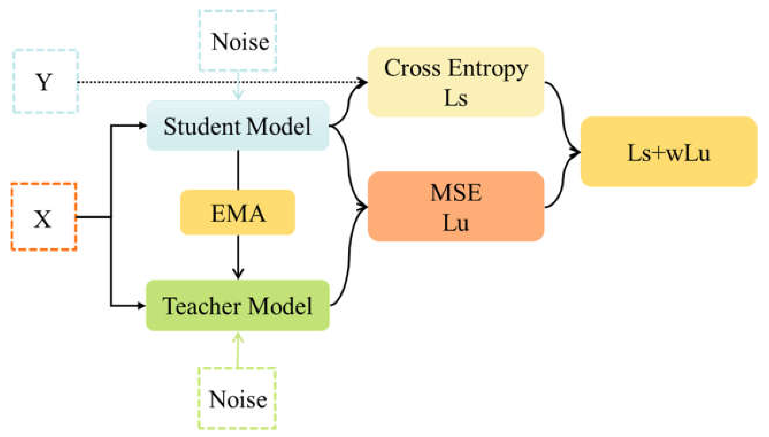
2.2. Mean Teacher Algorithm
| Algorithm 1. Mean Teacher learning algorithm. |
|
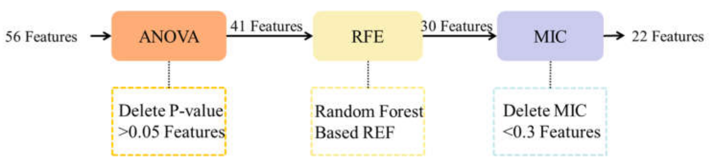
3. Dataset and Feature Selection
4. Methodology
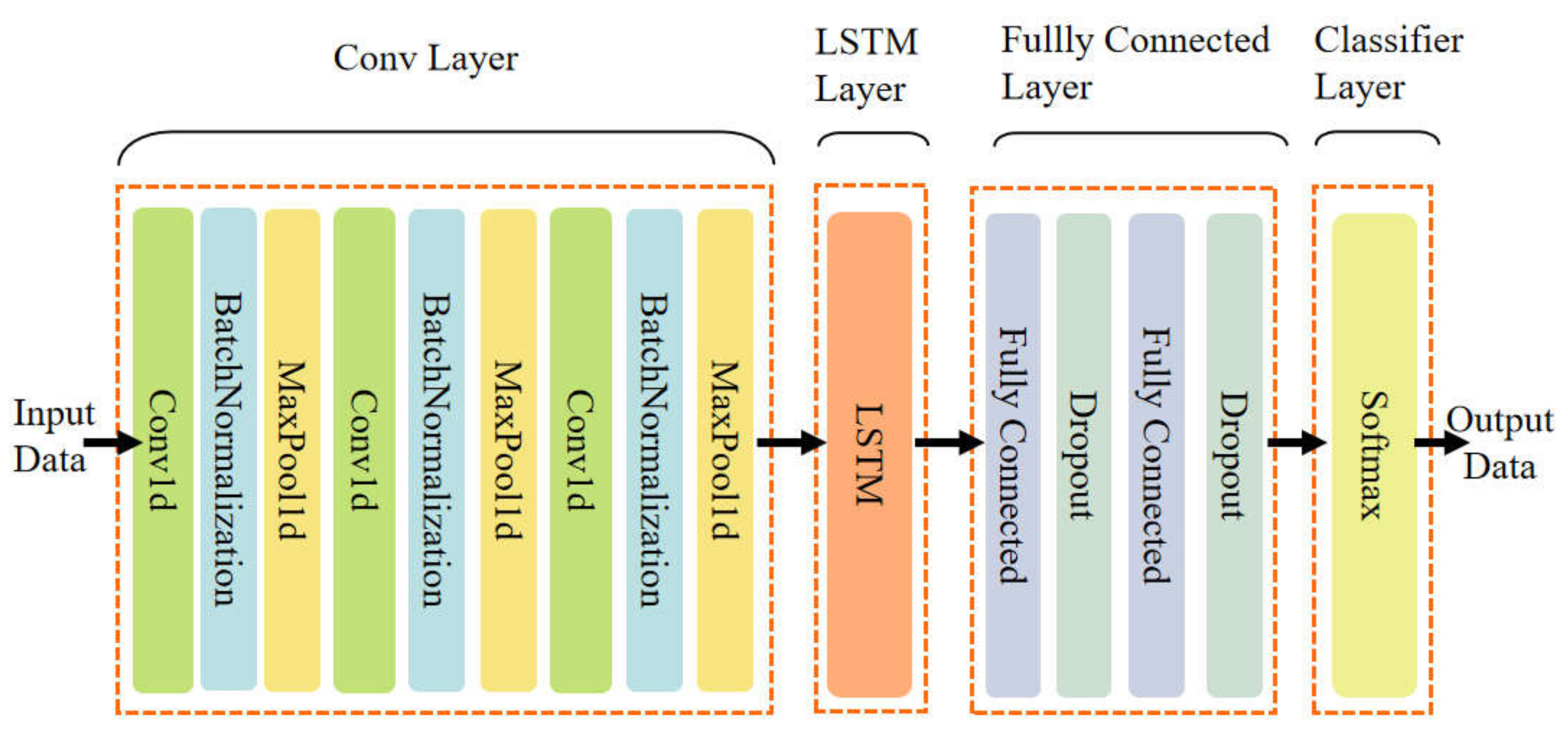
4.1. The Prediction Model
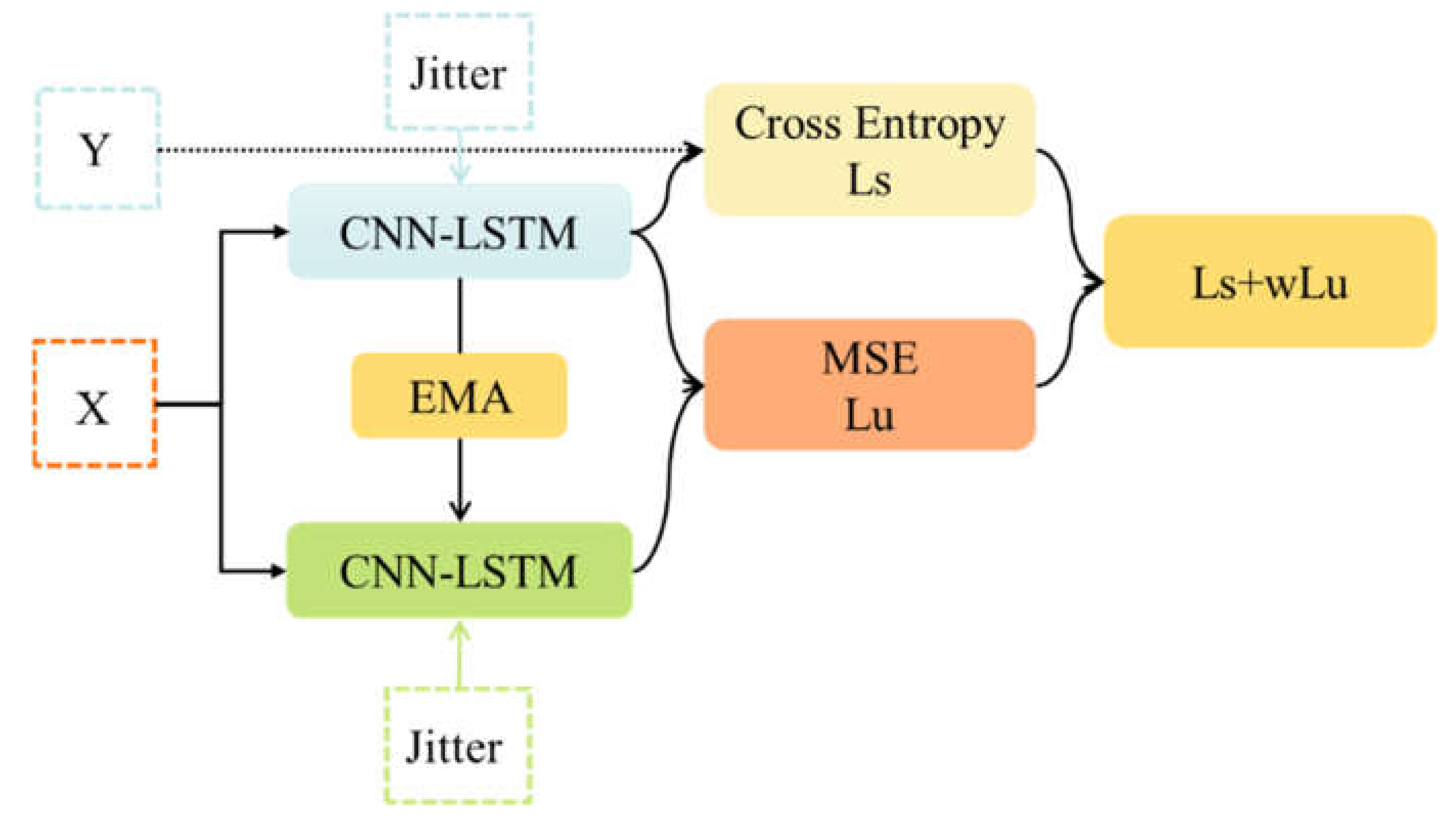
4.2. Construction of Semi-Supervised Framework
5. Results
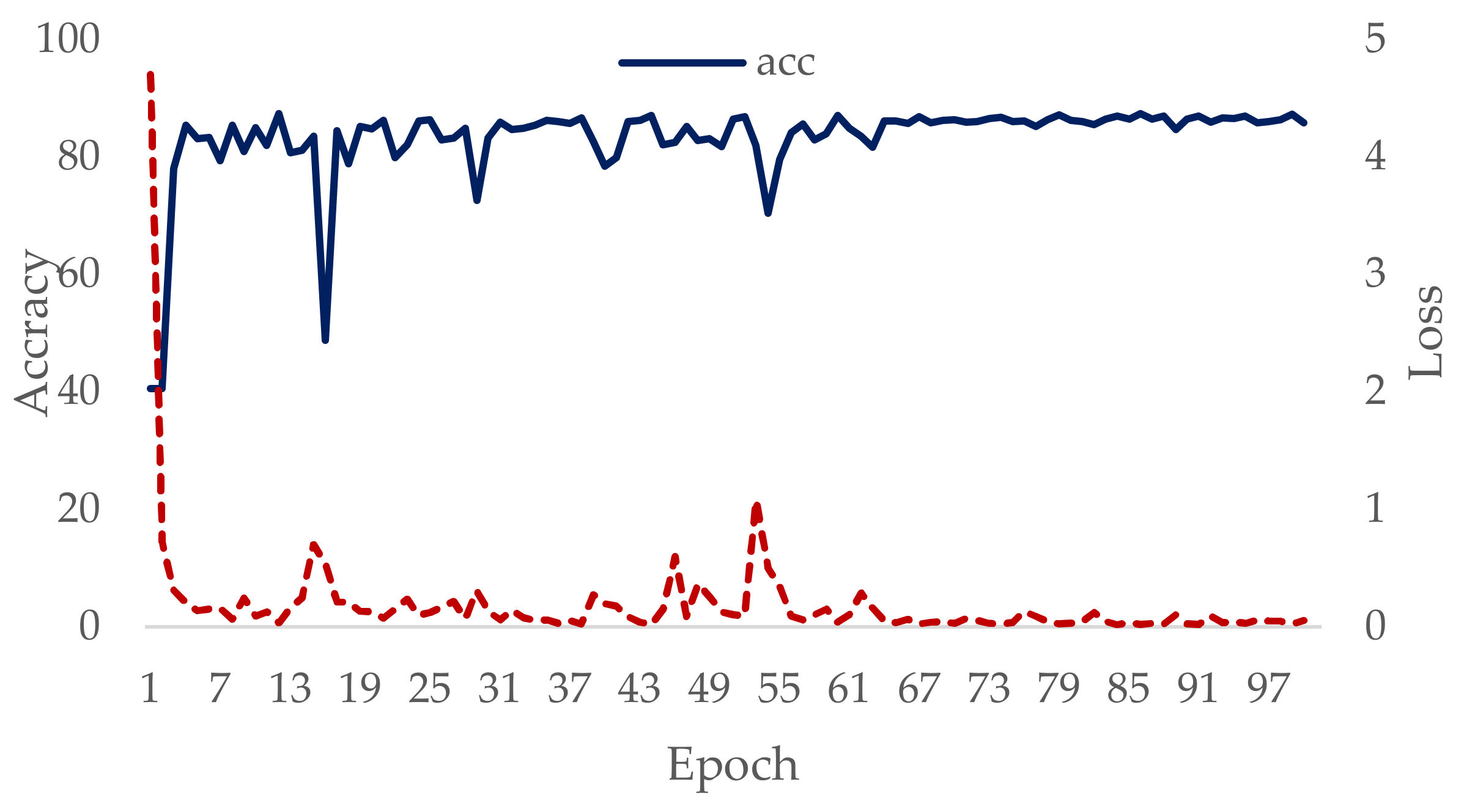
5.1. Model Training
5.2. Model Results
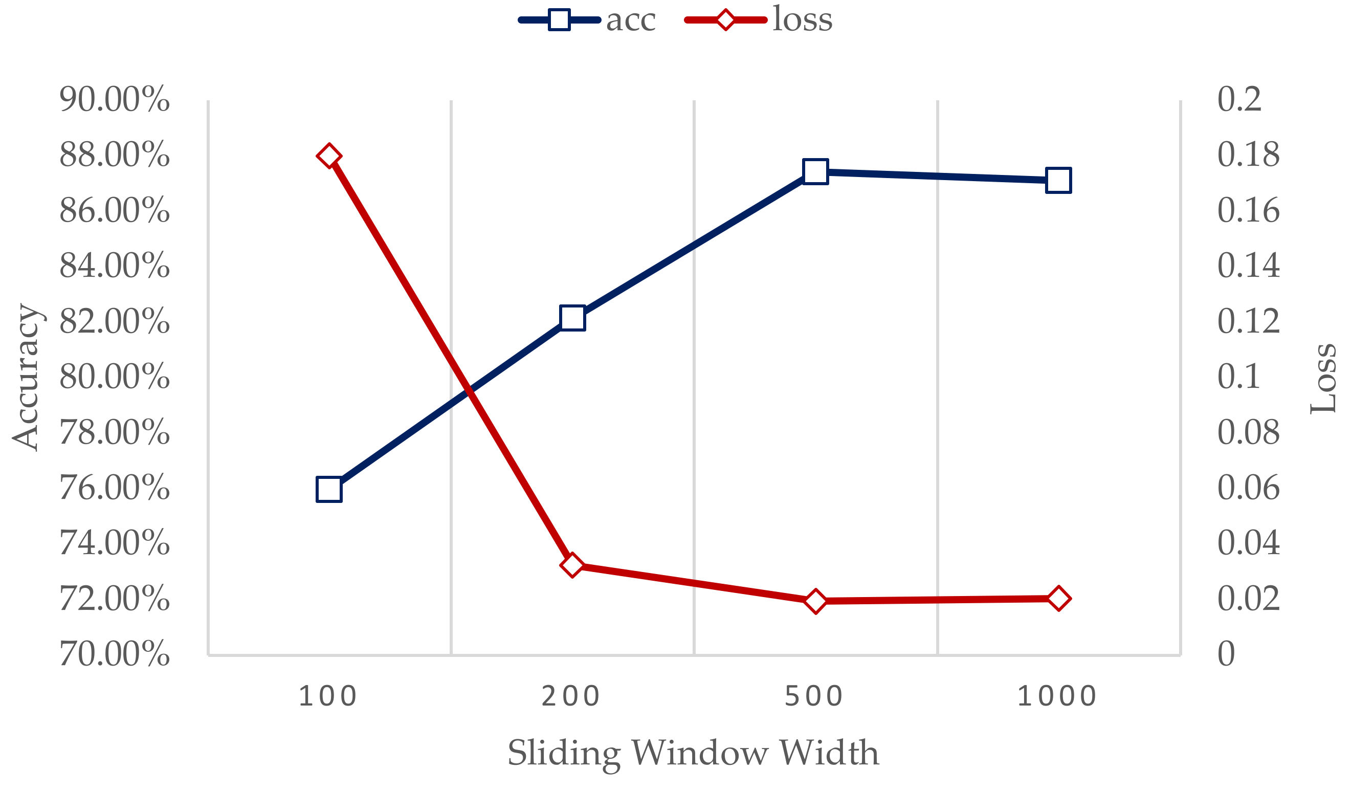
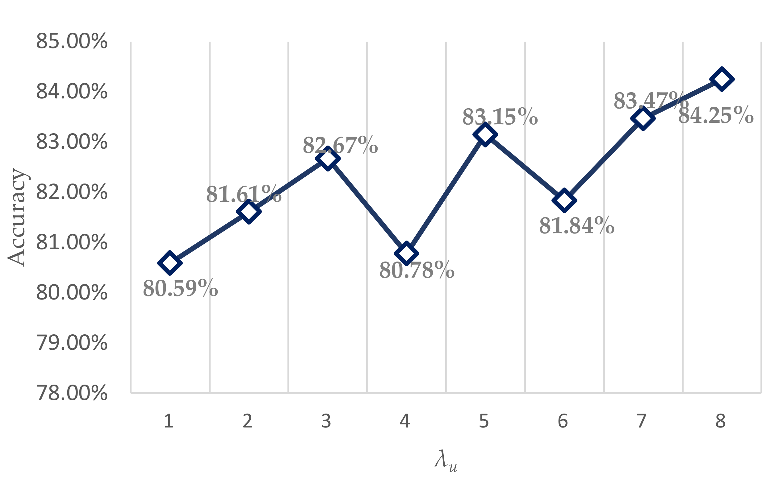
5.3. Sensitivity Analysis
6. Conclusions
Supplementary Materials
Author Contributions
Funding
Informed Consent Statement
Data Availability Statement
Conflicts of Interest
References
- Hargreaves, D.; Jardine, S.; Jeffryes, B. Early Kick Detection for Deepwater Drilling: New Probabilistic Methods Applied in the Field. In Proceedings of the SPE Annual Technical Conference and Exhibition, New Orleans, LA, USA, 30 September–3 October 2001; OnePetro: Richardson, TX, USA, 2001. [Google Scholar]
- Wang, X.L.; Lian, X.; Yao, L. Fault Diagnosis of Drilling Process Based on Rough Set and Support Vector Machine. Adv. Mater. Res. 2013, 709, 266–272. Available online: https://www.scientific.net/AMR.709.266 (accessed on 4 May 2022).
- Lind, Y.B.; Kabirova, A.R. Artificial Neural Networks in Drilling Troubles Prediction. In Proceedings of the SPE Russian Oil and Gas Exploration & Production Technical Conference and Exhibition, Moscow, Russia, 14–16 October 2014; OnePetro: Richardson, TX, USA, 2014. [Google Scholar]
- Li, X.; Liang, H.; Wang, X. Overflow Prediction Method Using Fuzzy Expert System. Int. Core J. Eng. 2015, 7, 58–64. [Google Scholar]
- Liang, H.; Zou, J.; Li, Z.; Khan, M.J.; Lu, Y. Dynamic evaluation of drilling leakage risk based on fuzzy theory and PSO-SVR algorithm. Future Gener. Comput. Syst. 2019, 95, 454–466. [Google Scholar] [CrossRef]
- Liang, H.; Zou, J.; Liang, W. An early intelligent diagnosis model for drilling overflow based on GA–BP algorithm. Clust. Comput. 2019, 22, 10649–10668. [Google Scholar] [CrossRef]
- Haibo, L.; Zhi, W. Application of an intelligent early-warning method based on DBSCAN clustering for drilling overflow accident. Clust. Comput. 2019, 22, 12599–12608. [Google Scholar] [CrossRef]
- Zhu, Q.; Wang, Z.; Huang, J. Stuck Pipe Incidents Prediction Based On Data Analysis. In Proceedings of the SPE Gas & Oil Technology Showcase and Conference, Dubai, United Arab Emirates, 21–23 October 2019; OnePetro: Richardson, TX, USA, 2019. [Google Scholar]
- Borozdin, S.; Dmitrievsky, A.; Eremin, N.; Arkhipov, A.; Sboev, A.; Chashchina-Semenova, O.; Fitzner, L.; Safarova, E. Drilling Problems Forecast System Based on Neural Network. In Proceedings of the SPE Annual Caspian Technical Conference, Online, 21–22 October 2020; OnePetro: Richardson, TX, USA, 2020. [Google Scholar]
- Sabah, M.; Mehrad, M.; Ashrafi, S.B.; Wood, D.A.; Fathi, S. Hybrid machine learning algorithms to enhance lost-circulation prediction and management in the Marun oil field. J. Pet. Sci. Eng. 2021, 198, 108125. [Google Scholar] [CrossRef]
- Liu, Z.; Ma, Q.; Cai, B.; Liu, Y.; Zheng, C. Risk assessment on deepwater drilling well control based on dynamic Bayesian network. Process Saf. Environ. Prot. 2021, 149, 643–654. [Google Scholar] [CrossRef]
- Yin, B.; Li, B.; Liu, G.; Wang, Z.; Sun, B. Quantitative risk analysis of offshore well blowout using bayesian network. Saf. Sci. 2021, 135, 105080. [Google Scholar] [CrossRef]
- Liang, H.; Han, H.; Ni, P.; Jiang, Y. Overflow warning and remote monitoring technology based on improved random forest. Neural Comput. Appl. 2021, 33, 4027–4040. [Google Scholar] [CrossRef]
- Wang, K.; Liu, Y.; Li, P. Recognition method of drilling conditions based on support vector machine. In Proceedings of the 2022 IEEE 2nd International Conference on Power, Electronics and Computer Applications (ICPECA), Shenyang, China, 21–23 January 2022; IEEE: Piscataway, NJ, USA, 2022; pp. 233–237. [Google Scholar]
- Ouali, Y.; Hudelot, C.; Tami, M. An Overview of Deep Semi-Supervised Learning. arXiv 2020, arXiv:2006.05278. [Google Scholar]
- Tarvainen, A.; Valpola, H. Mean teachers are better role models: Weight-averaged consistency targets improve semi-supervised deep learning results. In Proceedings of the 31st Conference on Neural Information Processing Systems (NIPS 2017), Long Beach, CA, USA, 4 December 2017; Curran Associates, Inc.: New York, NY, USA, 2017; Volume 30. [Google Scholar]
- Ge, R.; Zhou, M.; Luo, Y.; Meng, Q.; Mai, G.; Ma, D.; Wang, G.; Zhou, F. McTwo: A two-step feature selection algorithm based on maximal information coefficient. BMC Bioinform. 2016, 17, 142. [Google Scholar] [CrossRef] [PubMed] [Green Version]
- Wen, Q.; Sun, L.; Yang, F.; Song, X.; Gao, J.; Wang, X.; Xu, H. Time Series Data Augmentation for Deep Learning: A Survey. arXiv 2021, 5, 4653–4660. [Google Scholar]
- Um, T.T.; Pfister, F.M.J.; Pichler, D.; Endo, S.; Lang, M.; Hirche, S.; Fietzek, U.; Kulić, D. Data augmentation of wearable sensor data for parkinson’s disease monitoring using convolutional neural networks. In Proceedings of the 19th ACM International Conference on Multimodal Interaction, Glasgow, UK, 13–17 November 2017; Association for Computing Machinery: New York, NY, USA, 2017; pp. 216–220. [Google Scholar]
- Fu, J.; Liu, W.; Han, X.; Li, F. CNN-LSTM Fusion Network Based Deep Learning Method for Early Prediction of Overflow. China Pet. Mach. 2021, 49, 16–22. [Google Scholar] [CrossRef]
- Lee, D.-H. Pseudo-label: The simple and efficient semi-supervised learning method for deep neural networks. In Proceedings of the ICML 2013 Workshop: Challenges in Representation Learning, Atlanta, GA, USA, 21 June 2013; ICML: San Diego, CA, USA, 2013; pp. 1–6. [Google Scholar]


| No. | Time | Total Number | Samples before Overflow | Overflow Samples |
|---|---|---|---|---|
| 1 | 10.11 10:53–10.11 11:52 | 3187 | 2608 | 579 |
| 2 | 10.11 9:30–10.11 10:53 | 4392 | 3169 | 1223 |
| 3 | 10.11 10:53–10.11 11:52 | 3283 | 2645 | 638 |
| 4 | 10.29 6:14–10.29 7:55 | 5375 | 3221 | 2154 |
| 5 | 10.29 0:45–10.29 2:15 | 4800 | 3172 | 1628 |
| 6 | 10.28 16:39–10.28 18:14 | 4973 | 3867 | 1106 |
| 7 | 10.28 12:41–10.28 14:13 | 4834 | 2724 | 2110 |
| 8 | 10.24 1:56–10.24 2:25 | 1595 | 956 | 639 |
| 9 | 10.24 0:28–10.24 1:55 | 4663 | 3181 | 1482 |
| 10 | 10.22 23:49–10.23 0:50 | 6524 | 3180 | 3344 |
| No. | Feature Name | No. | Feature Name |
|---|---|---|---|
| 1 | Drilling Time (min/m) | 12 | Inlet Temperature (°C) |
| 2 | Bit Pressure (KN) | 13 | Outlet Temperature (°C) |
| 3 | Hook Load (KN) | 14 | Total Hydrocarbons (%) |
| 4 | Torque (KN·m) | 15 | PWD Vertical Depth (m) |
| 5 | Hook Position (m) | 16 | PWD Annulus Pressure (MPa) |
| 6 | Hook Speed (m/s) | 17 | PWD Angle of Inclination (°) |
| 7 | Standpipe Pressure (MPa) | 18 | PWD Direction (°) |
| 8 | Totle Pump Stroke (SPM) | 19 | C2 (%) |
| 9 | Mud Tanks Volume (m3) | 20 | Wellhead Pressure (MPa) |
| 10 | Circulating Pressure Loss (MPa) | 21 | Outlet Flow (L/s) |
| 11 | Lag Time (min) | 22 | Inlet Flow (L/s) |
| Parameter | 50 Labels | 200 Labels | 1000 Labels | All Labels |
|---|---|---|---|---|
| Batch_Size (N + ) | 60 | 300 | 600 | 200 |
| Label_Batch_Size (N) | 10 | 50 | 100 | 200 |
| Epoch | 100 | 100 | 100 | 300 |
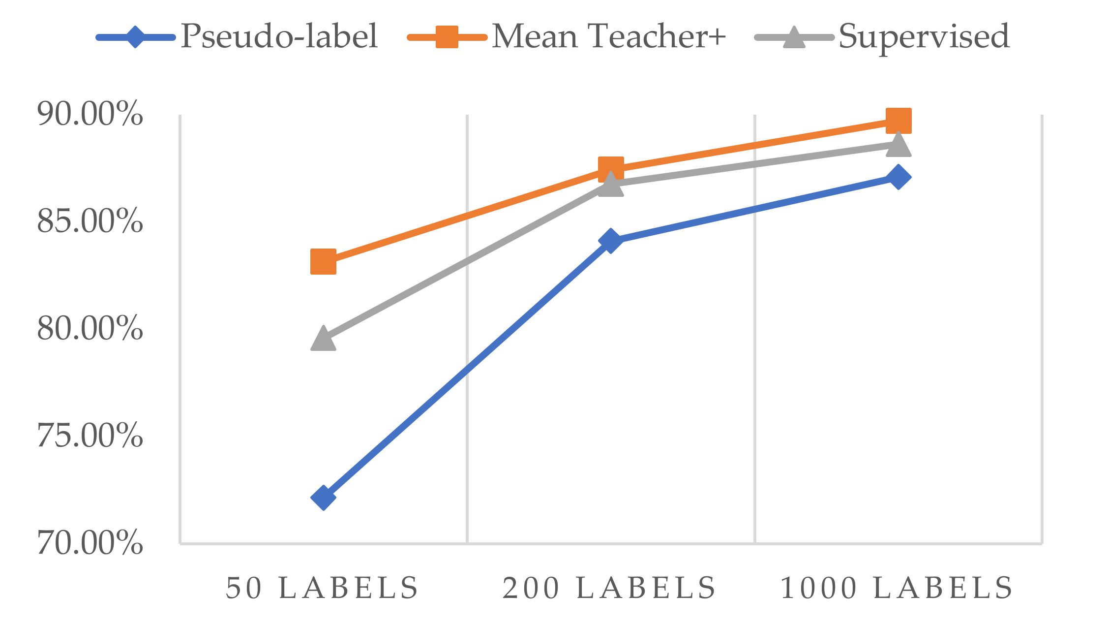
| Method | 50 Labels | 200 Labels | 1000 Labels | All Labels |
|---|---|---|---|---|
| Pseudo-label | 72.17% | 84.13% | 87.10% | - |
| Mean Teacher+ | 83.15% | 87.43% | 89.70% | - |
| Supervised | 79.59% | 86.77% | 88.62% | 89.90% |
| Method | Precision | Recall | F1 |
|---|---|---|---|
| SVM | 0.9679 | 0.6047 | 0.7443 |
| Random Forest | 0.9876 | 0.6220 | 0.7632 |
| LightGBM | 0.6246 | 0.6827 | 0.6523 |
| XGBoost | 0.9504 | 0.5039 | 0.6586 |
| CNN-LSTM | 0.7851 | 0.8064 | 0.7956 |
| MeanTeacher− | 0.8746 | 0.7527 | 0.8091 |
| MeanTeacher | 0.8804 | 0.7539 | 0.8123 |
| MeanTeacher+ | 0.9154 | 0.7467 | 0.8225 |
Publisher’s Note: MDPI stays neutral with regard to jurisdictional claims in published maps and institutional affiliations. |
© 2022 by the authors. Licensee MDPI, Basel, Switzerland. This article is an open access article distributed under the terms and conditions of the Creative Commons Attribution (CC BY) license (https://creativecommons.org/licenses/by/4.0/).
Share and Cite
Liu, W.; Fu, J.; Liang, Y.; Cao, M.; Han, X. A Well-Overflow Prediction Algorithm Based on Semi-Supervised Learning. Energies 2022, 15, 4324. https://doi.org/10.3390/en15124324
Liu W, Fu J, Liang Y, Cao M, Han X. A Well-Overflow Prediction Algorithm Based on Semi-Supervised Learning. Energies. 2022; 15(12):4324. https://doi.org/10.3390/en15124324
Chicago/Turabian StyleLiu, Wei, Jiasheng Fu, Yanchun Liang, Mengchen Cao, and Xiaosong Han. 2022. "A Well-Overflow Prediction Algorithm Based on Semi-Supervised Learning" Energies 15, no. 12: 4324. https://doi.org/10.3390/en15124324
APA StyleLiu, W., Fu, J., Liang, Y., Cao, M., & Han, X. (2022). A Well-Overflow Prediction Algorithm Based on Semi-Supervised Learning. Energies, 15(12), 4324. https://doi.org/10.3390/en15124324