Abstract
An ultracapacitor State-of-Charge (SOC) fusion estimation method for electric vehicles under variable temperature environment is proposed in this paper. Firstly, Thevenin model is selected as the ultracapacitor model. Then, genetic algorithm (GA) is adopted to identify the ultracapacitor model parameters at different temperatures (−10 °C, 10 °C, 25 °C and 40 °C). Secondly, a variable temperature model is established by using polynomial fitting the temperatures and parameters, which is applied to promote the ultracapacitor model applicability. Next, the off-line experimental data is iterated by adaptive extended Kalman filter (AEKF) to train the Nonlinear Auto-Regressive Model with Exogenous Inputs (NARX) neural network. Thirdly, the output of the NARX is employed to compensate the AEKF estimation and thereby realize the ultracapacitor SOC fusion estimation. Finally, the variable temperature model and robustness of the proposed SOC fusion estimation method are verified by experiments. The analysis results show that the root mean square error (RMSE) of the variable temperature model is reduced by 90.187% compared with the non-variable temperature model. In addition, the SOC estimation error of the proposed NARX-AEKF fusion estimation method based on the variable temperature model remains within 2.055%. Even when the SOC initial error is 0.150, the NARX-AEKF fusion estimation method can quickly converge to the reference value within 5.000 s.
1. Introduction
Due to the deterioration of environmental pollution and energy shortage in the world, the development of electric vehicles has received extensive attention since its high efficiency, low noise and no pollution [1,2]. At present, the power source technology is still one of the significant factors restricting the rapid development of electric vehicles [3]. Meanwhile, the ultracapacitors are selected as new energy storage device and gradually applied in auxiliary power source of electric vehicles for its ultrahigh power density, long-term cycle life and excellent safety [4,5]. The State-of-Charge (SOC) indicates the current available capacitance, which is considered as a crucial state parameter of ultracapacitor. It is well known that the variable temperature environment has an unavoidable effect on the SOC estimation accuracy [6,7]. The conventional SOC estimation methods generally divided into coulomb counting method, characterization parameter method, data driven based method and model based filter method [8].
Coulomb counting method is also known as the Ampere-hour method, which is the most popular and simplest SOC estimation method [9]. However, due to the accumulation of current measurement errors, it is usually used for short time prediction or combined with other methods to estimate SOC [10]. The coulomb counting method can obtain the SOC by measuring and integrating the current while the value is susceptible to the current measurement errors, reducing accuracy. In addition, the open circuit voltage (OCV) is one of the important parameters of SOC estimation. Meanwhile, the OCV-SOC curve has good linear characteristic under certain conditions. Therefore, the SOC estimation can be indirectly realized by obtaining the open circuit voltage value [11,12,13]. The characterization parameter method has the great realizability and can correct the cumulative errors. Yet, the method is reliant on the accuracy of the curve between parameter and SOC, and it is subjection to the uncertain factors. The neural network method is known as a typical data-driven based method, which can obtain the mapping relationship between the parameters and SOC. It also can be applied to estimate SOC [14,15,16,17]. In general, the network training process is concomitant with abnormal phenomenon, such as voltage overfitting. A time-delay recurrent neural network proposed by Xi et al. can improve the SOC estimation accuracy by identifying and eliminating overexcited neurons [18]. To promote the SOC estimation accuracy, Zhang et al. utilized the particle swarm optimization algorithm to update the neural network [19]. However, the methods require coping with a mass of data for training the network. How to accurately obtain the ultracapacitor SOC with a small amount of data is a challenge and little research has been carried out. Therefore, Weigert et al. estimated the composite power system SOC from the voltage data of a short initial period, and then obtained the ultracapacitor SOC [20]. In summary, the estimation methods based on the neural network can accurately mining data characteristics. However, the neural network needs to have enough and effective training data and optimal parameters to obtain a better estimation effect. Thus, it is difficult for a single neural network to adapt to the dynamic changing process of ultracapacitor states and realize the applicability of ultracapacitor SOC estimation. The model-based filter method is widely used in SOC estimation for the advantages of self-correction ability and insensitivity to initial SOC. The selection of model and filter is significant for accurate SOC estimation. Wei et al. utilized extended Kalman filter (EKF) algorithm to estimate SOC at different time scales based on equivalent circuit model [21]. The inappropriate filter preset parameters and linearization of EKF nonlinear function may lead to unstable accuracy. Therefore, the references [22,23] proposed unscented Kalman filter (UKF) to estimated SOC, which can overcome the above-mentioned shortcoming of EKF. However, the robustness of UKF is affected by the system noises. Thus Xiong, R.et al., designed a dual estimator framework including recursive least squares and adaptive H-infinite filter to promote the estimation efficiency [24]. Similarly, the research based on the model and filter observers are also reported in [25,26,27,28,29]. In summary, the method is provided with strong robustness, but the estimation performance highly relies on the accuracy of the model and preset matrixes.
In view of the characteristics of the methods based on neural network and model-based filtering methods, the combination of them to carry out SOC estimation research has attracted more and more attention. Tian et al. proposed a SOC fusion estimation method to update the estimation accuracy based on the deep neural network and Klman filter [30]. The simulation results illustrate that the method still remains a root mean square error within 4% in the case of remarkable disturbances. The temperature has an unavoidable effect on the dynamic characterization of ultracapacitor, while the above estimation methods do not consider the temperature factor. Hence, Zhang et al. took the temperature into account and combined with the OCV-SOC curve to estimate SOC [31]. In addition, a combination of nonlinear model and EKF is proposed by Chiang et al. to estimate ultracapacitor SOC, and the model is composed of thermal model and equivalent circuit model [32]. Furthermore, the robustness and applicability of the previous methods at different temperatures are not sufficiently studied. A co-estimation model based on NARX neural network was proposed by Wang et al. to estimate SOC. The experimental results showed that the maximum RMSE of the model is 0.85% [17]. In addition, the NARX was also employed to predict the state of health or temperature for its natures of mining nonlinear mapping relationship and robustness to dynamic characteristics [33,34]. The AEKF was widely applied in SOC estimation [35,36,37]. The simulation results showed the algorithm has strong anti-interference to the uncertainties such as noises and initial error. The reasons why the NARX-AEKF would be beneficial to estimation of SOC are introduced as follows. On the one hand, the NARX is popularly used in time series forecasting and it is able to fast search the mapping relationship between filter parameters and SOC. On the other hand, the AEKF is equipped with the character of adaptive updating. Moreover, the compensation of NARX can narrow the gap of referred SOC and AEKF-estimated SOC. The SOC estimation accuracy can be improved to a certain extent. Thus, a combination method between NARX and AEKF is proposed to estimate ultracapacitor SOC.
A key contribution of this paper is that a high-performance ultracapacitor SOC fusion estimation method under variable temperature environment is proposed. The method not only overcomes the disadvantage of unstable accuracy in OCV-SOC method, but also deals with the problem of over-reliance on the accuracy of the initial SOC value in Ampere-hour method. Meanwhile, a novel SOC fusion estimation framework of neural network and Kalman filter algorithm is presented, and it makes full use of the Nonlinear Auto-Regressive Model with Exogenous Inputs (NARX) to compensate the adaptive extended Kalman filter (AEKF) estimation. Next, in order to improve the adaptability at different temperatures, a high-precision variable temperature ultracapacitor model is established based on the Thevenin model. Moreover, the accuracy of the proposed variable temperature model and SOC fusion estimation method is systematically evaluated at different temperatures.
The main contents of this paper can be summarized as follows: the first part describes the ultracapacitor model selection and the model parameter identification; the ultracapacitor SOC estimation method based on NARX-AEKF is depicted in the second part; the comparison and evaluation of six typical SOC estimation methods is presented in the third part; finally, the fourth part draws conclusions.
2. Ultracapacitor Modeling
2.1. Model Selection
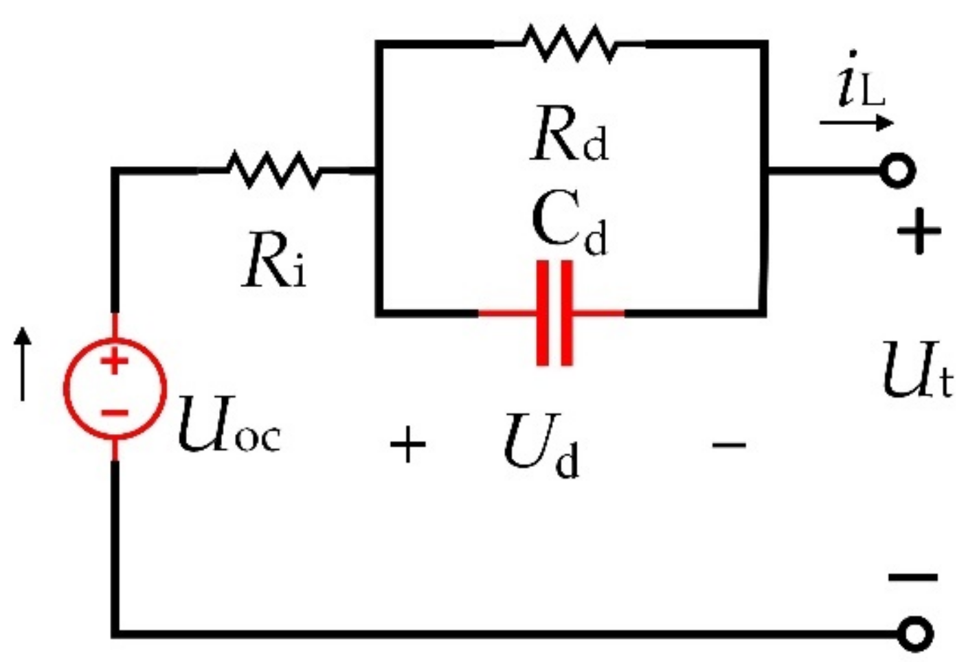
The establishment of ultracapacitor model plays a significant role in SOC estimation, and it is necessary to select a suitable model. The equivalent circuit model is usually selected for ultracapacitor modeling for its simpler structure and lower computational burden. The conventional models include Rint model, Thevenin model, Dual Polarization model, Classical Equivalent Circuit model and Three-branch model et.al. In this paper, the Thevenin model is applied to describe ultracapacitor characteristics, which consists of a voltage source, an ohmic internal resistance as well as an RC parallel network. The schematic diagram of the Thevenin model is shown in Figure 1.

Figure 1.
The schematic diagram of the Thevenin model.
Based on the Kirchhoff’s laws, the state-space equation of the Thevenin model can be listed as Equation (1).
where represents the ohmic internal resistance; defines the polarization resistance, and the polarization capacitance is indicated as ; the polarization voltage of the parallel RC network can be denoted as ; the terminal voltage is , and the open circuit voltage means as . Furthermore, the discretizing process of Equation (1) can be described by Equation (2), where τ is the time constant.
2.2. Model Parameter Identification
In this paper, genetic algorithm (GA) is used to identify model parameters of ultracapacitor, which is derived from biological field. It is well known that the GA is equipped with characteristics of fast random search, high computation efficiency and simple process. Based on the experimental data of Hybrid Pulse Power Characteristic (HPPC) at different temperatures (−10 °C, 10 °C, 25 °C and 40 °C), the GA is utilized to identify , and τ for the Thevenin model.
The Maxwell ultracapacitor with 2.7V-1500F is chosen to conduct the characteristic experiment at −10 °C, 10 °C, 25 °C and 40 °C, respectively. The average of capacitance test is regarded as the rated capacitance of ultracapacitors. The calculated capacities for ultracapacitors at different temperatures are listed in Table 1. Moreover, the identification process of Thevenin model at different temperatures can be summarized in Table 2.

Table 1.
The rated ultracapacitor capacities at different temperatures.
Table 2.
The identification process of Thevenin model at different temperatures.
In order to obtain optimal parameters, the ranges of , and τ are set to [1 × 10⁻⁶, 1 × 10⁻³], [1 × 10⁻⁶, 1 × 10⁻³] and [0, 0.2] in the process of implementing GA, respectively. Subsequently, the parameter identification results of ultracapacitor for different SOC intervals and temperatures are obtained, which is shown in Table 3. From Table 3, in the low temperature environment, the change rates of ohmic internal resistance and polarization resistance of ultracapacitor gradually increase with the decrease of temperature, and the maximum change rates are 96.464% and 98.654%, respectively. Under the high temperature environment, the ohmic internal resistance and polarization resistance change rate of the ultracapacitor are correspondingly 95.285% and 96.071%. At room temperature, the change rate of time constant of ultracapacitor is the largest, which is 95.431%. It can be seen that the ambient temperature has a great influence on the ultracapacitor parameters. Therefore, it is very necessary to consider the temperature factor when establishing the ultracapacitor model.
Table 3.
Parameter identification results of ultracapacitor for different SOC intervals and temperatures.
2.3. Evaluation of Thevenin Model
As is known to all, the validation of model accuracy is critical in the SOC estimation. Therefore, the model is employed in UDDS conditions to analysis the terminal voltage errors. The simulation results are shown in Figure 2. The Maximum Error (ME), Mean Absolute Error (MAE) and Root Mean Square Error (RMSE) are applied to evaluate the model in this study. Moreover, the ME, MAE and RMSE can be correspondingly described as Equations (3)–(5). Due to the less application of data in the lower SOC intervals in practice, a linear interpolation method is utilized to acquire the model parameters at each moment under 0.1 and 1.0 SOC internals. The terminal voltage error statistical results at different temperatures are listed in Table 4.
where and indicates reference and prediction value, respectively; n presents the data length.
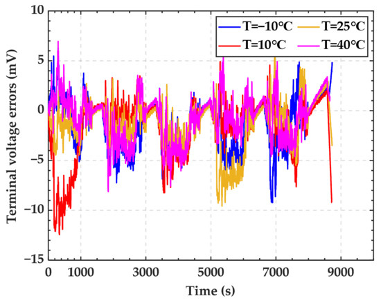
Figure 2.
The terminal voltage error results.
Table 4.
The terminal voltage error statistical results.
From the Figure 2, the Thevenin model at different temperatures has high accuracy, and the maximum ME is less than 13 mV. Taking 25 °C for example, the Table 4 shows that the ME, MAE and RMSE of the model are 9.563 mV, 1.912 mV and 2.718 mV, respectively. It turns out that the selected identification method has good performance in the ultracapacitor modeling. Compared with other temperatures, the model at 40 °C has the lowest errors, the ME, MAE and RMSE are correspondingly 8.131 mV, 1.782 mV and 2.319 mV. Moreover, the ME, MAE and RMSE at different temperatures are within 12.440 mV, 2.170 mV and 3.350 mV. The aforementioned analysis results demonstrate the model has the high accuracy at variable environment temperature.
2.4. Variable Temperature Modeling
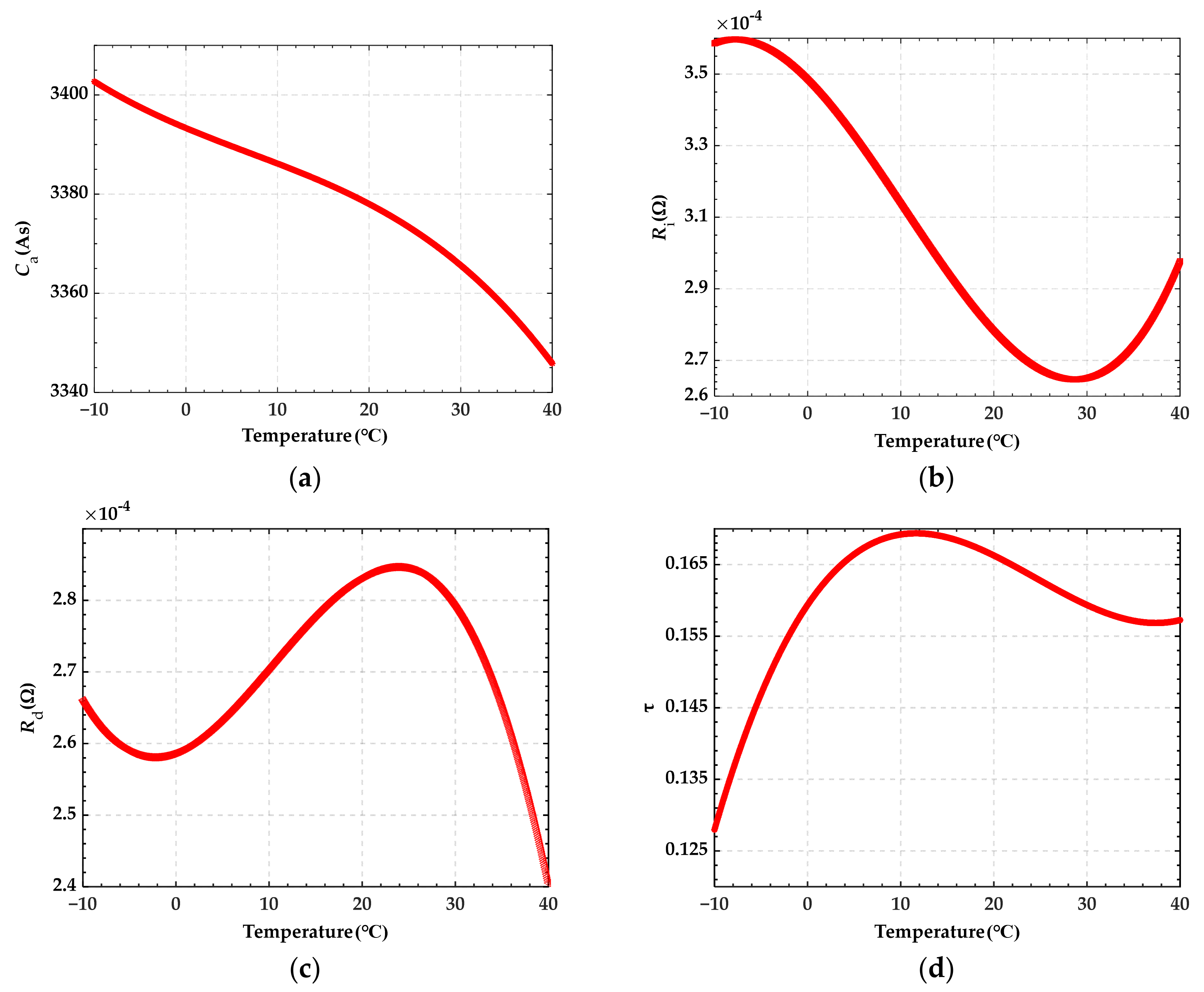
To analysis the mapping relationship between temperatures and Thevenin model parameters, a variable temperature model at −10 °C, 10 °C, 25 °C and 40 °C is established in this paper. In addition, the variable temperature model is subdivided into capacitance-T model, parameters-T model and open circuit voltage-T model. The modeling process is described below.
To obtain the ultracapacitor capacitances at different temperatures, a capacitance-T model is established based on the rated capacities. Furthermore, the mapping relationship between capacitance and temperature is acquired by polynomial fitting, as can be seen in Equation (6). Similarly, the parameters-T model can be described as Equations (7)–(9), respectively. Furthermore, the fitting results can be shown in Figure 3, respectively. As can be seen from Figure 3a, the capacitance gradually decreases with increasing temperature. The aforementioned models can be used to acquire accurate capacitance and parameters in multi-stress environments.

Figure 3.
The change of capacitance and parameters at different temperatures: (a) Capacitance-T fitting curve; (b) Ohmic internal resistance-T fitting curve; (c) Polarization resistance-T fitting curve; (d) Time constant-T fitting curve.
The open circuit voltage is obtained by fitting the selected SOC points with high stability, and the temperature will affect the battery SOC, which in turn will affect the open circuit voltage. Therefore, during the establishment of the open circuit voltage-T model, the influence of temperature and SOC factors are considered. Moreover, a polynomial fit of temperature, SOC and the open-circuit voltage is implemented, and the functional relationship is listed in Equation (10). The fitting result is shown in Figure 4.
where z denotes SOC and T indicates temperature. Based on the open circuit voltage-T model, the value of can be obtained under arbitrary SOC interval and temperature. Furthermore, the model can accurately describe the mapping relationship among open-circuit voltage, temperature and SOC.
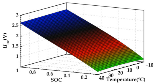
Figure 4.
The change of open circuit voltage under different SOC and temperatures.
In summary, the variable temperature model is established by polynomial fitting the model parameters and temperature, which is a function of temperature. It can be described as Equation (11). In the other words, the model parameters of the variable temperature model can be obtained at a certain temperature according to Equation (11). The efficiency of model parameter acquisition at different temperatures can be promoted for the establishment of variable temperature model.
3. Ultracapacitor SOC Estimation Methods
3.1. State of Charge Definition
SOC defines a present available capacitance of ultracapacitor, which can be calculated as Equation (12).
where is the initial SOC; indicates the estimated SOC; the coulomb efficiency can be denoted as . To improve computational efficiency, is set to 1 in this paper. In addition, represents the maximum available capacitance of ultracapacitor. The defined SOC is regarded as the referred SOC in this paper, which is employed to compare with the accuracy of other SOC estimation methods.
3.2. Adaptive Extended Kalman Filter (AEKF) Algorithm
The noise matrix of the extended Kalman filter is often preset, and the selection of the matrix often affects the prediction accuracy of the filter. In this paper, the AEKF with adaptive update feature is selected to improve the prediction accuracy. Meanwhile, the shortcoming that the preset noise matrix is difficult to adapt to the dynamic characteristics of ultracapacitors can be tackled. Based on the extended Kalman filter, an adaptive noise covariance matching process is carried out to realize the adaptive real-time update of the system noise and the observed noise covariance. Furthermore, the negative effect of noise on the estimation accuracy is weakened. The arbitrary nonlinear discrete system can be described by two functions, which are known as system state equation function and system observation function . In addition, the system state-space equation is denoted as Equation (13).
where X represents the system state variables, and it contains SOC and polarization resistance in this paper; u indicates the system input current; the system output estimation can be denoted as y; w expresses the system noise whose covariance is Q; v represents the observed noise and its covariance is R. The mean values of w and v are both zero, but they are independent.
The iteration processes of AEKF are as follows:
Step1: Initialize the filtering parameters. Determine the initial values of the state variable X, the error covariance P, the system noise covariance Q, and the system observation noise covariance R.
Step2: Predict the system state and covariance, as shown in Equation (14). The current moment estimate is obtained from the previous moment value.
Step3: Calculate the Kalman filter gain, which is shown in Equation (15). The gain is mainly used for the modification of state variables and error covariance.
Step4: Compute the innovation matrix, which is listed in Equation (16). This matrix is also applied to update the state variables and the noise covariance.
Step5: Adaptively update the noise covariance, which can be described as Equation (17).
Step6: Update the system state variable and covariance, as shown in Equation (18). The gain and innovation matrix are used to update the state variables and error covariance.
where and are state variables, which represent the optimal state estimate and priori estimate, respectively. The posteriori error covariance matrix and priori error covariance matrix are denoted as and , respectively; Q and R are noise covariance matrices, where Q denotes the system noise covariance and R indicates the observed noise covariance; the observation matrix can be defined as H; e represents the terminal voltage error; the adaptive noise covariance matching quantity can be denoted as D; and I is an unit matrix.
3.3. NARX-AEKF Fusion SOC Estimation
Nonlinear Auto-Regressive Model with Exogenous Inputs (NARX) is conventionally applied to prediction for time series data. The reason is that the feedback and delay layer are considered in the network training part to realize a dynamic recursive process [38]. Additionally, the method can predict the next time state target value by iterating over the past state. Hence, in order to take full advantage of NARX superiority, the combination of NARX and AEKF is proposed to realize ultracapacitor SOC estimation.
The key to the fusion method is to train the neural network by adopting the AEKF off-line data. To improve the SOC prediction accuracy, the output of the neural network is applied to compensate the AEKF estimation. The operation steps of this fusion method are listed as follows.
Step 1: Iterate the AEKF. The off-line data is iterated by using AEKF, and thereby the terminal voltage observation error e, Kalman gain K, and the residual error between state prediction and AEKF optimal estimate is obtained. The above obtained data constitutes the sample library.
Step 2: Train neural network. The e, K and are selected as inputs of neural network. The difference between the referred SOC and the AEKF-estimated SOC is employed as the output of neural network. Afterwards, the 80 percentage of the sample library is chosen as the training sample. In order to verify the network accuracy, the remaining data is utilized as the testing sample.
Step 3: SOC fusion estimation. The fused SOC is the addition between the network output and the AEKF-estimated SOC, as shown in Equation (19). The implementation flowchart of the SOC fusion estimation method is indicated in Figure 5.
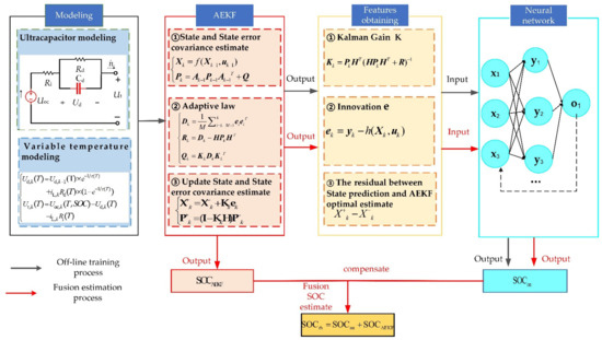
Figure 5.
An implementation flowchart of the SOC fusion estimation method.
4. Evaluations
4.1. Evaluation of Variable Temperature Model
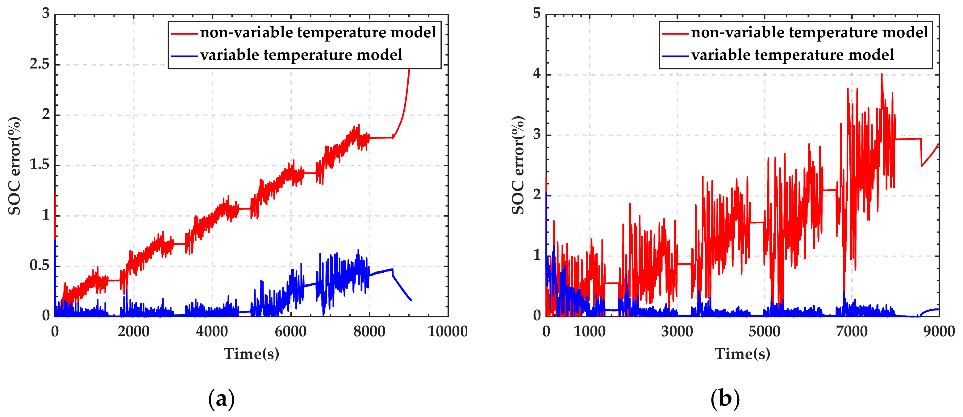
In order to verify the performance of the variable temperature model, a systematic comparison between the NARX-AEKF SOC fusion method with variable and non-variable temperature model is conducted at −10 °C and 40 °C. In addition, the SOC fusion estimation results and estimation errors with variable and non-variable temperature model at −10 °C and 40 °C are correspondingly shown in Figure 6 and Figure 7. The Maximum Error (ME), Mean Absolute Error (MAE) and Root Mean Square Error (RMSE) are applied to evaluate the proposed method in this study.
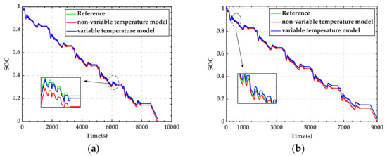
Figure 6.
The SOC fusion estimation results with variable and non-variable temperature model at −10 °C and 40 °C: (a) SOC estimation results at −10 °C; (b) SOC estimation results at 40 °C.

Figure 7.
The SOC estimation errors with variable and non-variable temperature model at −10 °C and 40 °C: (a) SOC estimation errors at −10 °C; (b) SOC estimation errors at 40 °C.
The SOC error statistical results of two models between estimated and referred values at −10 °C and 40 °C are listed in Table 5. Compared with the non-variable temperature model, the ME, MAE and RMSE of SOC estimation with variable temperature model at −10 °C are correspondingly reduced by 71.012%, 86.070% and 81.425%. Similarly, the reduction of ME, MAE and RMSE of SOC estimation at 40 °C are 49.003%, 93.654% and 90.187%, respectively. Based on the error statistical results, the proposed variable temperature model has higher accuracy and applicability than that of non-variable.
Table 5.
The SOC error statistical results of two models between estimated and referred values at −10 °C and 40 °C.
4.2. Evaluation of SOC Fusion Estimation Method
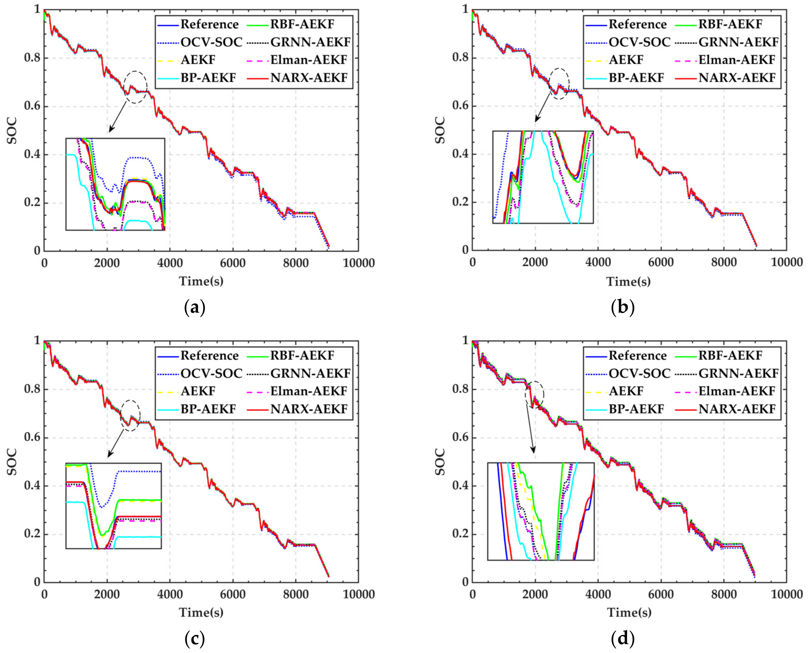
In order to evaluate the accuracy of NARX-AEKF, the classical BP neural network, radial basis neural network (RBF), generalized regression neural network (GRNN) and Elman neural network are combined with AEKF to estimate ultracapacitor SOC, respectively. Subsequently, the comparison of SOC estimation results, including the AEKF-based method, five SOC fusion estimation methods, OCV-SOC method and Ampere-hour method is conducted on UDDS conditions. The SOC estimation results of eight methods at different temperatures (−10 °C, 10 °C, 25 °C, 40 °C) are shown in Figure 8. Moreover, the SOC estimation statistical errors for the seven methods at different temperatures are summarized in Table 6.
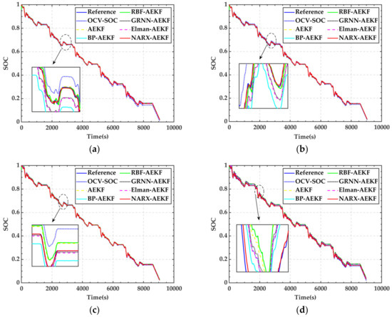
Figure 8.
The SOC estimation results of seven methods at different temperatures: (a) SOC estimation results at −10 °C; (b) SOC estimation results at 10 °C; (c) SOC estimation results at 25 °C; (d) SOC estimation results at 40 °C.
Table 6.
The SOC estimation statistical errors for the seven methods at different temperatures.
From Table 6, the proposed SOC fusion estimation method, combined with the neural network and AEKF, has high accuracy at different temperatures. The ME, MAE and RMSE of the method mentioned are less than 5.000%, 1.310% and 1.350%, respectively. Moreover, the proposed SOC fusion estimation methods with variable temperature model have excellent applicability, and their RMSEs at −10 °C, 10 °C, 25 °C and 40 °C are 0.175%, 0.185%, 0.270%, 0.915%, respectively. Compared with the RBF-AEKF, the MEs of NARX-AEKF at 10 °C, 25 °C and 40 °C are correspondingly decreased by 80.025%, 77.498% and 28.660%, and the MAEs are reduced by 94.397%, 91.338% and 92.855%, respectively. This is mainly attributed to the superiority of NARX neural networks to other neural networks in terms of structure and function. It can obtain better mapping relationship between model parameters and ultracapacitor SOC, which is beneficial to improve its estimation accuracy. For example, the ME, MAE and RMSE of the proposed NARX-AEKF at 25 °C are 0.816%, 0.031% and 0.047%, respectively. While the AEKF are correspondingly 1.553%, 0.368% and 0.448%, which illustrates that the NARX neural network has the prominent compensation characteristic. Furthermore, compared with the OCV-SOC method, the ME and RMSE of NARX-AEKF are correspondingly reduced by 66.764% and 55.494% at least. Moreover, the MEs of the proposed method at −10 °C, 10 °C and 25 °C are less than 1%, while that of OCV-SOC at different temperatures are greater than 1%. It turns out that the proposed method has more excellent performance than OCV-SOC method at variable temperature environment. However, the accuracy of neural network trained by experimental data in low temperature environment suffers from instability. For instance, compared with AEKF, the ME, MAE and RMSE of NARX-AEKF increase by 37.746%, 30.135% and 63.649% at −10 °C, respectively. To sum up, the proposed NARX-AEKF has better adaptability than the classical Ampere-hour method, the well-established OCV-SOC method and the above mentioned methods with its higher estimation accuracy and stronger robustness even in variable temperature environment.
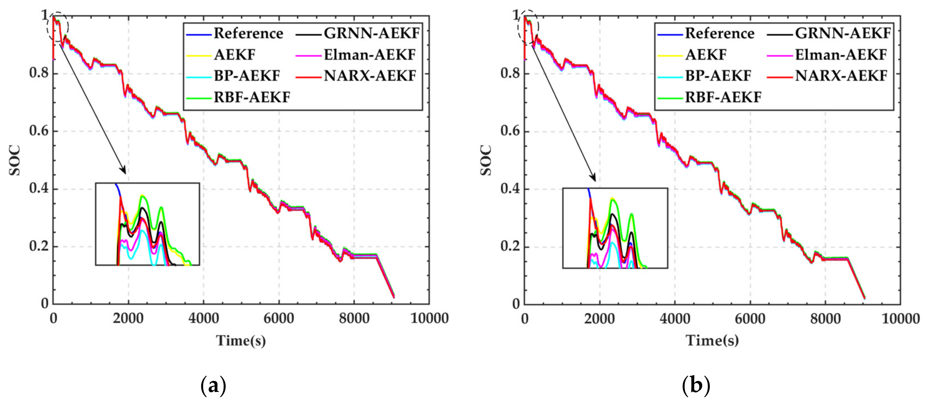
In practical applications, the initial SOC error of ultracapacitors usually affects the estimation accuracy of the observer. Therefore, the estimation accuracy of the NARX-AEKF estimation method is verified when the initial error of SOC is 0.150 in this paper. The estimation results of different SOC fusion estimation methods are shown in Figure 9. The simulation results illustrate that the proposed method achieves good estimation accuracy under different temperatures in the presence of initial SOC error. Furthermore, the error and convergence time statistics of different SOC estimation methods are listed in Table 7. Due to the initial error, the ME is obtained from the error data after 50 s.

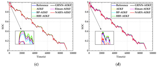
Figure 9.
The estimation results of different SOC fusion estimation methods: (a) SOC estimation results at −10 °C; (b) SOC estimation results at 10 °C; (c) SOC estimation results at 25 °C; (d) SOC estimation results at 40 °C.
Table 7.
The error and convergence time statistics of different SOC estimation methods.
From Table 7, in the presence of initial error, NARX-AEKF has the highest accuracy among all SOC fusion estimation methods at different temperatures (−10 °C, 10 °C, 25 °C and 40 °C). Compared with BP-AEKF, the ME, MAE and RMSE of the proposed method are decreased by 86.158%, 96.387% and 76.564% at most, respectively. This is because the NARX neural network considers the feedback process, which improves the estimation accuracy to a certain extent. Compared with AEKF, the proposed NARX-AEKF has the largest reduction of ME, MAE and RMSE at −10 °C, which are 235.912%, 99.159% and 122.154%, respectively. The NARX neural network compensates the AEKF estimation and reduces the gap between the estimated value and the reference value; thereby the estimation accuracy is greatly improved. Furthermore, the convergence time of the proposed SOC fusion estimation method is less than 5.000 s when the initial SOC error is set at 0.150. The above analysis results demonstrate that the proposed NARX-AEKF SOC fusion estimation method has good performance in SOC initial error and different temperature environments.
5. Conclusions
In this paper, an ultracapacitor SOC estimation method based on NARX neural network and AEKF in variable temperature environment is proposed. Firstly, Based on Thevenin model, the influence of temperature is considered, and a high-precision variable temperature model is established with the experimental data of ultracapacitor at different temperatures. Secondly, the SOC estimation results between NARX-AEKF with the non-variable and variable temperature model are compared and analyzed. Moreover, the results illustrate that the SOC fusion estimation method with variable temperature model has higher accuracy. The ME, MAE and RMSE are decreased by 71.012%, 93.654% and 90.187%, respectively., Thirdly, the estimation results of different SOC fusion estimation methods at different temperatures without initial error and when the initial error is 0.150 are compared.
Finally, the results show that the accuracy of NARX-AEKF fusion method is lower than other estimation methods without considering the initial error of SOC at −10 °C, but the ME, MAE and RMSE are reduced by 82.708%, 92.855% and 89.547% at the other three temperatures, respectively. The SOC estimation accuracy of NARX-AEKF with initial SOC error is the highest at all temperatures (−10 °C, 10 °C, 25 °C and 40 °C), and the ME, MAE and RMSE are 1.145%, 0.087% and 0.221%. The proposed method utilizes NARX neural network to compensate the AEKF estimation. In turn, the influence of noise is reduced, and the SOC estimation accuracy is effectively enhanced. At the same time, the accuracy and applicability of the NARX-AEKF in wide temperature environment is improved for the application of variable temperature model.
Author Contributions
Conceptualization, C.W. and A.T.; methodology, C.F.; software, C.F.; validation, C.F.; formal analysis, C.F.; investigation, C.W. and C.F.; resources, C.W., A.T. and B.H.; data curation, C.W. and C.F.; writing—original draft preparation, C.F.; writing—review and editing, C.W., A.T., B.H. and Z.Z.; visualization, C.F.; supervision, C.W.; project administration, C.W.; funding acquisition, C.W., B.H., A.T. and Z.Z. All authors have read and agreed to the published version of the manuscript.
Funding
This research was funded by the National Natural Science Foundation of China (Grant No. 51907136), Zigong Key Science and Technology Project (Grant No. 2019YYJC14), Talent Introduction Project of Sichuan University of Science and Engineering (Grant No. 2019RC15), Chongqing Universities Innovation Research Group Project (Grant No. CXQT21027), Natural Science Foundation of Chongqing, China (Grant No.cstc2021jcyj-msxmX0464), Scientific Research Foundation of Chongqing University of Technology (Grant No. 2021ZDZ004) and Foundation of Artificial Intelligence Key Laboratory of Sichuan Province (Grant No. 2020RYY01). The systemic experiments were performed at the Advanced Energy Storage and Application (AESA) Group, Beijing Institute of Technology.
Institutional Review Board Statement
Not applicable.
Informed Consent Statement
Not applicable.
Data Availability Statement
Not applicable.
Conflicts of Interest
The authors declare no conflict of interest.
References
- Župan, I.; Šunde, V.; Ban, Ž.; Krušelj, D. Algorithm with temperature-dependent maximum charging current of a supercapacitor module in a tram regenerative braking system. J. Energy Storage 2021, 36, 102378. [Google Scholar] [CrossRef]
- Ahmad, F.; Khalid, M.; Panigrahi, B.K. Development in energy storage system for electric transportation: A comprehensive review. J. Energy Storage 2021, 43, 103153. [Google Scholar] [CrossRef]
- Zhang, X.; Pei, W.; Mei, C.X.; Deng, W.; Tan, J.X.; Zhang, Q.Q. Transform from gasoline stations to electric-hydrogen hybrid refueling stations: An islanding DC microgrid with electric-hydrogen hybrid energy storage system and its control strategy. Int. J. Electr. Power Energy Syst. 2022, 136, 107684. [Google Scholar] [CrossRef]
- Wang, X.; Luo, Y.B.; Qin, B.; Peng, J.M.; Zhou, Y.; Sun, Z.C. Ultracapacitor Energy Storage Systems based on Dynamic Setting and Coordinated Control for Urban Trains. IFAC-Papers OnLine 2020, 53, 14954–14959. [Google Scholar] [CrossRef]
- Shi, X.Y.; Zheng, S.H.; Wu, Z.S.; Bao, X.H. Recent advances of graphene-based materials for high-performance and new-concept supercapacitors. J. Energy Chem. 2018, 27, 25–42. [Google Scholar] [CrossRef] [Green Version]
- Lei, X.; Zhao, X.; Wang, G.P.; Liu, W.Y. A Novel Temperature–Hysteresis Model for Power Battery of Electric Vehicles with an Adaptive Joint Estimator on State of Charge and Power. Energies 2019, 12, 3621. [Google Scholar] [CrossRef] [Green Version]
- Chin, C.S.; Gao, Z.H. State-of-Charge Estimation of Battery Pack under Varying Ambient Temperature Using an Adaptive Sequential Extreme Learning Machine. Energies 2018, 11, 711. [Google Scholar] [CrossRef] [Green Version]
- Xiong, R.; Gong, X.Z.; Mi, C.C.; Sun, F.C. A Robust State-of-Charge Estimator for Multiple Types of Lithium-ion Batteries Using Adaptive Extended Kalman Filter. J. Power Sources 2013, 243, 805–816. [Google Scholar] [CrossRef]
- Mohammadi, F. Lithium-ion battery State-of-Charge estimation based on an improved Coulomb-Counting algorithm and uncertainty evaluation. J. Energy Storage 2022, 48, 104061. [Google Scholar] [CrossRef]
- Singh, K.V.; Bansal, H.O.; Singh, D. Hardware-in-the-loop implementation of ANFIS based adaptive SoC estimation of lithium-ion battery for hybrid vehicle applications. J. Energy Storage 2020, 27, 101124. [Google Scholar] [CrossRef]
- Zheng, Y.J.; Cui, Y.F.; Han, X.B.; Dai, H.F.; Ouyang, M.G. Lithium-ion battery capacity estimation based on open circuit voltage identification using the iteratively reweighted least squares at different aging levels. J. Energy Storage 2021, 44, 103487. [Google Scholar] [CrossRef]
- Dang, X.J.; Yan, L.; Jiang, H.; Wu, X.R.; Sun, H.X. Open-circuit voltage-based state of charge estimation of lithium-ion power battery by combining controlled auto-regressive and moving average modeling with feedforward-feedback compensation method. Int. J. Electr. Power Energy Syst. 2017, 90, 27–36. [Google Scholar] [CrossRef]
- Chen, X.K.; Lei, H.; Xiong, R.; Shen, W.X.; Yang, R.X. A novel approach to reconstruct open circuit voltage for state of charge estimation of lithium ion batteries in electric vehicles. Appl. Energy 2019, 255, 113758. [Google Scholar] [CrossRef]
- Zhang, L.; Hu, X.S.; Su, S.; Dorrell, D.G. Robust State-of-Charge Estimation of Ultracapacitors for Electric Vehicles. In Proceedings of the 13th IEEE International Conference on Industrial Informatics (INDIN), Cambridge, UK, 22–24 July 2015; pp. 1296–1301. [Google Scholar]
- Guo, Y.F.; Zhao, Z.S.; Huang, L.M. SoC estimation of Lithium battery based on improved BP neural network. Energy Procedia 2017, 105, 4153–4158. [Google Scholar] [CrossRef]
- Fasahat, M.; Manthouri, M. State of charge estimation of lithium-ion batteries using hybrid autoencoder and Long Short Term Memory neural networks. J. Power Sources 2020, 469, 228375. [Google Scholar] [CrossRef]
- Wang, Q.; Ye, M.; Wei, M.; Lian, G.Q.; Wu, C.G. Co-estimation of state of charge and capacity for lithium-ion battery based on recurrent neural network and support vector machine. Energy Rep. 2021, 7, 7323–7332. [Google Scholar] [CrossRef]
- Xi, Z.M.; Wang, R.; Fu, Y.H.; Mi, C. Accurate and reliable state of charge estimation of lithium-ion batteries using time-delayed recurrent neural networks through the identification of overexcited neurons. Appl. Energy 2022, 305, 117962. [Google Scholar] [CrossRef]
- Zhang, G.Y.; Xia, B.Z.; Wang, J.M.; Ye, B.; Chen, Y.C.; Yu, Z.J.; Li, Y.H. Intelligent state of charge estimation of battery pack based on particle swarm optimization algorithm improved radical basis function neural network. J. Energy Storage 2022, 50, 104211. [Google Scholar] [CrossRef]
- Weigert, T.; Tian, Q.; Lian, K. State-of-charge prediction of batteries and battery–ultracapacitor hybrids using artificial neural networks. J. Power Sources 2010, 196, 4061–4066. [Google Scholar] [CrossRef]
- Yang, C.F.; Wang, X.Y.; Fang, Q.H.; Dai, H.F.; Cao, Y.Q.; Wei, X.Z. An online SOC and capacity estimation method for aged lithium-ion battery pack considering cell inconsistency. J. Energy Storage 2020, 29, 101250. [Google Scholar] [CrossRef]
- Wei, Z.B.; Xiong, R.; Lim, T.M.; Meng, S.J.; Skyllas-Kazacos, M. Online monitoring of state of charge and capacity loss for vanadium redox flow battery based on autoregressive exogenous modeling. J. Power Sources 2018, 402, 252–262. [Google Scholar] [CrossRef]
- Saha, P.; Dey, S.; Khanra, M. Accurate estimation of state-of-charge of ultracapacitor under uncertain leakage and open circuit voltage map. J. Power Sources 2019, 434, 226696. [Google Scholar] [CrossRef]
- Wang, J.; Xiong, R.; Li, L.L.; Fang, Y. A comparative analysis and validation for double-filters-based state of charge estimators using battery-in-the-loop approach. Appl. Energy 2018, 229, 648–659. [Google Scholar] [CrossRef]
- Snoussi, J.; Elghali, S.-B.; Zerrougui, M.; Bensoam, M.; Benbouzid, M.; Mimouni, M.F. Unknown input observer design for lithium-ion batteries SOC estimation based on a differential-algebraic model. J. Energy Storage 2020, 32, 101973. [Google Scholar] [CrossRef]
- Liu, C.; Wang, Y.J.; Chen, Z.H.; Ling, Q. A variable capacitance based modeling and power capability predicting method for ultracapacitor. J. Power Sources 2018, 374, 121–133. [Google Scholar] [CrossRef]
- Nadeau, A.; Hassanalieragh, M.; Sharma, G.; Soyata, T. Energy awareness for ultracapacitors using Kalman filter state-of-charge tracking. J. Power Sources 2015, 296, 383–391. [Google Scholar] [CrossRef] [Green Version]
- Jarraya, I.; Masmoudi, F.; Chabchoub, M.H.; Trabelsi, H. An online state of charge estimation for Lithium-ion and ultracapacitor in hybrid electric drive vehicle. J. Energy Storage 2019, 26, 100946. [Google Scholar] [CrossRef]
- Zhang, L.; Hu, X.S.; Wang, Z.P.; Sun, F.C.; Dorrell, D.G. Fractional-Order Modeling and State-of-Charge Estimation for Ultracapacitors. J. Power Sources 2016, 314, 28–34. [Google Scholar] [CrossRef]
- Tian, J.P.; Xiong, R.; Shen, W.X.; Lu, J.H. State-of-charge estimation of LiFePO4 batteries in electric vehicles: A deep-learning enabled approach. Appl. Energy 2021, 291, 116812. [Google Scholar] [CrossRef]
- Zhang, R.F.; Xia, B.Z.; Li, B.H.; Cao, L.B.; Lai, Y.Z.; Zheng, W.W.; Wang, H.W.; Wang, W.; Wang, M.W. A Study on the Open Circuit Voltage and State of Charge Characterization of High Capacity Lithium-Ion Battery Under Different Temperature. Energies 2018, 11, 2408. [Google Scholar] [CrossRef] [Green Version]
- Chiang, C.J.; Yang, J.L.; Cheng, W.C. Temperature and state-of-charge estimation in ultracapacitors based on extended Kalman filter. J. Power Sources 2013, 234, 234–243. [Google Scholar] [CrossRef]
- Khaleghi, S.; Karimi, D.; Beheshti, S.H.; Hosen, M.S.; Behi, H.; Berecibar, M.; Van Mierlo, J. Online health diagnosis of lithium-ion batteries based on nonlinear autoregressive neural network. Appl. Energy 2021, 282, 116159. [Google Scholar] [CrossRef]
- Kleiner, J.; Stuckenberger, M.; Komsiyska, L.; Endisch, C. Real-time core temperature prediction of prismatic automotive lithium-ion battery cells based on artificial neural networks. J. Energy Storage 2021, 39, 102588. [Google Scholar] [CrossRef]
- Peng, N.; Zhang, S.Z.; Zhang, X.W. Co-estimation for capacity and state of charge for lithium-ion batteries using improved adaptive extended Kalman filter. J. Energy Storage 2021, 40, 102559. [Google Scholar]
- Shi, N.; Chen, Z.W.; Niu, M.; He, Z.J.; Wang, Y.R.; Cui, J. State-of-charge estimation for the lithium-ion battery based on adaptive extended Kalman filter using improved parameter identification. J. Energy Storage 2022, 45, 103518. [Google Scholar] [CrossRef]
- Zhang, Z.Y.; Jiang, L.; Zhang, L.Z.; Huang, C.X. State-of-charge estimation of lithium-ion battery pack by using an adaptive extended Kalman filter for electric vehicles. J. Energy Storage 2021, 37, 102457. [Google Scholar] [CrossRef]
- Hasan, M.M.; Pourmousavi, S.A.; Ardakani, A.J.; Saha, T.K. A data-driven approach to estimate battery cell temperature using a nonlinear autoregressive exogenous neural network model. J. Energy Storage 2020, 32, 101879. [Google Scholar] [CrossRef]


Publisher’s Note: MDPI stays neutral with regard to jurisdictional claims in published maps and institutional affiliations. |
© 2022 by the authors. Licensee MDPI, Basel, Switzerland. This article is an open access article distributed under the terms and conditions of the Creative Commons Attribution (CC BY) license (https://creativecommons.org/licenses/by/4.0/).