Abstract
The development of primary frequency regulation (FR) technology has prompted wind power to provide support for active power control systems, and it is critical to accurately assess and predict the wind power FR potential. Therefore, a prediction model for wind power virtual inertia and primary FR potential is proposed. Firstly, the primary FR control mode is divided and the mapping relationship of operating wind speed and FR potential is constructed. Secondly, a hybrid prediction method of singular spectrum analysis (SSA) and Gaussian process regression (GPR) is proposed for predicting the speed of wind. Finally, the wind speed sequence is adopted to calculate the FR potential with various regulation modes in future time. The results show the advantages of the proposed method in the prediction accuracy of wind power FR potential and the ability to characterize the uncertainty information of the prediction results. Accurate modeling and prediction of wind power FR potential can significantly promote wind turbines to implement fine control of primary FR and optimal allocation of FR capacity within wind farm and group. Based on the actual operation data, the deterministic prediction and probability prediction of the FR potential of wind farms are conducted in this paper.
1. Introduction
According to the World Wind Energy Association, in 2020, the global annual installed capacity of wind energy and total capacity reached 93 GW and 743 GW, respectively, and a year-on-year increase of 53% and 14.3% [1] over the end of 2019. With the increasing penetration of wind power, the traditional synchronous generating units are replaced by wind power in large numbers, which decreases the rotational inertia and frequency stability of power systems, and increases the requirement of frequency regulation (FR) [2]. The large-scale access of wind power without inertia and frequency active support capability brings a great challenge [3] to the reliability of the power system. Frequency control technology of a converter makes it possible for wind turbines to participate in grid frequency regulation through quickly releasing FR potential contained in the turbine at the moment of system disturbance [4]. Thus, the effective prediction of FR potential is of great significance to the dispatching department for power generation planning, reasonable arrangement of rotating reserve, and improvement of renewable power penetration rate.
The technologies of wind generation participating in FR mainly include virtual inertia control, over-speed standby control, pitch control, and cooperative control [5,6,7]. To accurately quantify the impact of wind power participation in power system FR, there is an urgent need to quantitatively analyze the frequency regulation potential of wind turbines. Ref. [8] analyzed the equivalent time constant of the wind power frequency response, which offers a theoretical basis for studying the characteristics of power systems with high proportion of renewable power. Ref. [9] proposed an assessment model of the primary frequency standby power to analyze the wind power deloading operation under different scenarios. Refs. [10,11] estimated the magnitude of kinetic energy release from wind farms and its effect on dynamic frequency improvement. Ref. [12] analyzed the contribution of wind power primary frequency regulation in the planning stage. Ref. [13] proposed a predictive control strategy based on a generalized predictive controller and applied it to the grid-side converter of wind turbines, so that it has the frequency support ability. Ref. [14] presents an analytical method to evaluate the wind turbine frequency support during the inertia response stage. However, there still remain some problems to be solved: the objects of current research include the effective benefits of wind power FR in specific scenarios, while the volatility and uncertainty of wind speed are not considered. Current research is usually based on the system level, while with the massive integration of wind power, the actual power grid becomes more complex and variable, and there is an urgent need to study the wind power FR potential in the site level. The equivalent modeling method for a single wind turbine is considered, and there is no specific method to quantify the FR potential of wind farms.
To address above problems, this paper analyzes in detail the dominant factors of wind power participation in system frequency regulation, proposes a quantitative analysis method for wind power FR potential, integrates the processing advantages of SSA [15], and GPR [16], a hybrid prediction method that comprehensively utilizes both technologies, is designed to achieve accurate and real-time prediction of the FR potential of wind farm [8].
2. Foundation of Wind Power Participation in FR
2.1. Virtual Inertial Response Principle
The FR power reflecting to frequency variation is introduced into the active power regulation of converters; thus, the inertia response and frequency response characteristics of the conventional generator are simulated by using the virtual inertia control. The wind power generation operates in maximum power point tracking (MPPT) mode under normal conditions. When the system frequency deviates from the reference power, the corresponding FR auxiliary power can be calculated by introducing the system frequency deviation and the frequency variation rate / [8].
where / represent the proportional/differential coefficients of system frequency deviation.
Reference value for the external loop control of the converter active power is
where represents the active reference power during MPPT operation.
Virtual inertia control enables wind turbines to quickly adjust electromagnetic power during system frequency abrupt variation by improved active control links, which plays a short-term frequency support role. Similar to conventional generators, wind turbines also store some rotor kinetic energy, when the frequency of wind turbine system changes, the response can be carried out by releasing the rotor kinetic energy. However, the stored kinetic energy of wind turbines is limited, which cannot solve the problem of frequency decline caused by large disturbances, and the transitional release of rotor kinetic energy also triggers low-speed protection causing a secondary system frequency drop. Therefore, the wind turbine should have a certain amount of active reserve, so that the wind power generation has the corresponding primary FR capability to improve the reliability of grid-connected operation.
2.2. Primary Frequency Regulation Principle
Wind turbine primary frequency regulation is divided into over-speed standby control and pitch control. Over-speed control is to realize the deloading operation of wind turbines through forcing the rotor speed exceeding the maximum power point tracking speed and storing active backup. Pitch control can change the output of wind generation through regulating the angle of wind blade, thus supporting the power systems’ frequency in case of failure [8].
The wind power characteristic curves of different speed are shown in Figure 1, in which the curves represent the relationship between wind power output and rotor speed at fixed wind speeds. When the wind turbine is in normal operation, the operating point A is the MPPT point corresponding to the current wind speed, and the operating point B is the over-speed point, the operating speed deviates from the MPPT point to realize the load reduction operation of the unit; the sub-optimal power operating point C is the variable pitch control load reduction point, that is, on the basis of the MPPT operating point pitch angle increases from β4 to β3 while keeping the rotational speed unchanged, and the corresponding wind power utilization coefficient is reduced due to the increase of the pitch angle. As the pitch angle increases, the corresponding energy utilization coefficient declines, and thus output power also decreases.
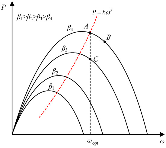
Figure 1.
Wind power primary frequency regulation principle.
The above two primary frequency regulation methods of wind turbines are realized by active standby. The differences between them are: the over-speed deloading control depends on the current and maximum wind speed of the wind turbine, and its application scope is limited, but the response speed is fast with converter control only. Over-speed standby control for deloading operation increases the rotate speed of wind turbines’ operation and kinetic energy stored in rotors at the same time, and enhances the inertial response and primary frequency regulation capability of wind turbines. Pitch control is usually adopted in medium/high wind speed scenarios. Given the uncertain wind speed of wind turbines’ operation, frequent pitch control will accelerate the wear of mechanical structure and slow response speed, but the adjustable range of pitch control is not limited.
2.3. Over-Speed Standby and Pitch Cooperative Control Area Division
The primary frequency regulation methods, over-speed standby, and pitch have different response speeds and can promote the improvement of transient as well as steady-state frequency characteristics of the power grid, respectively. Aimed at fully exploring the frequency regulation potential of different primary frequency regulation methods of wind turbines, and responding to system frequency deviation quickly, it is urgent to delineate the over-speed standby as well as pitch cooperative control area.
The characteristic curves regarding variable speed wind turbine rotor speed ω and output changing with wind speeds are demonstrated in Figure 2. When , insufficient wind speeds make frequency regulation of wind turbines impossible; when , wind turbines are in the MPPT region and are frequency regulated once by the over-speed standby control; when , the wind speed is high and the wind turbine is frequency regulated once by the pitch control. and are the minimum wind speed and rated wind speed involved in frequency regulation, respectively.
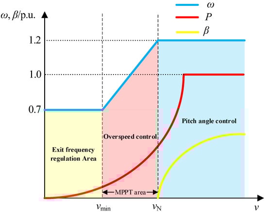
Figure 2.
The range of wind power primary frequency control.
To determine the active reserve required for primary frequency regulation, define the wind turbine deloading level as , then the active power output of the unit is (1 − ) after deloading. Combining the advantages of over-speed standby as well as pitch control, for a given deloading level, the over-speed standby is preferentially used for deloading, and the pitch control is used for deloading as soon as the over-speed reaches its upper limit.
The variable speed wind turbine model can be shown as:
where represents mechanical power of wind turbines; represents the air density; represents the swept area of wind wheels; represents the wind speed; represents the wind energy utilization coefficient; represents the pitch angle of wind turbines; represents the blade tip speed ratio, [8].
For a fixed wind speed, the power obtained by turbines depends on the wind energy utilization factor , i.e., on the values related to and . Varying the wind energy utilization coefficient leads to maximum power tracking under reduced load operation.
For a given deloading level of , there exists a unique critical wind speed . If , the reserved power deloading level can be achieved only by over-speed standby control, so it corresponds to = 0. If , the expected deloading level must be achieved by over-speed standby and variable pitch control. The critical wind speed calculation method is as follows:
where represents the wind energy utilization coefficient of turbines after deloading, represents the wind energy utilization coefficient at wind turbines’ maximum power tracking, represents the unique critical wind speed under the reserved deloading level , represents the unique speed of regarding the optimal blade tip speed ratio, and represents the maximum speed of wind turbines’ wheel.
The above equation can calculate the unique critical wind speed under each reserved load reduction level and fit to get the relationship curve between reserved load reduction level and critical wind speed. When , the wind turbine adopts over-speed deloading control to obtain the reserved deloading level, and the region is defined as region 1; when , the wind turbine adopts over-speed deloading control as well as pitch angle control together to obtain the reserved deloading level, and the region is defined as region 2; when , the wind turbine uses pitch angle control to obtain the reserved deloading level, and the region is considered to be region 3, and the FR region is calculated once. The division is shown in Figure 3.
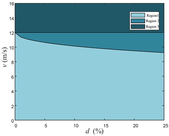
Figure 3.
Division of wind power primary FR cooperative control area.
3. Modeling the FR Potential of Wind Power Participation Systems
3.1. Analysis of Wind Power FR Influence Factors
Neglecting the system losses, the frequency response equation with wind power can be expressed as:
where and are the power system and wind power inertia time constants, respectively; is the system damping factor; is the system surge load, is the conventional thermal power unit frequency regulation power; represents the governor time constant; represents the unit regulation power; and are the respective wind turbine over-speed standby and pitch standby power.
The proportional coefficient and the differential coefficient determine the wind turbine generators to produce similar rotational inertia and damping characteristics as conventional generators. For different system perturbations and wind turbine generator FR auxiliary controller parameters, the wind power frequency response is different. Therefore, virtual inertia control should be used as an indicator to assess its frequency regulation potential by its maximum releasable rotor kinetic energy.
3.2. Wind Power Can Release Maximum Rotor Kinetic Energy
Virtual inertia response and over-speed standby release or absorb rotor kinetic energy through adjusting the speed, while the current blade tip speed ratio along with change of real-time wind speeds decide the generator speed. The rotor kinetic energy change before and after the speed change of the generator set running the maximum power tracking state is:
where represents the rotor speed before participation in the FR and represents the lowest boundary of rotor speed. Based on the definition of the equivalent virtual inertia time constant of the system, as shown in Figure 4, when MPPT is running, the correlation of the wind turbine time constant and wind speed can be obtained, as well as the maximum kinetic energy of the rotor released through frequency regulation.
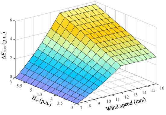
Figure 4.
Maximum rotor kinetic energy of the wind turbine.
The time constant of wind turbines belongs to an inherent parameter of the unit, and the larger its value, the greater the rotor kinetic energy is able to be released, while the secondary dip in frequency caused by the moment the unit exits the FR will be more obvious; the rotor speed is mapped according to the wind speed sequence and the kinetic energy of rotors because the MPPT strategy tracks the wind speed change in real time to maintain the optimal blade tip speed ratio.
3.3. Wind Power Backup Power
After the exit of wind turbines in FR, it begins to recover its speed and operates in MPPT mode. The kinetic energy released by rotors can be offset by stored kinetic energy during the participation of wind turbines in the FR process, and the speed, mechanical power, and electromagnetic power before and after the frequency regulation remain unchanged. The primary frequency control makes the wind turbine operate in the deloading mode. Since the response frequency change time scales of the two primary frequency regulation methods, over-speed control as well as pitch control, are different, the primary frequency control potential of wind farms is required to be quantified independently in the assessment. The over-speed control standby power can be expressed as:
Pitch control standby power is demonstrated as:
The wind turbine primary frequency regulation standby power under different boundary conditions is given in Figure 5. Over-speed standby only applies to scenarios with medium or high wind speeds. As shown in Figure 5, the pitch control has a larger range of standby power regulation.
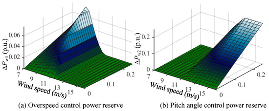
Figure 5.
Variable pitch standby power.
When wind turbines are restored to MPPT mode, compared to the initial phase of frequency regulation, additional unit standby power is generated. The unbalanced load in the original system is finally balanced by the FR power of thermal power units and the standby power of the wind power.
From Equation (5), we can get
Using the Laplace transform, suppose D = 0, we get
Moreover, from Equation (5), we can also get
The final expression is:
Therefore, the corresponding primary frequency regulation steady-state frequency deviation can be expressed using the final value theorem as:
where, and are the wind turbine over-speed standby and pitch standby power, respectively.
The above analysis shows that virtual inertia control of wind farms can offer transient frequency response, while backup power of primary frequency regulation can promote the improvement of the system steady-state frequency deviation. When wind turbines’ parameters are fixed, the change of wind speed can influence the rotor kinetic energy under MPPT mode [8]. With the reserved primary FR power, both the wind speed and the reserved load reduction level have an effect on the maximum released rotor kinetic energy and the reserved power.
4. Wind Power FR Potential Prediction Model
The analysis of the factors affecting the FR potential in Section 3.1 suggests that the wind power FR potential varies with the real-time wind speed, and the wind speed shows a chaotic, uncertain, and volatile sequence. To obtain the predicting accuracy of wind power FR potential, a hybrid prediction model framework dependent on SSA as well as GPR is proposed in this paper.
4.1. SSA
SSA is a sequence decomposition reconstruction method using singular value decomposition. It is generally divided into four steps [13]: embedding, singular value decomposition, diagonal averaging, and reconstruction. The specific process is as follows.
(1) Embedding. A one-dimensional time series z = [, , …, ] of length N can be transformed into a trace matrix based on the provided embedding dimension L.
where , , …, zi+L−1]T, i = 1, 2, …, K, and K = N − L + 1.
(2) Singular value decomposition performance on the trace matrix. The eigenvalues of the matrix XTX are found and arranged in a descending order based on the eigenvalue magnitude as corresponding to the eigenvalues. Let d be the number of non-zero eigenvalues, and define , then the singular value decomposition of the trace matrix X can be expressed as:
where ,, and Vi are the i-th values well as the respective left/right singular vectors of the trace matrix X.
(3) Diagonal averaging reduces the time series. x is an L×K matrix, and the elements is xij, such that L* = min(L,K), K* = max(L,K), n = L + K − 1, and satisfies x*ij = xij when L < Kij, otherwise x*ij = xji for the sub-matrix Xi reduced to obtain the sequence y1, y2, …, yN can be expressed as:
The performance of the decomposition algorithm depends a lot on the selection of embedding dimension L; a too small L will lead to modal under-decomposition affecting the prediction accuracy, and a too large L may lead to spurious modalities. In this paper, the L is based on the degree of variation of the singular value of the modal components after decomposition, and when the variation of the singular value of the new modal component is lower than the set threshold, the corresponding L is the selected embedding dimension.
(4) Fractional sequence reconstruction. Wind power FR potential situational awareness requires higher sampling resolution data, and data samples are enhanced by wind power uncertainty. The decomposed sequences can be grouped into two categories: trend components that respond to long time scale change patterns and fluctuating components that respond to short time scale stochastic characteristics. The sample entropy is used as the basis [17] for determining the sample entropy, which is a complexity measure. The higher the sample entropy of a sequence, the greater its complexity and the newer patterns are generated over time. Therefore, sequences with lower-than-average sample entropy are combined as trend components, and the rest of the sequences are reconstructed as fluctuating components.
4.2. Gaussian Process Regression
Gaussian process (GP) is a stochastic process, which can deal with wind speed prediction problems with strong randomness, small sample size, and multidimensional factors. For training set D = {(x, y)|x∈Rn×, y∈Rn}, where x and y are training input vectors and a target output vector, respectively. The set of stochastic process states f(x) of the wind speed input variables obeys an n-dimensional joint Gaussian distribution, and the probability function is denoted by GP. From the viewpoint of function space, full statistical characteristics of GP can be fully determined by the mean function and the covariance function matrix .
The Gaussian process regression model treats the relationship between input variable x and output y to be predicted as a Gaussian process; considering the existence of independent white noise , the following formula shows a standard Gaussian process regression model.
where ~N(0, ), I is the N × N unit matrix, and is the variance.
A Gaussian process can be formed by a set of joint distributions with finite observations.
where is the Kronecker delta function.
Considering the Bayesian principle, the GP founds the prior function within the set of given data D. The transformation of D* = {(, )|∈Rn*×d, ∈Rn*} for a given test dataset is the posterior distribution, so the joint Gaussian distribution between the output vector of the training data and the output vector of the test data is shown as:
where denotes the N × N moments of the covariance function, called Gram matrix, with elements Kij = k(xi, xj).
The covariance function of the Gaussian process satisfies Mercer’s theorem, so the covariance function is equivalent to the kernel function, and the squared exponential kernel function is chosen as the covariance function; this kernel function describes the correlation between the two through the distance difference between the input variables; the closer the distance, the greater the correlation, and is suitable for dealing with regression prediction problems, and the specific expression is:
where is the variance of the kernel function, which controls the local correlation of the input variables, and l is the feature width, which controls the smoothness of the Gaussian process regression model.
Using the Bayesian posterior probability formula, given the test input variable and the training set D, the posterior distribution of the test set output is:
where and are the mean and variance of .
The deterministic prediction results of the Gaussian process regression prediction model can be described by the mathematical expectation of the conditional probability, and the prediction mathematical expectation and variance are:
GPR probability prediction results can be described by confidence interval. At the confidence level of 1−α, the upper bound and lower bound of the prediction results can be calculated as:
where is the quantile of the Gaussian distribution.
4.3. Process of Hybrid Prediction
The wind speed time series has strong non-linearity, non-smoothness, and chaos. In order to take advantage of SSA for time series key features extraction, a hybrid prediction model is proposed, and a specific flow chart is shown in Figure 6. The hybrid model prediction steps can be described as the following steps.
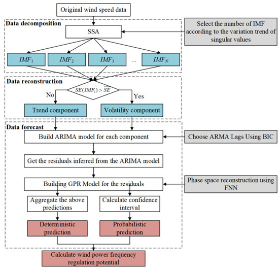
Figure 6.
Framework of hybrid prediction model.
(1) SSA decomposition is performed on the original wind speed series. SSA decomposition yields several modal components with different time-scale fluctuation characteristics. To reduce the complexity of component modeling, the trend component and fluctuation component are obtained by reconstructing the series with the sample entropy as the index.
(2) Modeling and parameter estimation are performed by ARIMA for the reconstructed series, respectively. The trend and fluctuation components are extracted and then the model residuals can be shown as:
where and are the ARIMA (Auto-regressive Integrated Moving Average model) forecasts, respectively; and are the ARIMA model constants for the trend and volatility components, respectively; , , , and are the model orders, respectively; and are the coefficients of the i-th auto-regressive term for the trend and volatility components, respectively; and are the coefficients of the j-th moving average term for the trend and volatility components, respectively.
(3) The residual components are modeled by GPR. In this paper, the reconstruction dimension of the residual modeling is estimated by the False-nearest-neighbors (FNN) algorithm [16], and details of this algorithm can be found in [18]. GPR achieves the prediction of the residuals of the ARIMA model, and the results of the predicted values are superimposed to obtain the final wind speed prediction, which can be expressed as:
where is the prediction obtained from residual et by GPR modeling.
(4) Calculate the probabilistic prediction results. The probabilistic prediction results are obtained by superimposing the GPR prediction residual confidence intervals and the ARIMA prediction results.
(5) The wind power FR potential under the corresponding moment is calculated by deterministic and probabilistic prediction results.
5. Example Analysis
5.1. Deterministic Prediction Evaluation Index
In this paper, the mean absolute percentage error (MAPE), mean absolute error (MAE), and root mean square error (RMSE) are used to quantify the prediction results, aiming to accurately quantify the model performance of different prediction methods from multiple perspectives, which are expressed as follows:
where the true value is represented by .
5.2. Probabilistic Prediction Evaluation Index
The probabilistic prediction results are generally evaluated [19,20] for confidence intervals in the following three dimensions.
(1) The width of the prediction intervals quantified using normalized average width (PINAW) can be expressed as:
where and are the upper and lower limits of the interval under the confidence level; the scaling factor is represented by Q, generally taken as 1.5.
(2) Average coverage error (ACE), this indicator reflects interval reliability and can be expressed as:
ACE can only quantitatively analyze the results for ultra-short-term intervals, and cannot accurately visualize the degree of deviation between the actual values of wind speed and the predicted intervals.
(3) Coverage width-based criterion (CWC) integrates the assessment of interval coverage and interval width, the smaller the CWC the better the probability prediction composite index, expressed as:
5.3. Wind Power FR Potential Forecast
When wind speed is too low, the over-speed standby control is preferred for wind turbines; when the wind speed is too high, pitch control is preferred. Selecting cases close to the critical wind speed can better show the method of this paper.
Therefore, we selected the measured wind speed in September 2015 in a specific area of China as the sample, and the interval of input wind speed was 1 min. Considering the high frequency of data adoption, 720 sampling points were selected for model validation within 12 h. The first 624 sampling points were selected as model training samples, and the last 96 points were selected as test samples.
SSA decomposition is conducted on original wind speed series, and it is found that when the embedding dimension reaches 5, the new modal singular values are basically unchanged, corresponding to the average singular value 1.003, and the decomposition components are divided into trend and fluctuation components, which are modeled by ARIMA, respectively. ARIMA can only model the smooth time series, and the expanded Dickey–Fuller test is applied to estimate the smoothness of the wind speed component. If the original hypothesis is rejected, i.e., there is no unit root, it means that the series is smooth and its difference term d = 0; otherwise, the difference operation is performed on the series until the series is smooth. The parameters in the ARIMA model are estimated using least squares and Bayesian information criterion (BIC). Further deterministic and probabilistic prediction of the residuals is achieved by GPR. Based on the wind speed predictions, the wind power FR potential can be calculated.
In order to verify the effectiveness of the proposed method in wind power frequency regulation potential prediction, the method in this paper is compared with the ARIMA model, SSA-ARIMA model, and SSA-GPR model directly. Assuming that the rated operating wind speed is 12 m/s, the lower limit of wind speed of wind turbine participating in FR operation is 7 m/s, the inherent inertia time constant of wind turbine is 5.04 s, the upper limit of wind turbine speed is 0.7 p.u., and the lower limit is 1.2 p.u. In addition, the fixed deloading level is assumed to be 10%. The results shown in Figure 7 show that the hybrid prediction model proposed in this paper can capture the change trend of the original sequence in the prediction process. Compared with the direct prediction results without sequence decomposition, the prediction accuracy was significantly improved, so as to realize the accurate quantification of wind power FR potential.
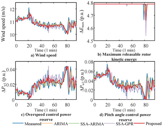
Figure 7.
Deterministic prediction results.
The comparative analysis of the prediction model error performance indexes is shown in Table 1. The evaluation object is set as the prediction accuracy of wind speed. It is not difficult to see that the hybrid prediction model proposed above can accurately realize the crucial feature extraction in the original time series. ARIMA as a linear model has significant advantages in ultra-short-term time series prediction, and GPR can effectively fit the variation of residual nonlinear characteristics. Under different error analysis indexes, the prediction performance of the method in this paper is the best.

Table 1.
Comparison of deterministic prediction model performance.
The probabilistic prediction can reflect the risk information of wind power FR potential prediction results, which may improve the reliability and stability of power system dispatching operation in order to make reasonable decision and dispatching schedule. Figure 8 shows the probabilistic prediction results of wind power FR potential at 99% typical confidence level at a single point in time. It is clear that the proposed method is more detailed and sensitive to the details of probabilistic prediction, and the results of probabilistic prediction at each point in time maintain the appropriate interval width. The confidence interval width can change with the trend of wind speed fluctuation, and has a broader interval width in the significant fluctuation of the target value, which ensures the reliability of the model, and the uncertainty of wind power FR potential is more carefully portrayed.
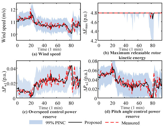
Figure 8.
Probabilistic prediction results.
In terms of probabilistic prediction, SSA-GPR and error statistics methods were selected as the comparison methods. Table 2 gives a comparison of the probabilistic prediction performance, and the proposed methods can maintain relatively excellent performance at all confidence levels, with the smallest uncertainty of PINAW prediction results. The ACE of each probabilistic prediction model is close to 0 with little difference, indicating that different models have good interval coverage. Different confidence levels have a great impact on the model performance of probability prediction. Comparing the comprehensive index CWC, the method in this paper has a smaller CWC as the confidence level decreases, which indicates a stronger robustness and can give full play to the characteristics of GPR in probability prediction such as smaller model bias, good robustness, and wide applicability.
Table 2.
Probabilistic prediction performance.
By setting different reserved deloading levels, the calculated maximum releasable rotor kinetic energy, over-speed control power reserve, and pitch angle control power reserve of wind power are demonstrated in Figure 9.
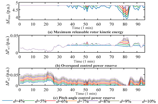
Figure 9.
Wind power frequency regulation potential at different deloading levels.
6. Discussion
Under different wind speeds, different deloading levels have different effects on the frequency regulation potential of wind turbines. It can be seen from the comparison that inertia response capability and primary frequency modulation capability are closely related to time-varying wind speed. In the high wind speed region, due to the speed of the wind turbine being close to the upper limit, the rotor kinetic energy storage margin is sufficient, but at the same time, the over-speed reserve capacity is significantly reduced. In order to realize deloading of wind turbines and power storage of the system, the wind turbine is mainly controlled by pitch control. For scenarios with medium and high wind speed, the storage capacity of wind power is also sufficient, which is stored through over-speed reserve or pitch reserve, and mainly used for deloading reserve through over-speed control. The increase of rotor speed ensures the increase of additional rotor kinetic energy and over-speed reserve capacity. The above analysis shows that rotor kinetic energy storage and over-speed reserve are closely related to wind speed. When the wind speed is high, the over-speed backup control adjustment ability is small. However, compared to pitch control, the response speed of over-speed backup control is fast. The adjustable range of pitch control is large, but response speed is slow.
According to the comparison of the three methods, we can see that the method used in this paper can achieve the best results in PINAW, ACE, and CWC. Taking the CWC index as an example, the proposed method can improve by 0.018 compared with SSA-GPR in the 95-confidence interval.
7. Concluding Remarks
This paper analyzes the wind power participation in system FR basically, considers the effect of different external factors on the wind power FR potential, and discovers dynamic correlations between frequency regulation potential and operating wind speed. On this basis, a prediction model of wind power FR potential is presented along with the following main conclusions.
- For different external wind speeds and reserved deloading levels, the frequency regulation qualifications of wind turbines are different. According to the characteristics of different primary frequency regulation methods, this paper divides the operation areas of over-speed control and pitch control to give full play to the advantages of synergy between the two control strategies.
- Aiming at the wind speed series fluctuation in wind farms, the hybrid model proposed above can better obtain the crucial characteristic components of wind speed series. In addition, the prediction result is better than the traditional method, which improves the prediction accuracy of wind speed series and the evaluation validity of wind power FR potential.
- The proposed probabilistic prediction method of wind power FR potential can complement the accurate deterministic prediction results and respond to uncertain wind power FR potential, based on which the operation and dispatching decision of the grid can be promoted.
Author Contributions
Conceptualization, J.Y.; Formal analysis, X.D.; Methodology, X.D.; Writing—original draft, X.D.; Writing—review & editing, J.Y. All authors have read and agreed to the published version of the manuscript.
Funding
This research received no external funding.
Institutional Review Board Statement
Not applicable.
Informed Consent Statement
Not applicable.
Conflicts of Interest
The authors declare no conflict of interest.
References
- Globalwindreport. [EB/OL]. 2021. Available online: https://gwec.net/global-wind-report-2021 (accessed on 6 April 2022).
- Kumar, M.B.H.; Saravanan, B.; Sanjeevikumar, P.; Blaabjerg, F. Review on control techniques and methodologies for maximum power extraction from wind energy systems. IET Renew. Power Gener. 2018, 12, 1609–1622. [Google Scholar] [CrossRef]
- Godin, P.; Fischer, M.; Röttgers, H.; Mendonca, A.; Engelken, S. Wind power plant level testing of inertial response with optimised recovery behaviour. IET Renew. Power Gener. 2019, 13, 676–683. [Google Scholar] [CrossRef]
- Trovato, V.; Bialecki, A.; Dallagi, A. Unit commitment with inertia-dependent and multispeed allocation of frequency response services. IEEE Trans. Power Syst. 2018, 34, 1537–1548. [Google Scholar] [CrossRef]
- Wang, S.; Tomsovic, K. A novel active power control framework for wind turbine generators to improve frequency response. IEEE Trans. Power Syst. 2018, 33, 6579–6589. [Google Scholar] [CrossRef]
- Fu, Y.; Wang, Y.; Zhang, X. Integrated wind turbine controller with virtual inertia and primary frequency responses for grid dynamic frequency support. IET Renew. Power Gener. 2017, 11, 1129–1137. [Google Scholar] [CrossRef]
- Wu, L.; Infield, D.G. Towards an assessment of power system frequency support from wind plant-modeling aggregate inertial response. IEEE Trans. Power Syst. 2013, 28, 2283–2291. [Google Scholar] [CrossRef]
- Yan, C.; Qin, S.; Zhang, L.; Dai, J.; Tang, Y. Frequency regulation potential prediction of wind power based on historical data. In Proceedings of the 2020 12th IEEE PES Asia-Pacific Power and Energy Engineering Conference (APPEEC), Nanging, China, 20–23 September 2020; pp. 1–5. [Google Scholar]
- Wang, Y.; Bayem, H.; Giralt-Devant, M.; Silva, V.; Guillaud, X.; Francois, B. Methods for assessing available wind primary power reserve. IEEE Trans. Sustain. Energy 2014, 6, 272–280. [Google Scholar] [CrossRef]
- Yan, W.; Cheng, L.; Yan, S.; Gao, W.; Gao, D.W. Enabling and evaluation of inertial control for PMSG-WTG using synchronverter with multiple virtual rotating masses in microgrid. IEEE Trans. Sustain. Energy 2019, 11, 1078–1088. [Google Scholar] [CrossRef]
- Liu, K.; Qu, Y.; Kim, H.M.; Song, H. Avoiding frequency second dip in power unreserved control during wind power rotational speed recovery. IEEE Trans. Power Syst. 2017, 33, 3097–3106. [Google Scholar] [CrossRef]
- Zhang, Z.; Du, E.; Teng, F.; Zhang, N.; Kang, C. Modeling frequency dynamics in unit commitment with a high share of renewable energy. IEEE Trans. Power Syst. 2020, 35, 4383–4395. [Google Scholar] [CrossRef]
- Prieto Cerón, C.E.; Normandia Lourenço, L.F.; Solís-Chaves, J.S.; Sguarezi Filho, A.J. A generalized predictive controller for a wind turbine providing frequency support for a microgrid. Energies 2022, 15, 2562. [Google Scholar] [CrossRef]
- Ochoa, D.; Martinez, S. Analytical approach to understanding the effects of implementing fast-frequency response by wind turbines on the short-term operation of power systems. Energies 2021, 14, 3660. [Google Scholar] [CrossRef]
- Liu, H.; Chen, C. Data processing strategies in wind energy forecasting models and applications: A comprehensive review. Appl. Energy 2019, 249, 392–408. [Google Scholar] [CrossRef]
- Zhang, C.; Wei, H.; Zhao, X.; Liu, T.; Zhang, K. A Gaussian process regression based hybrid approach for short-term wind speed prediction. Energy Convers. Manag. 2016, 126, 1084–1092. [Google Scholar] [CrossRef]
- Richman, J.S.; Moorman, J.R. Physiological time-series analysis using approximate entropy and sample entropy. Am. J. Physiol.-Heart Circ. Physiol. 2000, 278, H2039–H2049. [Google Scholar] [CrossRef] [PubMed] [Green Version]
- Rhodes, C.; Morari, M. False-nearest-neighbors algorithm and noise-corrupted time series. Phys. Rev. E 1997, 55, 6162. [Google Scholar] [CrossRef]
- Khosravi, A.; Nahavandi, S.; Creighton, D. Prediction intervals for short-term wind farm power generation forecasts. IEEE Trans. Sustain. Energy 2013, 4, 602–610. [Google Scholar] [CrossRef]
- Wang, Y.; Hu, Q.; Meng, D.; Zhu, P. Deterministic and probabilistic wind power forecasting using a variational bayesian-based adaptive robust multi-kernel regression model. Appl. Energy 2017, 208, 1097–1112. [Google Scholar] [CrossRef]
Publisher’s Note: MDPI stays neutral with regard to jurisdictional claims in published maps and institutional affiliations. |
© 2022 by the authors. Licensee MDPI, Basel, Switzerland. This article is an open access article distributed under the terms and conditions of the Creative Commons Attribution (CC BY) license (https://creativecommons.org/licenses/by/4.0/).