
Experimental Study on the Thermal Performance of 3D-Printed Enclosing Structures

 ,
, 

Abstract
:1. Introduction
1.1. 3D Printing
1.2. 3D Printing Building Energy Efficiency
1.3. Aim and Tasks
- The evaluation of the thermal resistance coefficient of structures obtained using 3D printing;
- The creation of a mathematical model to describe the process of heat and mass transfer;
- The development and implementation of an experimental bench for validating the proposed mathematical model.
2. Materials and Methods
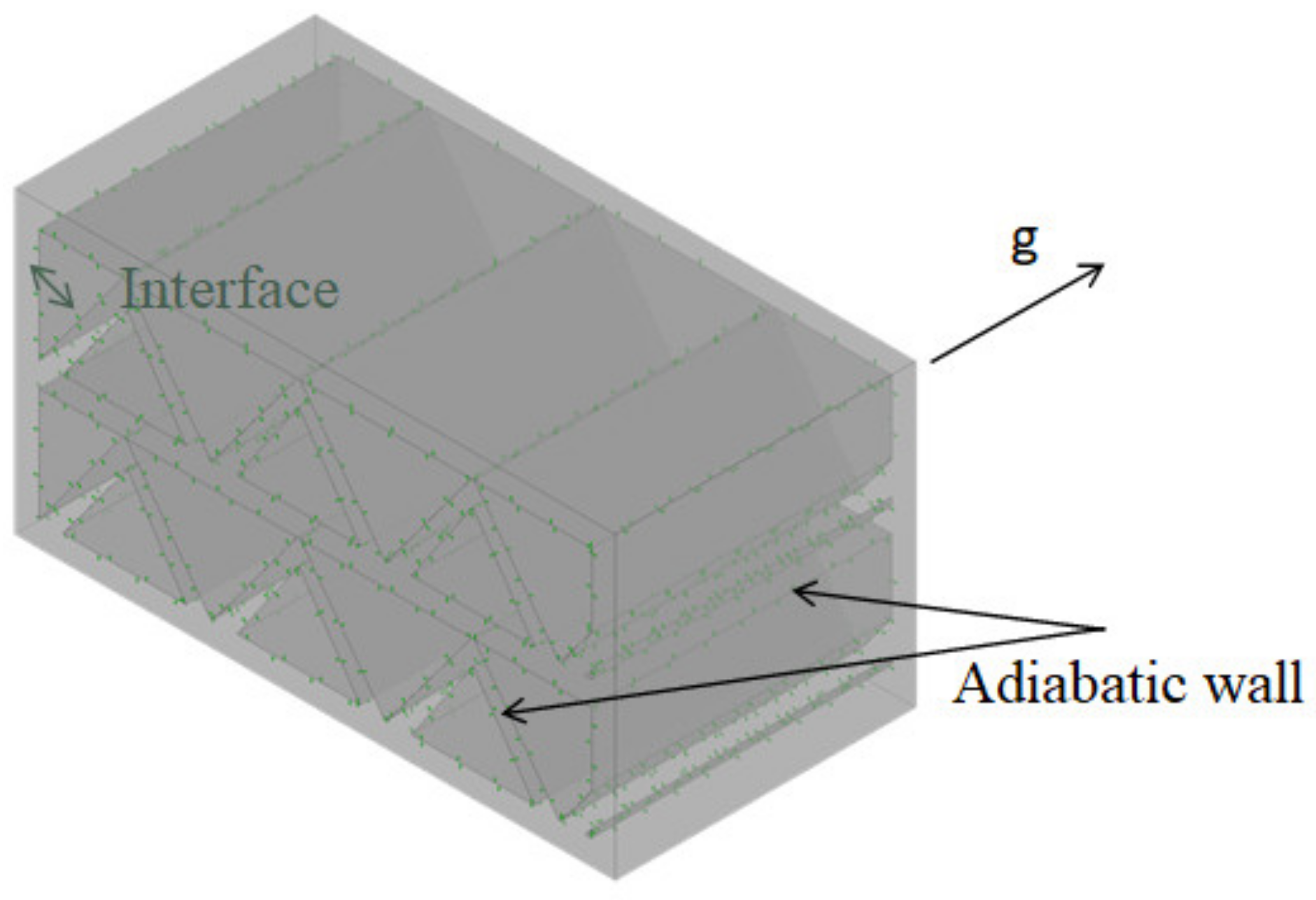
2.1. Problem Statement
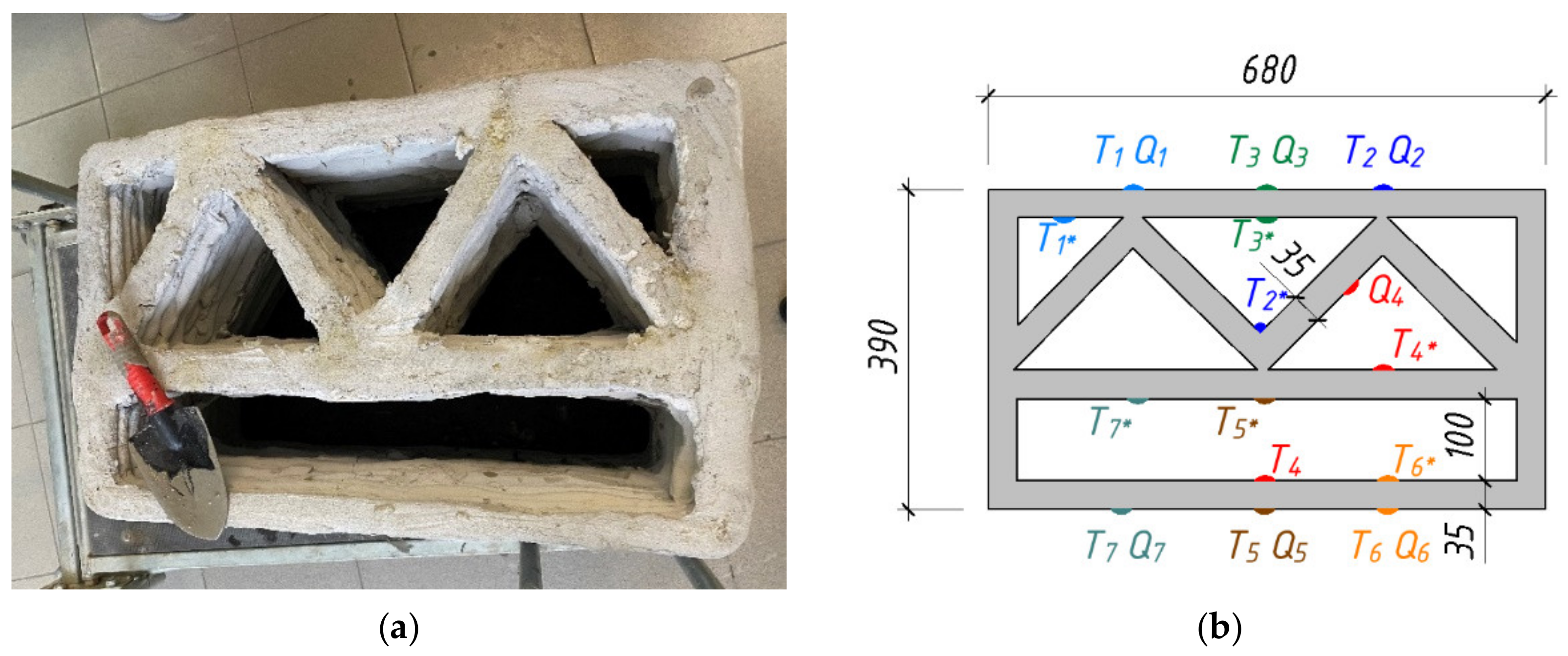
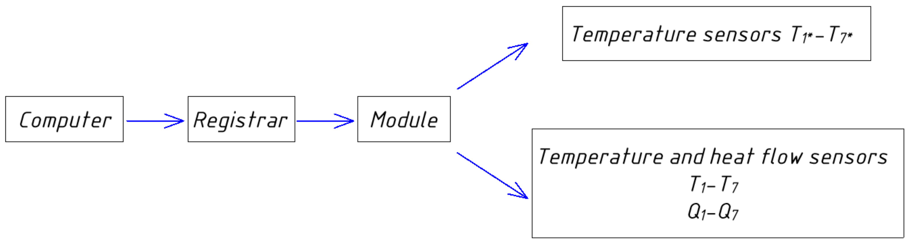
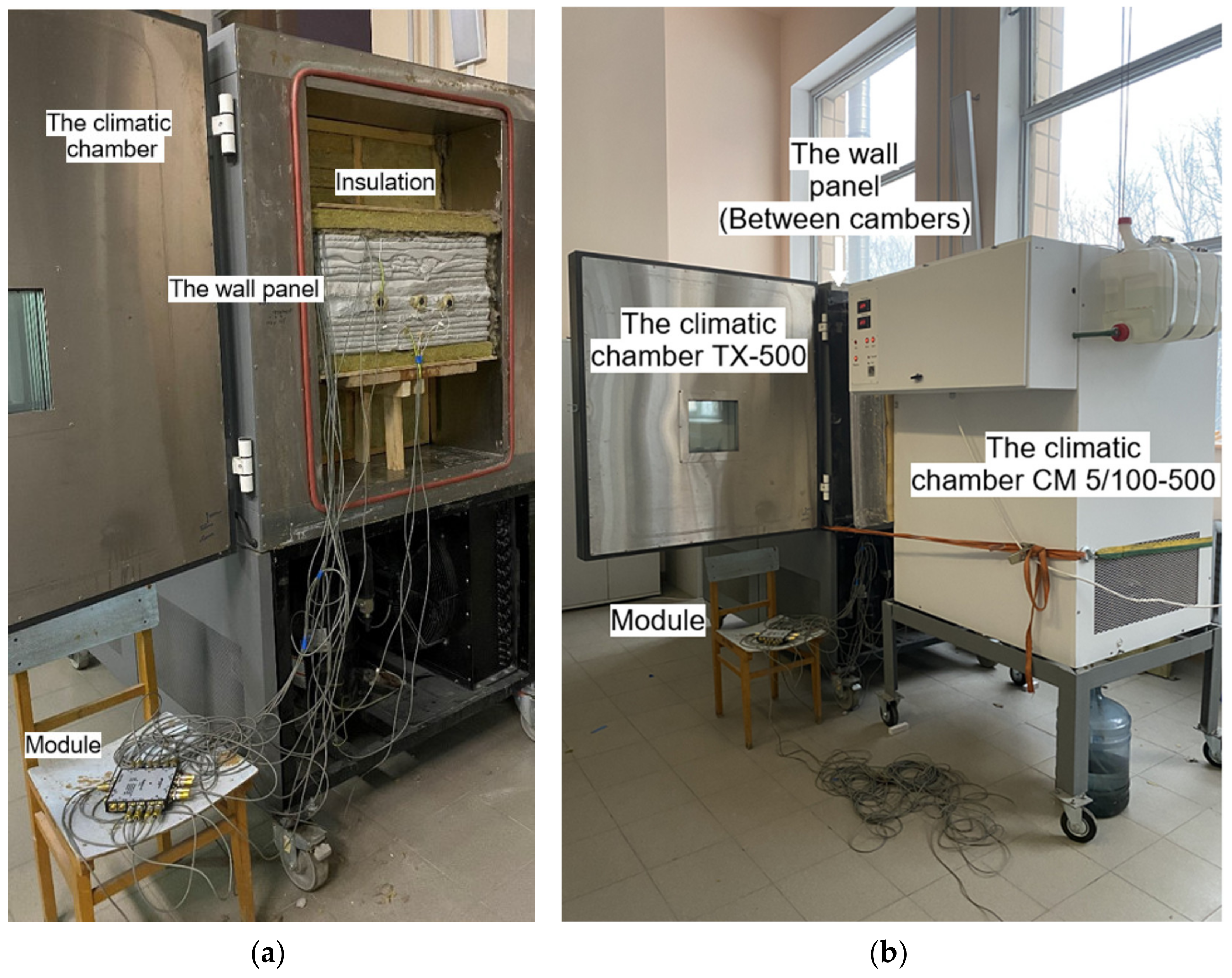
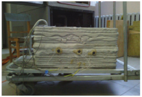
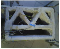
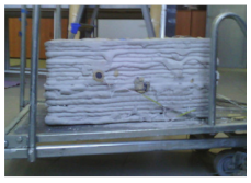
2.2. Experimental Setup
- Climatic chamber No. 1;
- Climatic chamber No. 2;
- The flux density and temperature meter (The technical characteristics are presented in Table 1).
- Compressive strength after 24 h was min 18 MPa;
- Compressive strength after 28 days was min 40 MPa;
- Bending tensile strength after 24 h was min 4 MPa;
- Tensile strength in bending after 28 days was min 8 MPa;
- Waterproof mark was min W14;
- Mark on frost resistance was F600;
- Modulus of elasticity was 26 GPa;
- Climatic zones of application—all zones.
2.3. Numerical Simulation of Heat and Mass Transfer in Enclosing Structures Created by the Method of Additive Technologies
3. Results and Discussion
3.1. Verification and Validation of CFD Simulations
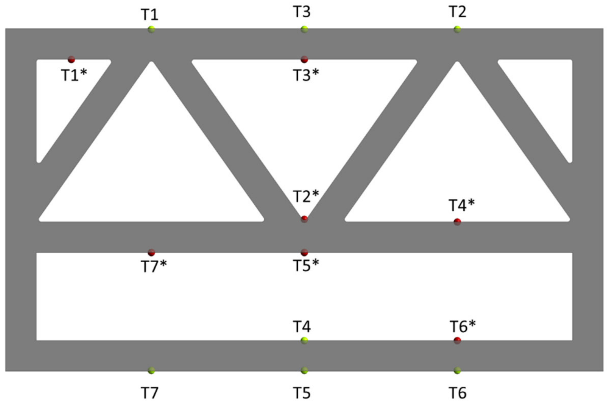
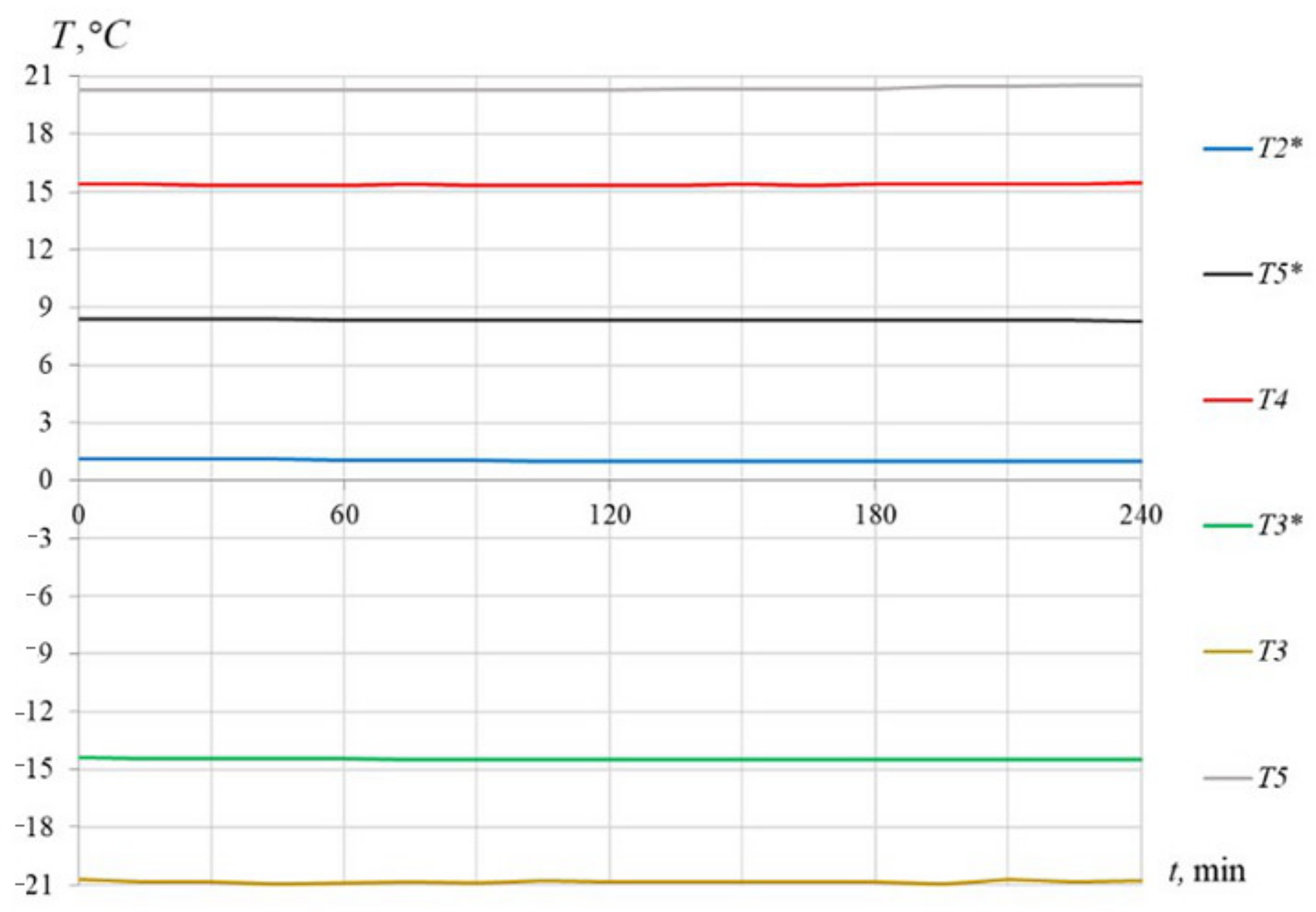
3.1.1. Experimental Results
3.1.2. Estimating Experimental Errors
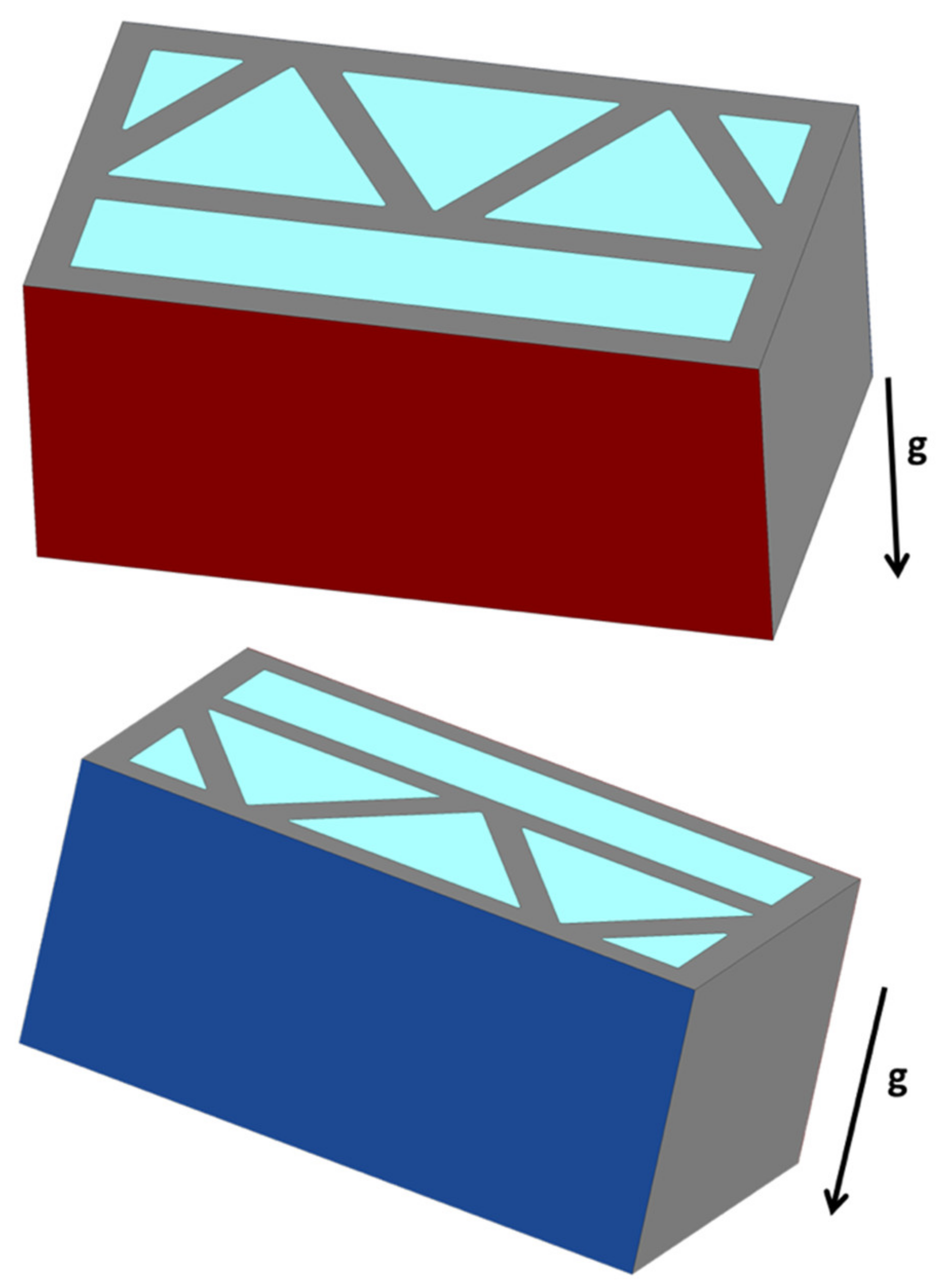
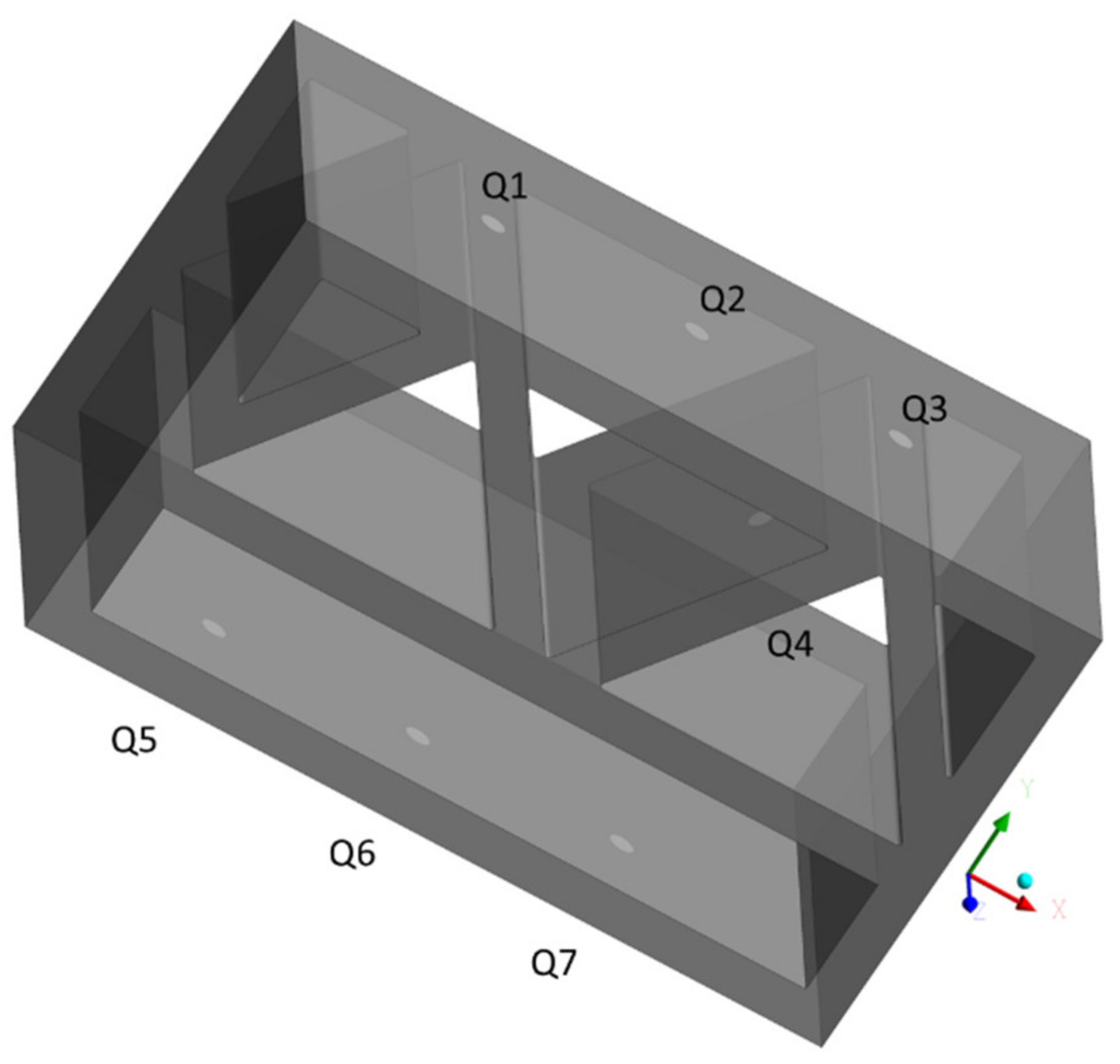
3.1.3. CFD Modeling of the Basic Construction
3.1.4. Verification and Validation of CFD Simulations
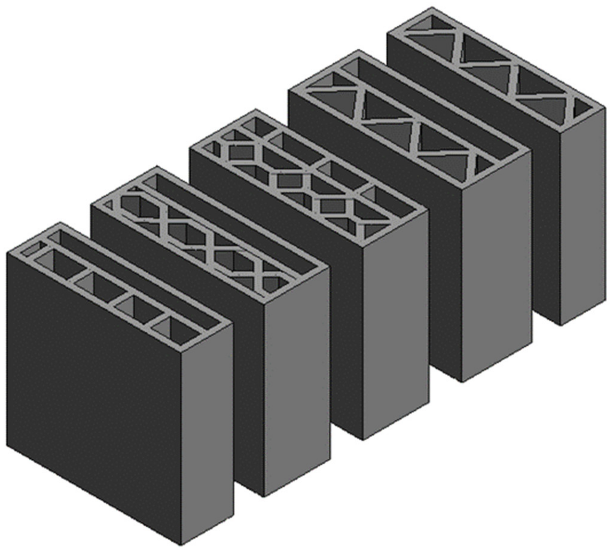
3.2. CFD Simulation of 3D-Printed Constructions with Different Configurations
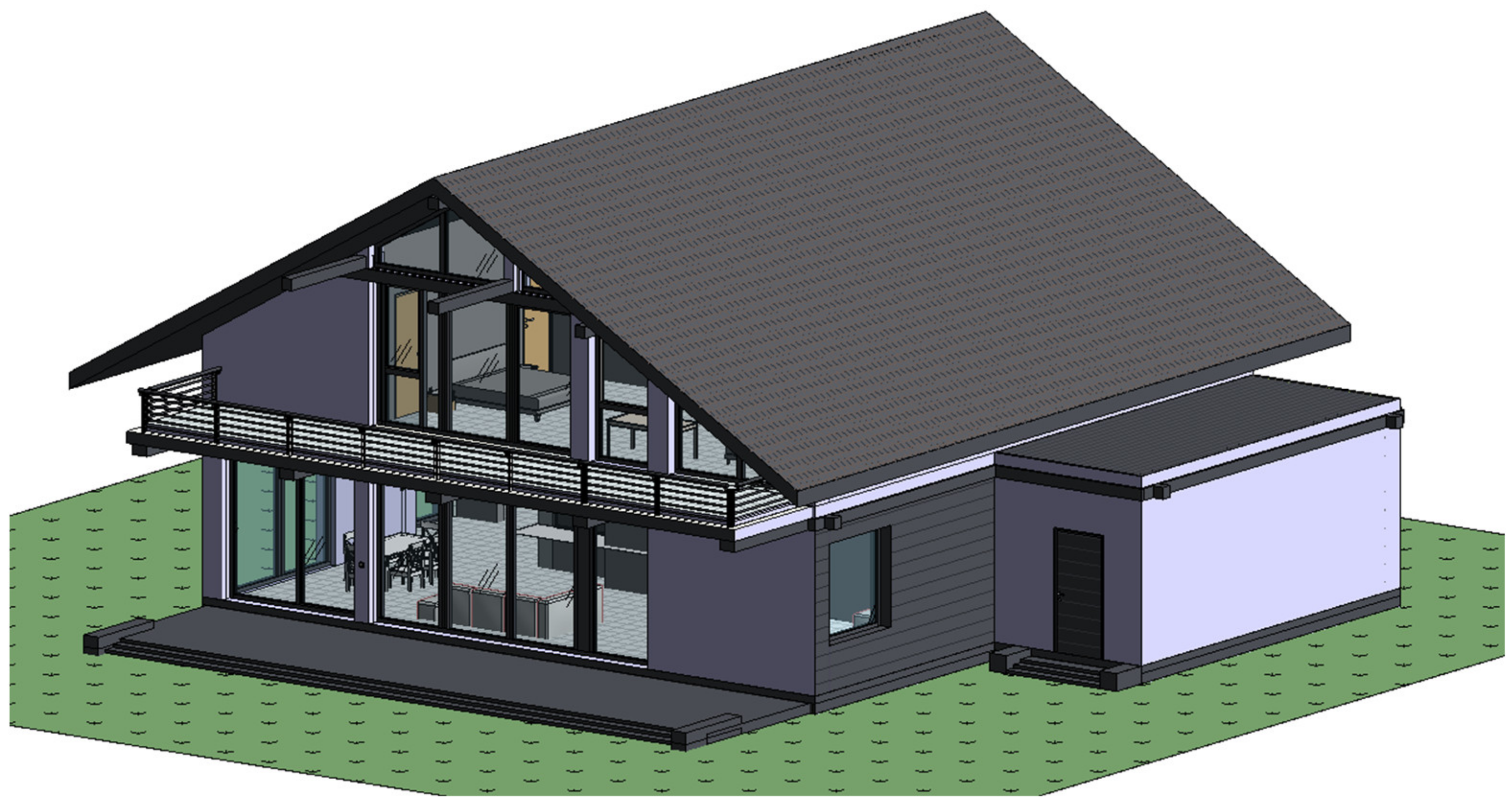
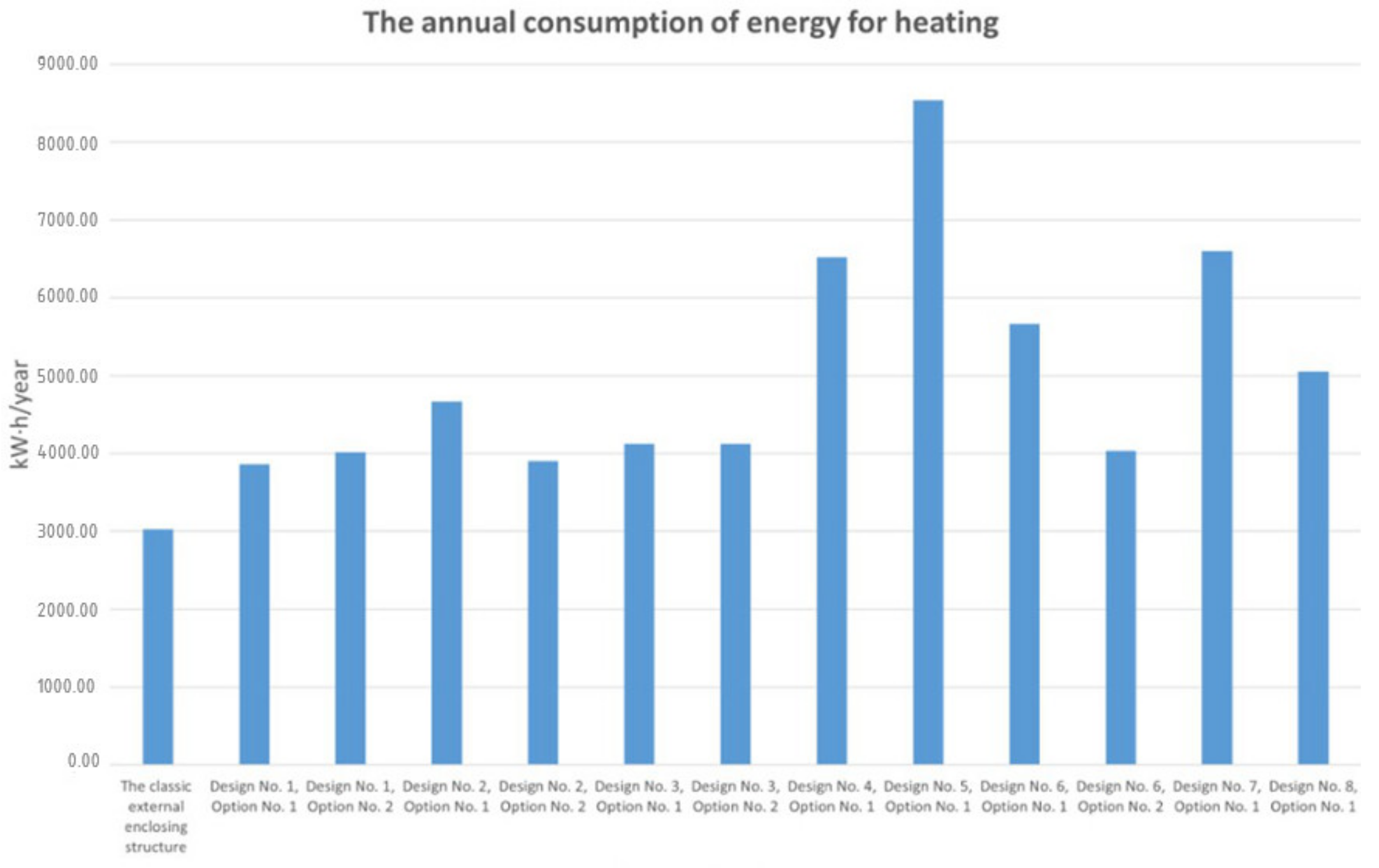
3.3. Energy Modeling Building with 3D-Printed Walls
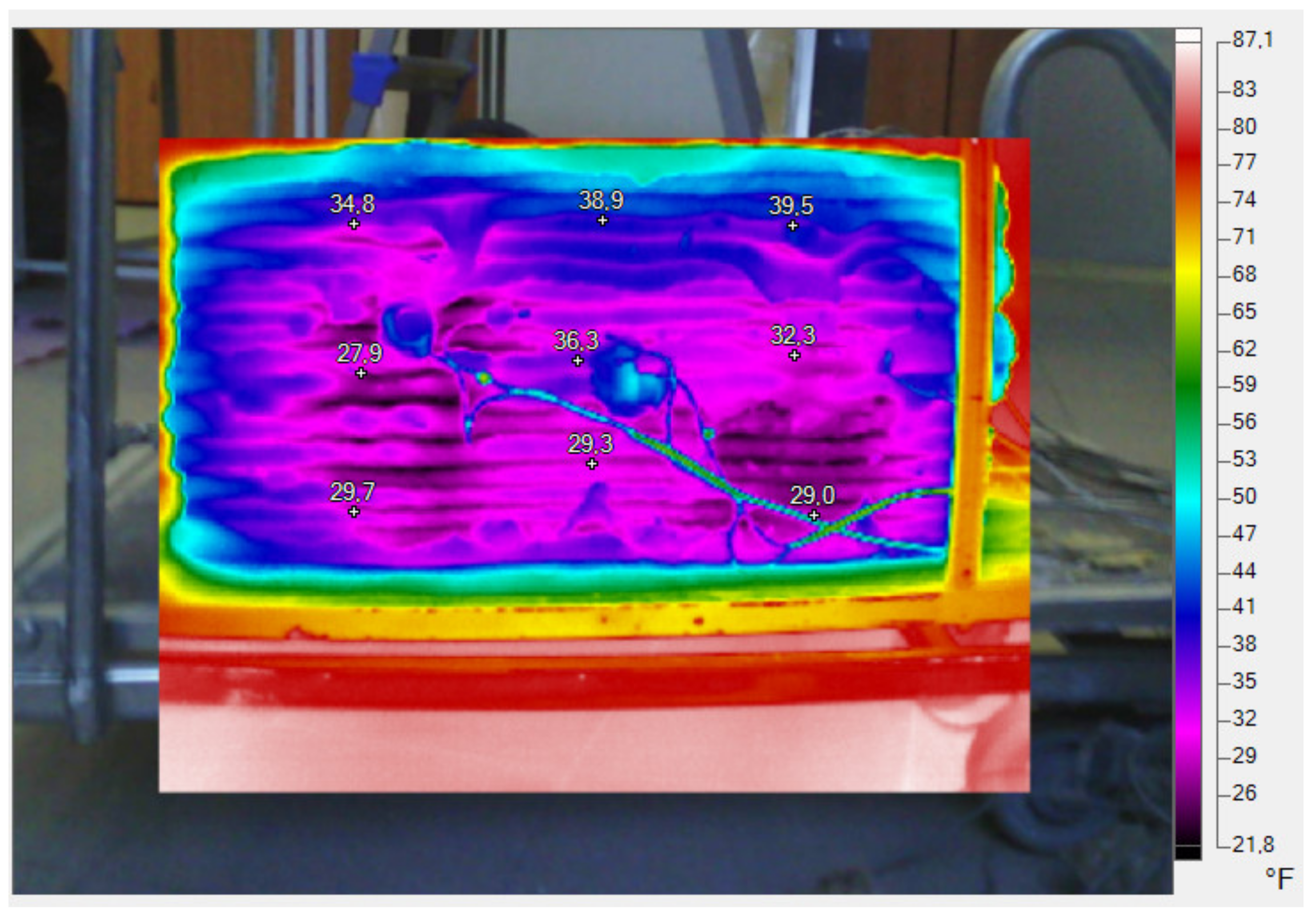
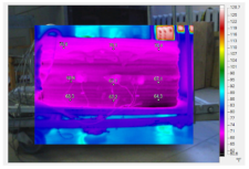
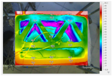
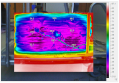
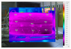
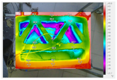
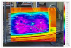
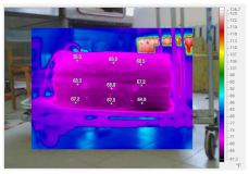
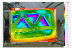
3.4. Thermal Imaging Results
4. Conclusions
- The time of temperature drop in the experimental sample of 3D-printed enclosing structure was determined. The temperature in a cold chamber, Tcold = −24 °C, is dialed within 40 min from the start. For the first 120 min after the start, there is a precipitate drop in the temperature at the sides, δ = 0 mm and δ = 35 mm. The temperature drop occurs mainly inside the structure (δ = 185 mm, δ = 255 mm). After that, the time interval for comparing isotherms is equally more than two hours.
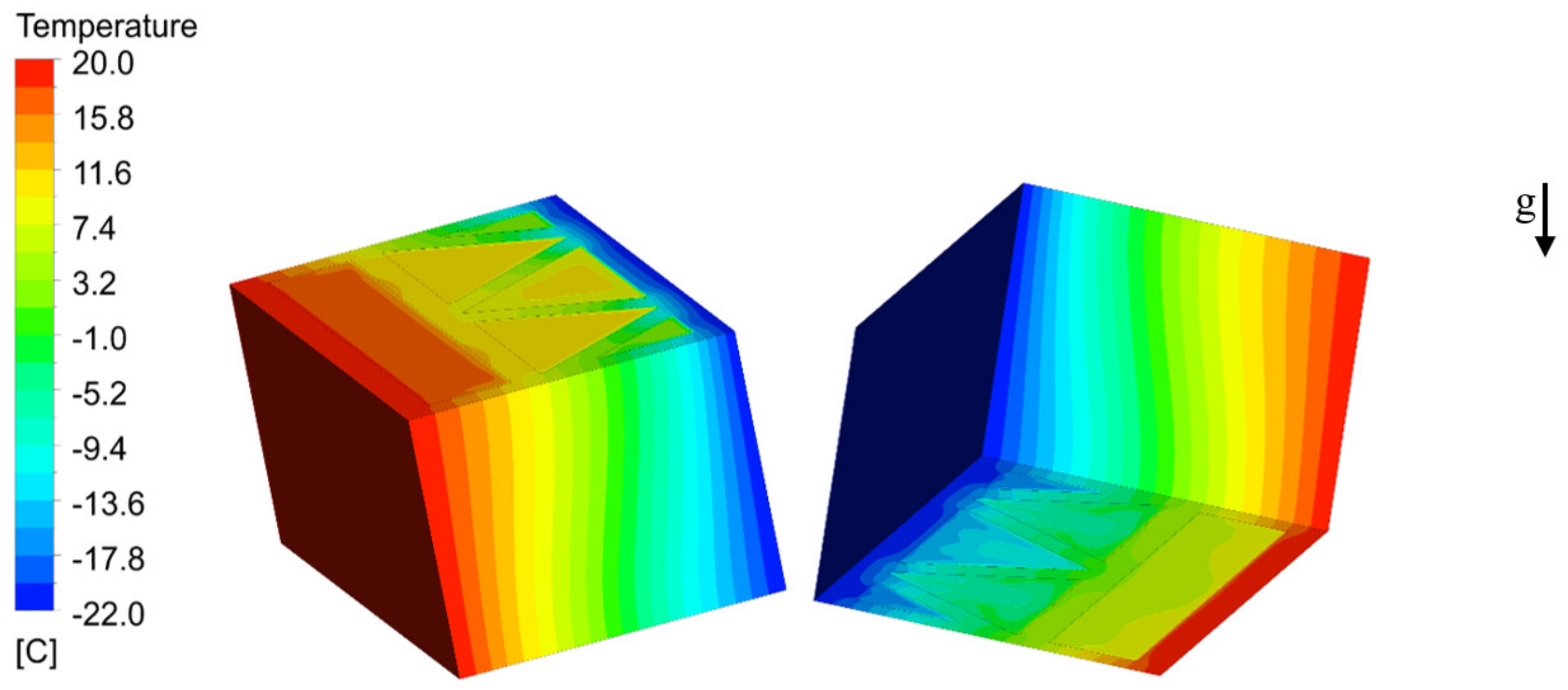
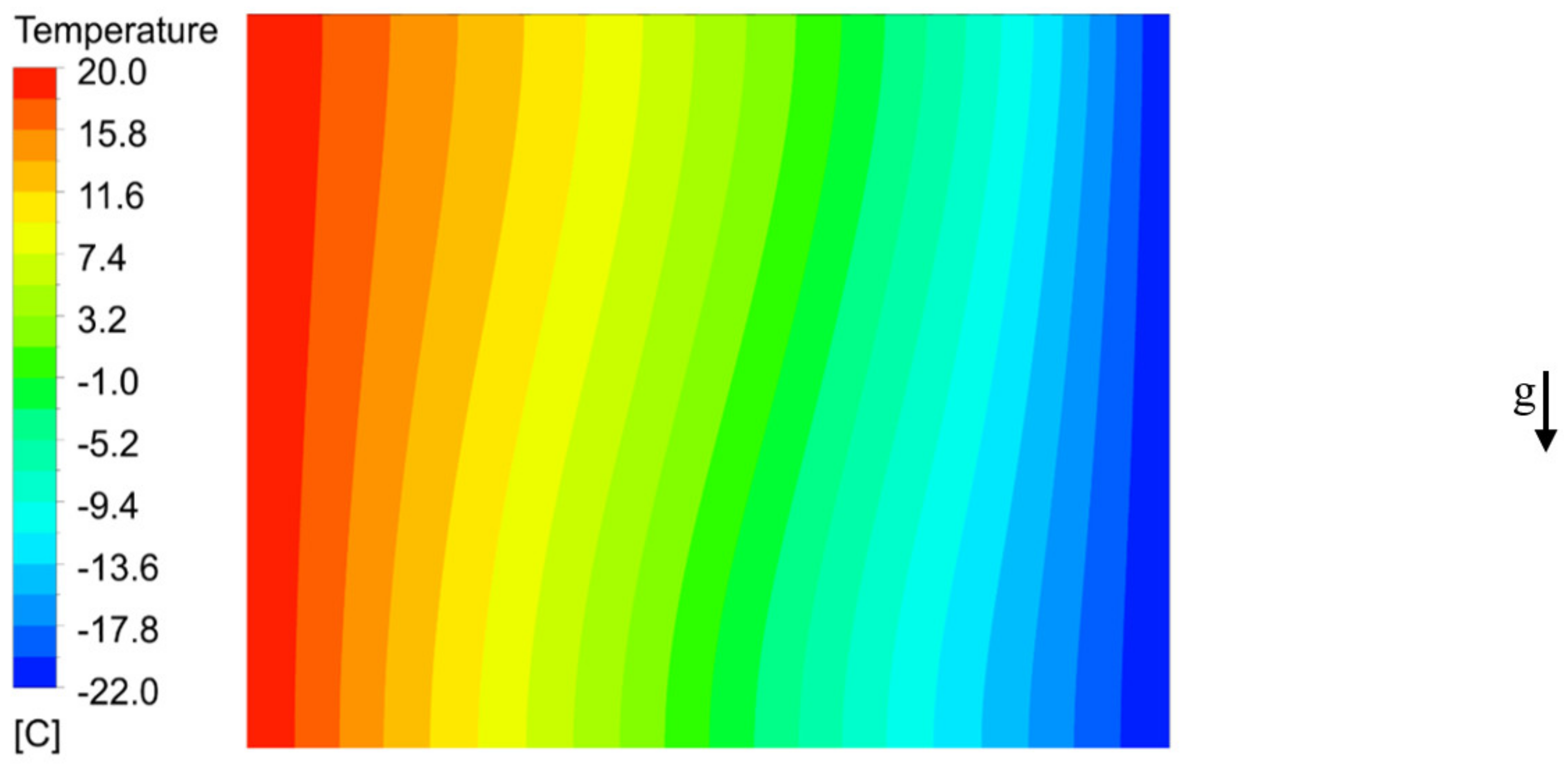
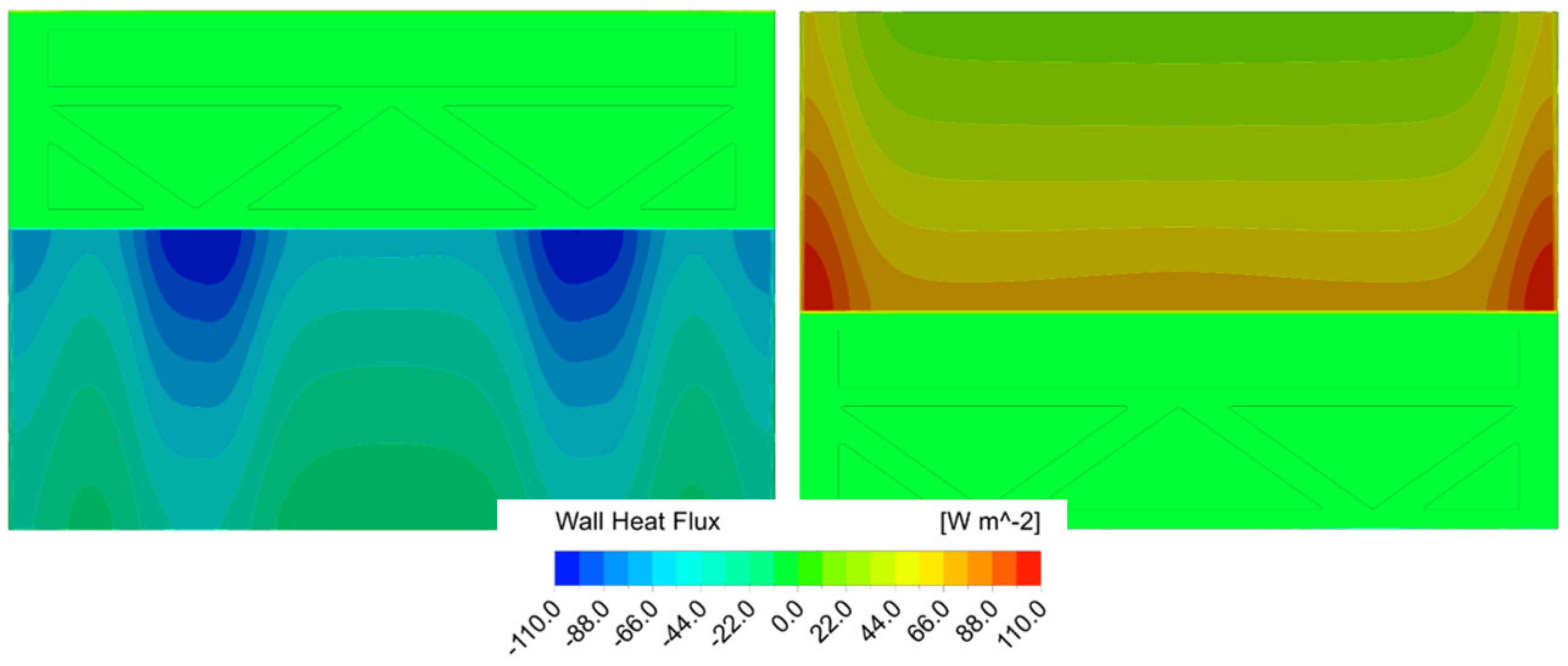
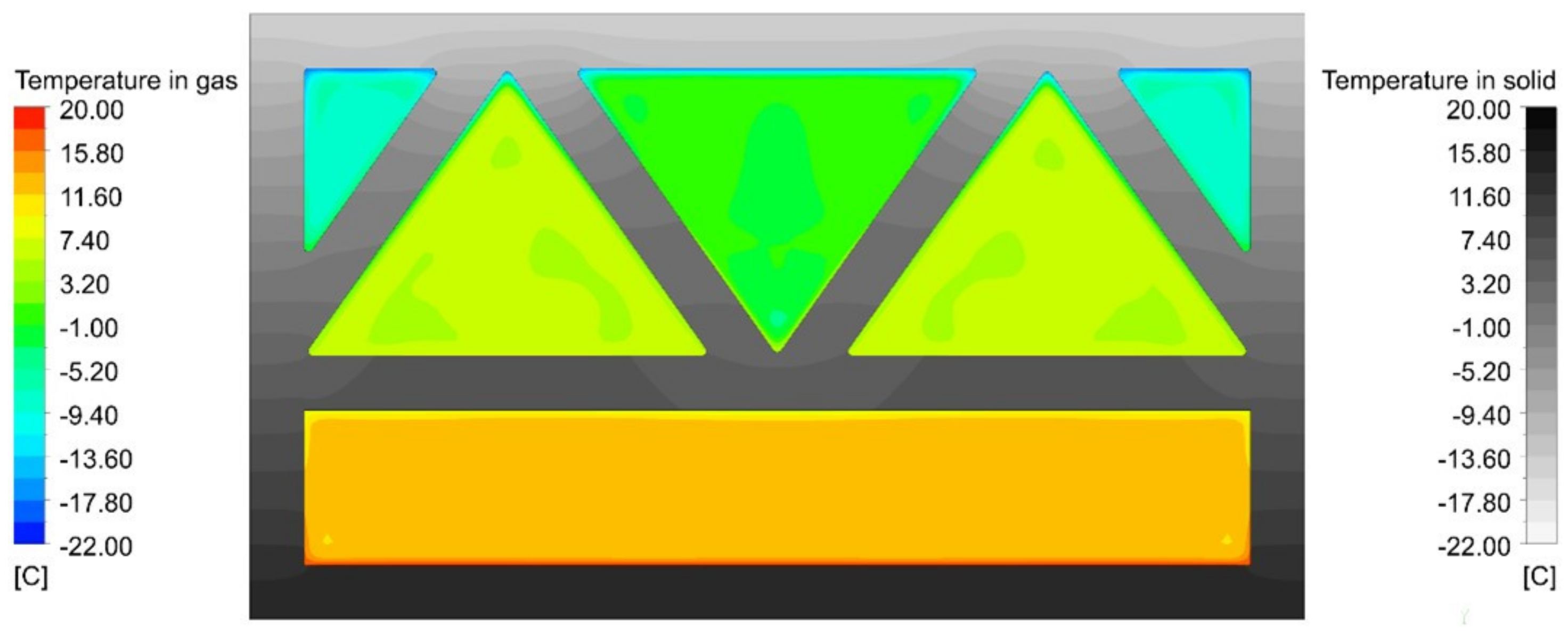
- The CFD modeling of the 3D-printed enclosing structures was also completed. For the basic construction (basic for an experimental sample of 3D-printed enclosing structure), air is hotter on the upper part of the construction than the concrete lintel in the middle, but on the lower part, the air is colder than the lintel. The local temperature difference between concrete and air is around 15 °C.
- The temperature isoline in the 3D-printed enclosing structure becomes more curved while moving the construction’s center from either the hot or cold side. The temperature difference between the lower and the upper sides in the center of the 3D-printed enclosing structure side face is about 5 °C.
- The heat flux through the solid parts of 3D-printed enclosing structures is severely higher (up to 2×) than the heat flux through the air parts of the structures. The convection also influences heat flux distribution on surfaces. If the temperature gradients change because of convection, the heat flux changes (from 100 to 70 W/m2) along the vertical coordinate.
- There is one rectangular cavity, two hot triangle cavities, and three cold rectangular cavities. All cavities except small triangle ones seem to have stabilizing effects on concrete temperature. Noticeable differences in air temperature persist only in boundary layers. The rest of the air volume has an almost constant temperature. The average heat flux through the construction U-value is 1.18.
- The CFD simulation of 3D-printed enclosing structures with different configurations was obtained. Convection in the 3D-printed enclosing structures can add some heat resistance (Table 7) compared to the empirical approach (as it was in geometries 1–3 and 8) and make it not better (as it was in geometries 4–7). Convection works better for more uneven cavern distributions. Empirical formulas give lower U-values, which are unacceptable for engineering purposes for variants with insulation.
- Energy modeling of the building with 3D-printed enclosing structures with different construction configurations was conducted. The annual energy consumption of the 3D-printed building with different construction configurations of 3D-printed enclosing structures is between 3026 and 8536 kW·h per year.
- Thermal imaging results showed the presence of surface irregularities. These thermal inclusions require further research of inhomogeneities, thermal inclusions for structures developed by additive technologies, on the thermal properties of these structures.
Author Contributions
Funding
Institutional Review Board Statement
Informed Consent Statement
Data Availability Statement
Acknowledgments
Conflicts of Interest
References
- Suntharalingam, T.; Gatheeshgar, P.; Upasiri, I.; Poologanathan, K.; Nagaratnam, B.; Rajanayagam, H.; Navaratnam, S. Numerical Study of Fire and Energy Performance of Innovative Light-Weight 3d Printed Concrete Wall Configurations in Modular Building System. Sustainability 2021, 13, 2314. [Google Scholar] [CrossRef]
- He, Y.; Zhang, Y.; Zhang, C.; Zhou, H. Energy-Saving Potential of 3D Printed Concrete Building with Integrated Living Wall. Energy Build. 2020, 222, 110110. [Google Scholar] [CrossRef]
- Yang, S.; Wi, S.; Park, J.H.; Cho, H.M.; Kim, S. Novel Proposal to Overcome Insulation Limitations Due to Nonlinear Structures Using 3D Printing: Hybrid Heat-Storage System. Energy Build. 2019, 197, 177–187. [Google Scholar] [CrossRef]
- Robati, M.; McCarthy, T.J.; Kokogiannakis, G. Incorporating Environmental Evaluation and Thermal Properties of Concrete Mix Designs. Constr. Build. Mater. 2016, 128, 422–435. [Google Scholar] [CrossRef] [Green Version]
- Prasittisopin, L.; Pongpaisanseree, K.; Jiramarootapong, P.; Snguanyat, C. Thermal and Sound Insulation of Large-Scale 3D Extrusion Printing Wall Panel; Springer: Cham, Switzerland, 2020; Volume 28, pp. 1174–1182. [Google Scholar] [CrossRef]
- Alkhalidi, A.; Hatuqay, D. Energy Efficient 3D Printed Buildings: Material and Techniques Selection Worldwide Study. J. Build. Eng. 2020, 30, 101286. [Google Scholar] [CrossRef]
- González-Torres, M.; Pérez-Lombard, L.; Coronel, J.F.; Maestre, I.R.; Yan, D. A Review on Buildings Energy Information: Trends, End-Uses, Fuels and Drivers. Energy Rep. 2022, 8, 626–637. [Google Scholar] [CrossRef]
- Marais, H.; Christen, H.; Cho, S.; de Villiers, W.; van Zijl, G. Computational Assessment of Thermal Performance of 3D Printed Concrete Wall Structures with Cavities. J. Build. Eng. 2021, 41, 102431. [Google Scholar] [CrossRef]
- Thakur, N.; Prasath Kumar, V.R.; Balasubramanian, M. Comparative Energy Audit of Building Models Using BIM for the Sustainable Development. J. Adv. Res. Dyn. Control Syst. 2018, 10, 986–992. [Google Scholar]
- Singh, P.; Sadhu, A. Multicomponent Energy Assessment of Buildings Using Building Information Modeling. Sustain. Cities Soc. 2019, 49, 101603. [Google Scholar] [CrossRef]
- Ajayi, S.O.; Oyedele, L.O.; Ilori, O.M. Changing Significance of Embodied Energy: A Comparative Study of Material Specifications and Building Energy Sources. J. Build. Eng. 2019, 23, 324–333. [Google Scholar] [CrossRef] [Green Version]
- Olanrewaju, S.D.; Adetunji, O.S.; Ogundepo, T.M. Achieving Energy Efficient Building through Energy Performance Analysis of Building Envelope in Student Housing. J. Phys. Conf. Ser. 2019, 1378, 042023. [Google Scholar] [CrossRef]
- Bhamare, D.K.; Rathod, M.K.; Banerjee, J. Numerical Model for Evaluating Thermal Performance of Residential Building Roof Integrated with Inclined Phase Change Material (PCM) Layer. J. Build. Eng. 2020, 28, 101018. [Google Scholar] [CrossRef]
- Shen, S.; Kanbur, B.B.; Zhou, Y.; Duan, F. Thermal and Mechanical Assessments of the 3D-Printed Conformal Cooling Channels: Computational Analysis and Multi-Objective Optimization. J. Mater. Eng. Perform. 2020, 29, 8261–8270. [Google Scholar] [CrossRef]
- Kanbur, B.B.; Shen, S.; Zhou, Y.; Duan, F. Thermal and Mechanical Simulations of the Lattice Structures in the Conformal Cooling Cavities for 3D Printed Injection Molds. Mater. Today Proc. 2019, 28, 379–383. [Google Scholar] [CrossRef]
- Khan, S.A.; Koç, M.; Al-Ghamdi, S.G. Sustainability Assessment, Potentials and Challenges of 3D Printed Concrete Structures: A Systematic Review for Built Environmental Applications. J. Clean. Prod. 2021, 303, 127027. [Google Scholar] [CrossRef]
- Amran, M.; Abdelgader, H.S.; Onaizi, A.M.; Fediuk, R.; Ozbakkaloglu, T.; Rashid, R.S.M.; Murali, G. 3D-Printable Alkali-Activated Concretes for Building Applications: A Critical Review. Constr. Build. Mater. 2022, 319, 126126. [Google Scholar] [CrossRef]
- Pan, Y.; Zhang, Y.; Zhang, D.; Song, Y. 3D Printing in Construction: State of the Art and Applications. Int. J. Adv. Manuf. Technol. 2021, 115, 1329–1348. [Google Scholar] [CrossRef]
- Craveiro, F.; Bartolo, H.M.; Gale, A.; Duarte, J.P.; Bartolo, P.J. A Design Tool for Resource-Efficient Fabrication of 3d-Graded Structural Building Components Using Additive Manufacturing. Autom. Constr. 2017, 82, 75–83. [Google Scholar] [CrossRef] [Green Version]
- Harmati, N.; Jakšić, Ž.; Vatin, N. Energy Consumption Modelling via Heat Balance Method for Energy Performance of a Building. Procedia Eng. 2015, 117, 786–794. [Google Scholar] [CrossRef] [Green Version]
- Lee, Y.H.; Chua, N.; Amran, M.; Lee, Y.Y.; Kueh, A.B.H.; Fediuk, R.; Vatin, N.; Vasilev, Y. Thermal Performance of Structural Lightweight Concrete Composites for Potential Energy Saving. Crystals 2021, 11, 461. [Google Scholar] [CrossRef]
- Klyuev, S.V.; Klyuev, A.V.; Vatin, N.I.; Shorstova, E.S. Technology of 3-d Printing of Fiber Reinforced Mixtures; Springer: Cham, Switzerland, 2021; Volume 141, pp. 224–230. [Google Scholar] [CrossRef]
- Nair, A.; Aditya, S.D.; Adarsh, R.N.; Nandan, M.; Dharek, M.S.; Sreedhara, B.M.; Prashant, S.C.; Sreekeshava, K.S. Additive Manufacturing of Concrete: Challenges and Opportunities. IOP Conf. Ser. Mater. Sci. Eng. 2020, 814, 012022. [Google Scholar] [CrossRef]
- Nazarian, S.; Duarte, J.P.; Bilén, S.G.; Memari, A.; Radlinska, A.; Meisel, N.; Hojati, M. Additive Manufacturing of Architectural Structures: An Interplay Between Materials, Systems, and Design. In Sustainability and Automation in Smart Constructions. Advances in Science, Technology & Innovation; Rodrigues, H., Gaspar, F., Fernandes, P., Mateus, A., Eds.; Springer: Cham, Switzerland, 2021; pp. 111–119. [Google Scholar] [CrossRef]
- Buswell, R.A.; Leal de Silva, W.R.; Jones, S.Z.; Dirrenberger, J. 3D Printing Using Concrete Extrusion: A Roadmap for Research. Cem. Concr. Res. 2018, 112, 37–49. [Google Scholar] [CrossRef]
- Dobrzyńska, E.; Kondej, D.; Kowalska, J.; Szewczyńska, M. State of the Art in Additive Manufacturing and Its Possible Chemical and Particle Hazards—Review. Indoor Air 2021, 31, 1733–1758. [Google Scholar] [CrossRef]
- Gosselin, C.; Duballet, R.; Roux, P.; Gaudillière, N.; Dirrenberger, J.; Morel, P. Large-Scale 3D Printing of Ultra-High Performance Concrete—A New Processing Route for Architects and Builders. Mater. Des. 2016, 100, 102–109. [Google Scholar] [CrossRef] [Green Version]
- Lowke, D.; Dini, E.; Perrot, A.; Weger, D.; Gehlen, C.; Dillenburger, B. Particle-Bed 3D Printing in Concrete Construction—Possibilities and Challenges. Cem. Concr. Res. 2018, 112, 50–65. [Google Scholar] [CrossRef]
- Vatin, N.I.; Gorshkov, A.S.; Nemova, D.V. Energy Efficiency of Envelopes at Major Repairs. Constr. Unique Build. Struct. 2013, 3, 1–11. [Google Scholar]
- Sergeev, V.; Vatin, N.; Kotov, E.; Nemova, D.; Khorobrov, S. Slug regime transitions in a two-phase flow in horizontal round pipe. cfd simulations. Appl. Sci. 2020, 10, 8739. [Google Scholar] [CrossRef]
- Buswell, R.A.; Thorpe, A.; Soar, R.C.; Gibb, A.G.F. Design, Data and Process Issues for Mega-Scale Rapid Manufacturing Machines Used for Construction. Autom. Constr. 2008, 17, 923–929. [Google Scholar] [CrossRef] [Green Version]
- Buswell, R.A.; Soar, R.C.; Gibb, A.G.F.; Thorpe, A. Freeform Construction: Mega-Scale Rapid Manufacturing for Construction. Autom. Constr. 2007, 16, 224–231. [Google Scholar] [CrossRef] [Green Version]
- Saracoglu, A.; Sanli, D.U. Accuracy of GPS Positioning Concerning Köppen-Geiger Climate Classification. Measurement 2021, 181, 109629. [Google Scholar] [CrossRef]


| Characteristic | Value |
|---|---|
| Measuring the range of heat flux density, W/m2 | 10–500 |
| Temperature measurement ranges, °C | −40 °C–+70 °C |
| Limits of the permissible basic relative error of measuring the heat flux density, %, no more | ±6 |
| Limits of the permissible basic absolute error of temperature measurement, °C | ±0.2 |
| Density | Viscosity | Specific Heat | Thermal Conductivity | Molar Mass | |
|---|---|---|---|---|---|
| kg/m3 | Pa·s | J/(kg·K) | W/(m·K) | g/mol | |
| Air | ideal gas | 1.83 × 10⁻⁵ | 1004.4 | 0.0261 | 28.96 |
| Concrete | 1900 | - | 1130 | 0.7 | - |
| n | The Temperature in Steady-State Mode | Average Value | Standard Deviation | Error | ||
|---|---|---|---|---|---|---|
| Day 1 | Day 2 | Day 3 | ||||
| T3 | −20.84 | −20.34 | −20.48 | −20.59 | 0.2579 | 1.25% |
| T3* | −14.48 | −14.3 | −14.6 | −14.39 | 0.1510 | 1.05% |
| T2* | 1.04 | 1.04 | 1.05 | 1.04 | 0.0058 | 0.56% |
| T5* | 8.33 | 8.58 | 8.32 | 8.455 | 0.1468 | 1.74% |
| T4 | 15.37 | 15.04 | 14.81 | 15.205 | 0.2793 | 1.84% |
| T5 | 20.35 | 20.45 | 20.41 | 20.4 | 0.0501 | 0.25% |
| Temperature T, °C | |||||||
|---|---|---|---|---|---|---|---|
| Sensor No. | Exp1 | Exp2 | Exp3 | Comp | Diff1 | Diff2 | Diff3 |
| 1 | −22.14 | −22.43 | −22.5 | −21.800 | 1.6% | 2.9% | 3.0% |
| 2 | −21.27 | −21.50 | −22 | −21.800 | 2.5% | 1.4% | 0.9% |
| 3 | −20.92 | −21.34 | −21.5 | −21.880 | 4.5% | 2.5% | 1.9% |
| 4 | 15.07 | 15.04 | 14.81 | 15.820 | 4.9% | 5.0% | 6.6% |
| 5 | 20.50 | 20.45 | 20.41 | 19.960 | 2.7% | 2.4% | 2.2% |
| 6 | 19.88 | 20.23 | 20.18 | 19.960 | 0.4% | 1.4% | 1.1% |
| 7 | 20.49 | 20.39 | 20.34 | 19.960 | 2.6% | 2.1% | 1.9% |
| Temperature T, °C | |||||||
|---|---|---|---|---|---|---|---|
| Sensor No. | Exp1 | Exp2 | Exp3 | Comp | Diff1 | Diff2 | Diff3 |
| 1 | −11.82 | −11.34 | −11.1 | −11.020 | 7.0% | 2.8% | 0.7% |
| 2 | 1.21 | 0.04 | −0.33 | 0.19 | 146.0% | 131.7% | 743.2% |
| 3 | −14.23 | −15.30 | −15.6 | −15.000 | 5.3% | 2.0% | 3.9% |
| 4 | 3.63 | 3.08 | 2.482 | 3.889 | 6.8% | 23.1% | 44.2% |
| 5 | 8.28 | 7.58 | 7.322 | 7.947 | 4.1% | 4.7% | 8.2% |
| 6 | 14.56 | 14.66 | 14.4 | 15.630 | 7.1% | 6.4% | 8.2% |
| 7 | 9.16 | 8.46 | 8.307 | 8.568 | 6.7% | 1.2% | 3.1% |
| Average Heat Flux, W/m2 | |||||||
|---|---|---|---|---|---|---|---|
| Sensor No. | Exp1 | Exp2 | Exp3 | Comp | Diff1 | Diff2 | Diff3 |
| 1 | 48.57 | 44.11 | 43.59 | 72.33 | 39.3% | 48.5% | 49.6% |
| 2 | 77.40 | 71.57 | 72.45 | 72.51 | 6.5% | 1.3% | 0.1% |
| 3 | 26.24 | 24.46 | 23.52 | 30.88 | 16.2% | 23.2% | 27.0% |
| 4 | 18.32 | 22.82 | 22.16 | 23.16 | 23.3% | 1.5% | 4.4% |
| 5 | 23.50 | 18.78 | 19.07 | 39.88 | 51.7% | 71.9% | 70.6% |
| 6 | 27.46 | 19.25 | 19.42 | 40.10 | 37.4% | 70.3% | 69.5% |
| 7 | 30.46 | 24.53 | 25.35 | 40.10 | 27.3% | 48.2% | 45.1% |
| Characteristic | Construction Cross-Section View | ||
|---|---|---|---|
| 1 |  | 1.03 | 0.89 |
| 2 |  | 1.37 | 1.05 |
| 3 | 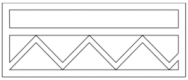 | 1.52 | 1.15 |
| 4 | 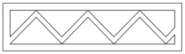 | 2.13 | 2.00 |
| 5 | 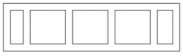 | 2.38 | 3.03 |
| 6 | 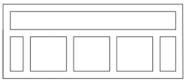 | 1.52 | 1.59 |
| 7 |  | 2.08 | 2.04 |
| 8 | 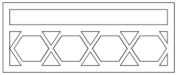 | 1.49 | 1.25 |
| Characteristic | Construction Cross-Section View | ||
|---|---|---|---|
| 1 |  | 0.33 | 0.48 |
| 2 | 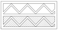 | 0.33 | 0.66 |
| 3 | 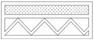 | 0.28 | 0.78 |
| 4 | 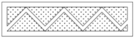 | 0.36 | 1.12 |
| 5 | 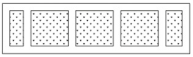 | 1.10 | 1.10 |
| 6 | 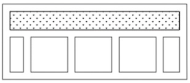 | 0.40 | 0.73 |
| 7 |  | 0.37 | 1.03 |
| 8 |  | 0.31 | 1.19 |
| Type of Enclosing Structure | Construction Area, Ai, m2 | The Coefficient of Heat Transmission, U, W/m2∙°C |
|---|---|---|
| Roof | 264.45 | 0.22 |
| Stained-glass panels and balcony doors | 89.28 | 1.33 |
| External entrance doors | 16.88 | 1.11 |
| Foundation slab and floor | 211 | 0.23 |
| Type of external enclosing structure | ||
| The classic external enclosing structure | 182.23 | 0.21 |
Design No. 1, Option No. 1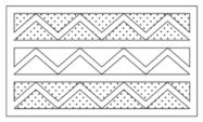 | 182.23 | 0.64 |
Design No. 1, Option No. 2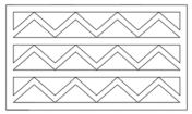 | 182.23 | 0.72 |
Design No. 2, Option No. 1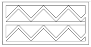 | 182.23 | 1.05 |
Design No. 2, Option No. 2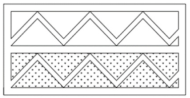 | 182.23 | 0.66 |
Design No. 3, Option No. 1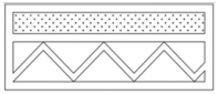 | 182.23 | 0.78 |
Design No. 3, Option No. 2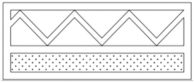 | 182.23 | 0.78 |
Design No. 4, Option No. 1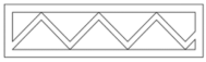 | 182.23 | 2 |
Design No. 5, Option No. 1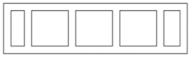 | 182.23 | 3.03 |
Design No. 6, Option No. 1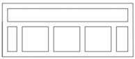 | 182.23 | 1.56 |
Design No. 6, Option No. 2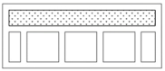 | 182.23 | 0.73 |
Design No. 7, Option No. 1 | 182.23 | 2.04 |
Design No. 8, Option No. 1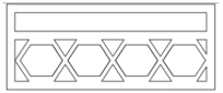 | 182.23 | 1.25 |
| Front of the Panel | Top View of the Panel | Back of the Panel |
|---|---|---|
 |  |  |
 |  |  |
 |  |  |
 |  |  |
Publisher’s Note: MDPI stays neutral with regard to jurisdictional claims in published maps and institutional affiliations. |
© 2022 by the authors. Licensee MDPI, Basel, Switzerland. This article is an open access article distributed under the terms and conditions of the Creative Commons Attribution (CC BY) license (https://creativecommons.org/licenses/by/4.0/).
Share and Cite
Nemova, D.; Kotov, E.; Andreeva, D.; Khorobrov, S.; Olshevskiy, V.; Vasileva, I.; Zaborova, D.; Musorina, T. Experimental Study on the Thermal Performance of 3D-Printed Enclosing Structures. Energies 2022, 15, 4230. https://doi.org/10.3390/en15124230
Nemova D, Kotov E, Andreeva D, Khorobrov S, Olshevskiy V, Vasileva I, Zaborova D, Musorina T. Experimental Study on the Thermal Performance of 3D-Printed Enclosing Structures. Energies. 2022; 15(12):4230. https://doi.org/10.3390/en15124230
Chicago/Turabian StyleNemova, Darya, Evgeny Kotov, Darya Andreeva, Svyatoslav Khorobrov, Vyacheslav Olshevskiy, Irina Vasileva, Daria Zaborova, and Tatiana Musorina. 2022. "Experimental Study on the Thermal Performance of 3D-Printed Enclosing Structures" Energies 15, no. 12: 4230. https://doi.org/10.3390/en15124230
APA StyleNemova, D., Kotov, E., Andreeva, D., Khorobrov, S., Olshevskiy, V., Vasileva, I., Zaborova, D., & Musorina, T. (2022). Experimental Study on the Thermal Performance of 3D-Printed Enclosing Structures. Energies, 15(12), 4230. https://doi.org/10.3390/en15124230