Article

Power Production from Produced Waters via Reverse Electrodialysis: A Preliminary Assessment

Dipartimento di Ingegneria, Università degli Studi di Palermo, Viale delle Scienze Ed. 6, 90128 Palermo, Italy
*
Author to whom correspondence should be addressed.
Energies 2022, 15(11), 4177; https://doi.org/10.3390/en15114177
Submission received: 29 April 2022 / Revised: 31 May 2022 / Accepted: 2 June 2022 / Published: 6 June 2022
(This article belongs to the Special Issue Towards Zero-Waste Cities: Advancement in Waste-to-Energy)

Abstract

:
Wastewaters generated by crude oil extraction processes, called “produced waters” (PWs), are complex solutions that contain organic compounds, mainly hydrocarbons, and often exhibit high salinity. The large amounts of PWs represent a global issue because of their environmental impact. An approach widely used in the oil industry is the reinjection of this wastewater into the extraction wells after a suitable treatment. The high salt concentration of such solutions may be used in salinity gradient technologies to produce green electricity. Among these technologies, reverse electrodialysis (RED) is one of the most promising. In this work, the application of RED for energy generation from two different real oil industry brines was investigated. An experimental campaign was performed by testing 10 × 10 cm2 units in long-run continuous operations, monitoring the performance for more than 25 days. Fouling phenomena, occurring during the continuous operation, decrease the unit performance and several anti-fouling strategies were adopted to tackle this issue. As a result, a positive net power density for up to 18 days of continuous operation was obtained. A maximum power density of about 2.5 W/m2 was observed, demonstrating how the RED technology could be an important strategy to harvest energy from an industrial waste.

1. Introduction

Produced waters (PWs) are a waste stream obtained as a by-product during the extraction of fossil fuels from on-shore and off-shore wells. These solutions include both the formation waters trapped over millions of years in geologic reservoirs with fossil fuels [1] and the injection water [2,3] used during the oil extraction operations to enhance the oil recovery, often carried out using seawater, brines, or fresh waters.
PWs can present very different features, mostly depending on the field location and production process. The main components of PWs can be classified as:
  • Dispersed oil: coming from crude oil and present as micro drops;
  • Dissolved organics: soluble components present in the crude oil;
  • Solid particles: extracted with the water or deriving from scaling phenomena;
  • Dissolved minerals: strongly dependent on the location of the oil well; they can be heavy metals;
  • Chemicals: additive injected during the crude oil production (corrosion and fouling inhibitors, emulsion breakers, etc.);
  • Dissolved gases: mostly volatile hydrocarbons, CO2, O2, and H2S.
A summary of the common properties of PWs reported in the literature is shown in Table 1 [4,5,6].
PWs can have very large ion contents, with the total dissolved solid (TDS) ranging between 0 and 300 g/L (see Table 1), which is mainly represented by the same ions contained in seawater [7].
The volumes of this wastewater are prominent and have been growing in the last decades [8]. Generally, the water oil ratio (WOR), i.e., the volume of produced water with respect to the oil extracted, is approximately 3:1 [9,10]. In 1990, the production of PW was about 190 million barrels per day while, nowadays, it has reached ~320 million barrels [2]. Currently, PWs are reinjected into the extraction wells, discharged into the sea, or sent to evaporation ponds, thus resulting in significant environmental issues [11]. The disposal of PWs represents a significant additional cost in the management of an oil well, ranging between 5% and 19% of the total capital cost [12].
Several works have studied different alternatives to the PW disposal considering the possibility of managing and reusing such streams. Among them, some interesting processes have been proposed, for example, the treatment chain proposed by Wenzlick and Siefert for generating brine and clean water [12] and the valorization process proposed by Seip et al. for recovering lithium using manganese-based sorbents [13]. The complexity of PWs makes their treatment very difficult. In particular, the nature of dissolved and dispersed components causes fouling phenomena in the membrane processes [6,14], thereby hindering their adoption. Moreover, the high salinity of the PWs is detrimental to conventional bio-remediation treatment processes [15].
Conversely, the high salinity is an advantage for salinity gradient power (SGP) technologies, which produce green electricity by mixing PWs with more diluted streams (e.g., process water or side-waste streams), thus reducing the treatment costs.
SGP technologies are based on a controlled mixing process of two solutions with different salinity that collects the Gibbs free energy of mixing, which is dissipated during a normal mixing process of such solutions. The main studied technologies used to harvest energy from salinity gradients are (i) pressure retarded osmosis (PRO) and (ii) reverse electrodialysis (RED) [16,17,18]. The latter is based on the use of ionic exchange membranes (IEMs), which have been proven to be less prone to fouling than osmotic membranes [19]. This may represent a crucial advantage for managing PW streams that are rich in foulants.
Sites where PWs are generated may strongly benefit from the harvest of salinity gradients by RED. PWs are commonly reinjected into extraction wells (after the separation from hydrocarbons) without treatment. Electricity could be harvested from them via RED before reinjection. In addition, or as an alternative to this, RED might be used to reduce the salinity content of the PWs, thus enabling the adoption of conventional or advanced biological-based treatment processes. The option of electricity production might only be easily implemented in onshore plants if a stream with a lower salinity is available. It might also be implemented at offshore sites where seawater can be used as the dilute stream, although the feasibility will be strongly affected by the lower salinity gradient available, and the relevant larger membrane area required. The second option of combined electricity production and a concentration reduction for further treatments might be more suitable for onshore plants than existing offshore plants due to the lack of room available. Clearly, independently of the option adopted, a preliminary thorough analysis will be mandatory to assess which ions and, more importantly, which pollutants can pass through the IEMs, thus moving from the PW to the dilute stream. Reverse electrodialysis has mainly been proposed and designed so far for the production of electricity using seawater and river water. During the last years, many improvements have been achieved in laboratories using artificial seawater (~30 g/L NaCl) and river water (~1 g/L NaCl) [16,20,21]. The RED technology was also tested with non-conventional solutions, such as artificial solutions of ammonium bicarbonate [22,23], human urine [24], or with poly(sodium 4-styrenesul- fonate) (NaPSS) added to the dilute solutions to increase the conductivities and enhance the power outputs of the RED cells [25]. Several studies were devoted to investigating the effect of the channel thickness [26], temperature [27], and fouling phenomena [28,29,30,31,32].
Data has been collected so far, with experimental campaigns adopting real feed solutions. In particular, in 2012, Vermaas et al. [33] studied the behavior of RED stacks, equipped with five cell pairs and fed with natural seawater and river water for 25 days. During the tests, a marked increase in pressure drops and a corresponding decrease in the net power density of about 40% (occurred after the first day) were reported. Similar experiments were carried out by Avci at al. [34] in 2018 using streams collected from Licetto River and Tyrrhenian Sea. A power production decrease of ~40% with respect to the system fed with artificial solutions was found. Recently, Vital et al. [35] carried out a long-run test (54 days) with natural seawater and fresh water and claimed that suspended particles with an average diameter of 10 μm reduced the gross power density of the system by about 25%.
An interesting low-concentrated stream used in several studies is reclaimed municipal wastewater from treatment plants. In 2018, Nam et al. [21] presented an experimental campaign on a pilot-scale RED unit consisting of 1000 cell pairs fed by seawater and a municipal wastewater effluent, reporting a power density of 0.76 W/m2cell pair. In 2020, Hossen et al. [36] tested a lab-scale unit (5 cell pairs, active area of 64 cm2) fed with real seawater from three different sites in North Caroline and treated wastewater, finding a maximum power density of 0.50 W/m2cell pair. In 2020, Gómez-Coma et al. [37] performed tests with an RED unit (20 cell pairs, active area of 36 cm2) fed by reclaimed water from a treatment plant and seawater, with both pre-treated. The experimental campaign lasted for 20 days and a maximum power density of 1.4 W/m2cell pair was reached. No losses in performance were found during the working period, highlighting the need for suitable pre-treatments for the feed solutions. However, the presence of a residual coagulant (such as polyaluminum chloride) negatively affected the RED process because of the increase in the membrane resistance [38].
New and interesting scenarios are opened by the exploitation of industrial waste brines as high-concentrated feed solution. Few studies have been carried out on the valorization of industrial saline wastewaters as concentrated feed in RED systems. In 2016, Tedesco et al. [39] tested the first pilot RED (125 cell pairs, active area of 44 × 44 cm2) system fed with real brackish water and concentrate waste brine from saltworks (named bittern). The RED unit was tested for five months with both natural and artificial feed solutions. The results showed that the use of real feed streams caused a reduction in the power output of about 40–50% (average power density of 2.7 W/m2cell pair), and a stable behavior with no significant performance losses during the investigation period. Later, two larger units with 500 cell pairs of 44 × 44 cm2 were installed in the same location and a power output of above 300 W was achieved [40]. Different bitterns, originating from salt production plants [41] or reverse osmosis brines from desalination plants [8,42], were also used to harvest energy via RED. In 2020, Yasukawa et al. studied the performance of a RED unit fed by bitterns from the salt production plant of Mamizu Pia (Fukuoka, Japan) and sewage-treated water, obtaining a maximum power density of 1.08 W/m2cell pair [43]. The high amount of divalent ions in the natural stream is one of the main reasons that led to the performance reductions observed when switching from artificial to real solutions [8,44,45]. Ions that are different from NaCl in the natural solutions may cause a reduction in the OCV, an increase in the internal resistance, and, thus, a low maximum power density [46]. Nevertheless, the negative effect of multivalent ions could be mitigated through the use of multivalent permeable membranes [47]. In 2018, Luque et al. [48] used a fish canning factory wastewater treated in a biological process and filtered at 5 μm as the concentrated feed solution. It was paired with an urban waste stream treated in a membrane bioreactor (MBR). Implementing a series of anti-fouling strategies during continuous operation in an RED unit of 10 × 10 cm2, the maximum power output was about 0.66 W/m2cell pair. Unfortunately, biological fouling is the most frequent phenomena that occurs in low-saline channels. Bacteria colonies, in fact, could grow inside the spacers’ manifolds and on the surface of the membrane and lead to the formation of a biofilm [6]. This organic matter causes a gradual clogging of the channels and hinders the solution’s passage. As a result, a strong increase in the pressure drops along the channels occurs and the pumping power demand increases. In this scenario, the study of the long-term effects of real feeds in RED units could be crucial for the future development of this technology at a high scale.
Concerning the production of electricity from PWs via RED, recently, Abbas and Al-Furaiji [49] adopted a synthetic PW (250 g/L TDS as a concentrated stream), a synthetic solution with a concentration similar to seawater (30 g/L as a diluted stream), and reported a maximum power density of 0.029 W/m2cell pair.
In this work, for the first time to the authors’ knowledge, real PWs were used as concentrated feed solutions to generate green electricity in an RED system. To this aim, an intensive experimental campaign on a lab-scale RED unit was performed using two different real produced waters from oil extraction wells. Long-run tests, for up to 25 days, were carried out by monitoring the time evolution of the main unit performance and the behaviors of the ion exchange membranes subjected to fouling phenomena due to the presence of pollutants in the real produced waters.

2. Materials and Methods

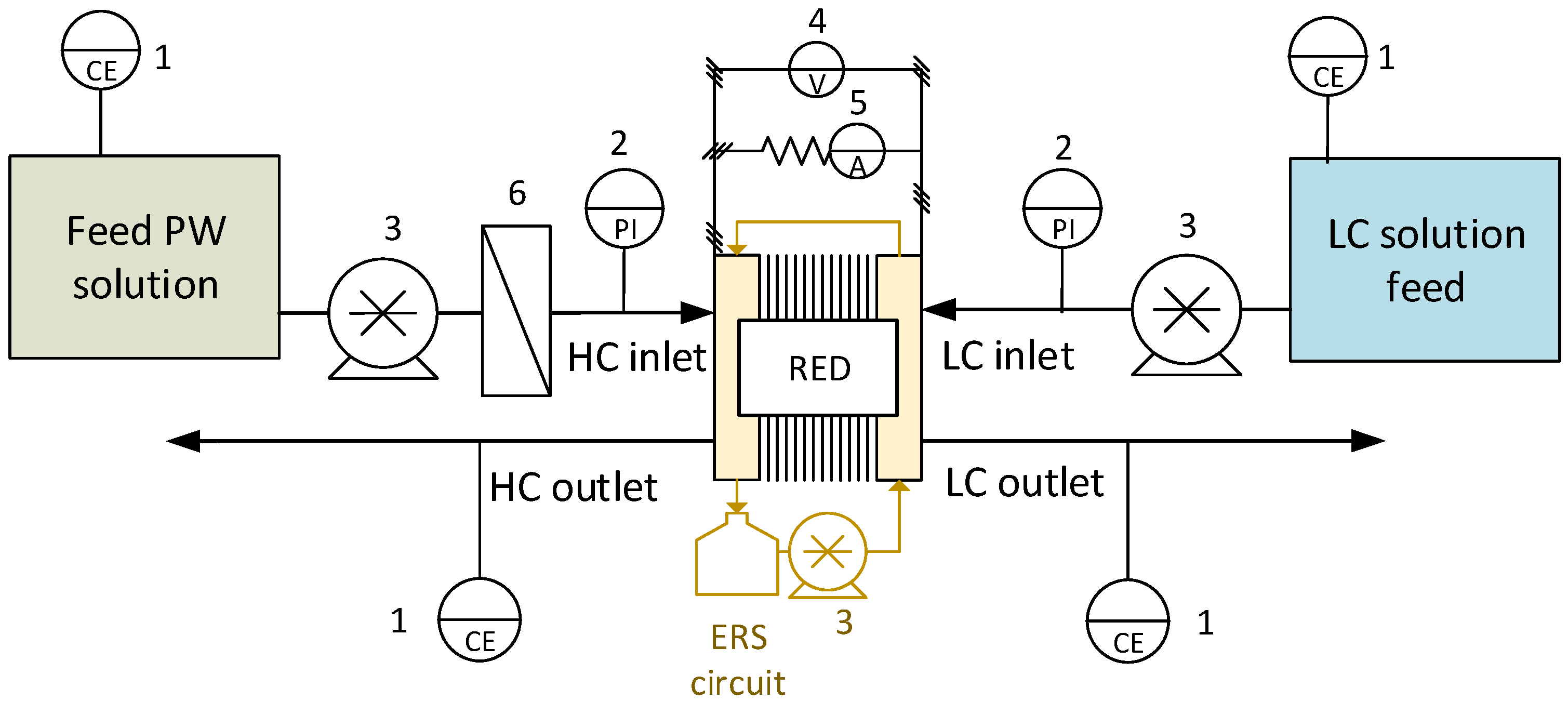
An RED unit is made of several repetitive units called cell pairs, consisting of two channels and two IEMs, i.e., an anion exchange membrane (AEM) and a cation exchange membrane (CEM). Spacers are interposed between the membranes to generate the two channels where a concentrate solution (or high-concentration solution, HC) and a dilute solution (or low-concentration solution, LC) are alternatively fed. The salinity gradient across each IEM generates a potential difference, leading to an ionic flux between the two adjacent solutions. At the two ends of the stack, electrode compartments are placed. In these compartments, an electrode rinse solution (ERS), containing redox couples, is continuously recirculated, allowing the conversion of the ionic flux into electric current when an external load is connected to the RED unit. Between each electrode compartment and the cell pairs, an end-membrane is interposed.

2.1. Feed Solutions

Two different real wastewaters (PW1 and PW2), from two different oil industrial wells located in southern Europe, were studied as the feed solution in an RED unit. After an in-place oil separation treatment, they were used as high-concentration feed (HC). The main features of these solutions are reported in Table 2 and Table 3. In particular, PW1 contains a larger amount of ions and organic compounds (i.e., total dissolved solid, TDS = 74.4 g/L and total organic carbon, TOC = 368.3 ± 3.6 mg/L) than PW2 (i.e., TDS = 46.3 g/L and TOC of 109.9 ± 2.9 mg/L).
To analyse the influence of the use of real solutions on the RED unit performance, the two real HC solutions were also artificially reproduced by preparing synthetic solutions that comprised NaCl-water only, mimicking the conductivity of the real solutions (see Table 3).
All tests were performed by considering as low-concentration (LC) feed solution, a synthetic solution of pure NaCl, and demineralized water with a concentration of 0.7 g/L and a conductivity of 1.49 mS/cm. This concentration value was selected to mimic the typical concentration of process water available in the relevant oil extraction industries. Recrystallized NaCl solid from Volterra (Italy) with a purity of 99.8% and demineralized water with a conductivity lower than 10 μS/cm were used to prepare all the artificial solutions.

2.2. Experimental Set-Up

Two different units were used for the experimental campaign (Stack 1 and Stack 2), both composed of 10 cell pairs with an active membrane area of 10 × 10 cm2. In Stack 1, polyamide woven spacers 300 μm thick, with a silicone gasket (provided by Redstack, Sneek, The Netherlands), were interposed between the ionic exchange membranes. In Stack 2, overlapped spacers in polyamide with a thickness of 270 μm (provided by Deukum, Frickenhausen, Germany) were adopted. The end plates of both units are made of PMMA and two Ru-Ir oxides coated titanium electrodes were located there.
The adopted ion exchange membranes were provided by Fujifilm (Tilburg, The Netherlands) (Type 10 AEM and CEM) while the two end-membranes by Fumatech (Bietigheim-Bissingen, Germany) (Fumasep FKS-50). The main properties, from the technical datasheet provided by the companies, of the membranes are reported in Table 4.
The membranes, once cut and drilled, were placed for 24 h in a 35 g/L NaCl solution for conditioning. Polypropylene cartridge filters (Water Hi-Tech from Italy Water, Carini, Italy) with decreasing pore sizes (10, 5, and 1 μm) were used to filtrate the two PWs before feeding them to the RED unit.
Two peristaltic pumps (Leadfluid WT/600/S, He Bei Sheng, China) were used to feed the solutions into the stack with a co-current arrangement. Another peristaltic pump (Seko Kronos 50, Rieti, Italy) was used to recirculate the ERS. The two solutions, stored in a tank of 20 L, were fed at a flow rate of about 90 mL/min in Stack 1 and about 80 mL/min in Stack 2. These flow rate values correspond to an inlet velocity of about 0.5 cm/s within the channels (empty channel without spacers). Typically, feed velocities of 1 cm/s are used in laboratory tests for RED systems [50]. However, the use of real wastewaters may produce significant pumping losses due to fouling and bio-fouling phenomena. An inlet channel velocity of 0.5 cm/s was considered a good compromise between keeping “power losses as low as possible” and worsening the concentration polarization effects.
The electrode rinse solution (ERS) was prepared by dissolving 0.1 moles of K3[Fe(CN)6] (Sigma Aldrich, St. Louis, MO, USA, >99%), 0.1 moles of K4[Fe(CN)6]∙3H2O (Sigma Aldrich, >99%), and 0.58 moles of NaCl (99.8% Sigma Aldrich) in a liter of demineralized water. NaCl was used in the ERS as supporting electrolyte, in such a quantity as to replicate the total concentration of ions corresponding to the average concentration of the two feed solutions (HC and LC).
Alkaline (pH = 12) and acid (pH = 3) solutions for the chemical cleaning were prepared with demineralized water and sodium hydroxide (solid NaOH > 99%, Sigma Aldrich) and hydrochloric acid (HCl 37%, Sigma Aldrich), respectively.
The ion concentration was determined by ion chromatography analysis, carried out with a Metrohm 822 Compact Plus IC equipped with the cation-exchange Metrosep C4 and the anion-exchange Metrosep A Supp 5 columns (Herisau, Switzerland). Pressure transducers (VEGA-14, Assago, Italy), placed at the inlet of the two channels, were used to monitor the pressure drops inside the stack. To measure the conductivity and pH of the solutions, a portable WTW Profiline pH-Cond 3320 conductivity/pH-meter, equipped with a TetraCon 325 conductivity cell and a SenTix 41pH electrode (from Xylem, Weilheim in Oberbayern, Germany) was used. An electronic load (BK8540, B&K Precision, Yorba Linda, CA, USA), connected to the RED electrodes, was used to close the external electric circuit. Two multi-meters (Fluke 175 True RMS, Everett, WA, USA) were used for measuring the voltage and current. Two 0.5 W UV lamps (Aquael UV, Suwalki, Poland) were used in each LC solution reservoir during some tests, along with a recirculation submersible pump (Prodac Pump 200, Cittadella, Italy) working at 100 L/h.
The main specifications of the test-rig instruments are reported in Table 5.

2.3. Experimental Procedures

The performance of the system was investigated firstly with short-time spot tests (a), and subsequently, in continuous operations, with three different long-run tests with a time duration of up to 26 days (b).
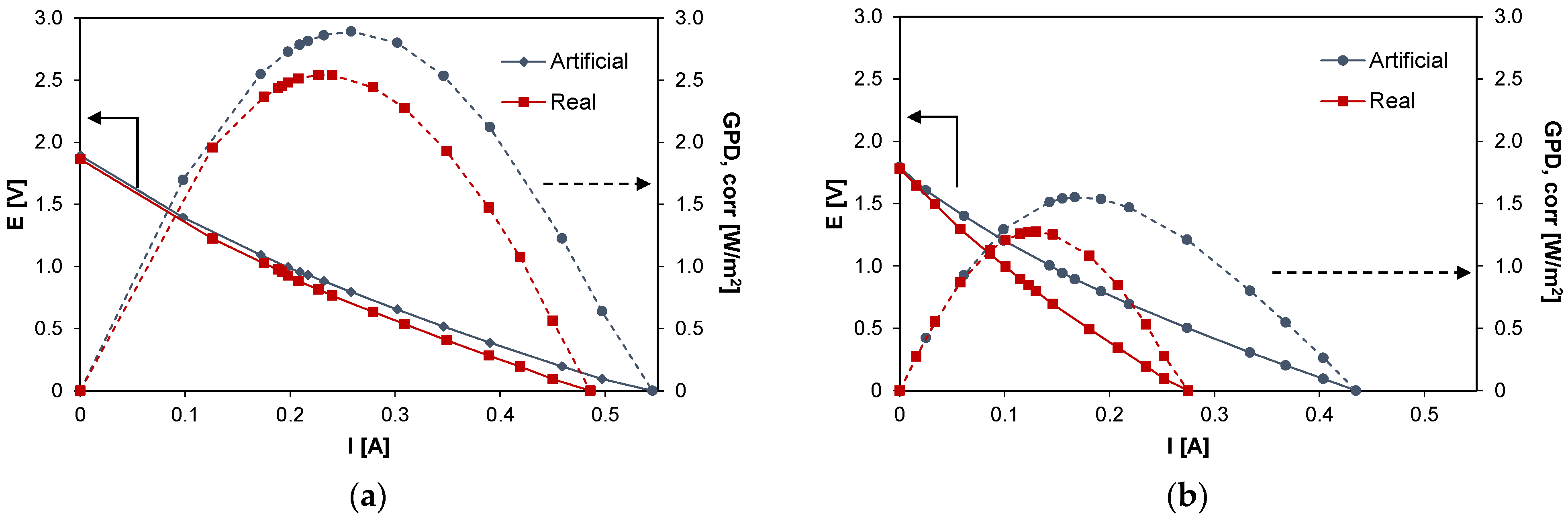
(a) In the spot tests, the RED unit operated in once-through mode with fresh solutions continuously fed to the system. To highlight the impact of using real PWs, the performance of the system was first evaluated by feeding the stack with the artificial solutions and, secondly, with the real HC solutions. To this aim, the conventional procedure used to characterize the RED unit performance in terms of current/voltage and power density/voltage curves [16,20,23] was adopted. The RED unit was connected to the external electronic load, which stepwise varies the value of the external resistance from the open-circuit (OC) to short-circuit (SC) condition, measuring both the stack voltage (E) and current (I). The open circuit voltage (OCV) is defined as the electrical voltage of the stack in the OC condition. The electrical resistance of the stack (Rstack) is inferred from the slop of the E vs. I linear trend. The product of E times I gives the generated gross power of the system (Pgross, see Equation (1)). The gross power density (GPD, Equation (2)) curve is obtained by normalizing each value of the power for the number of cell pairs (N) and the active membrane area (A):
P g r o s s = E · I ,
G P D = P g r o s s N · A ,
The maximum gross power density value of the GPD vs. E curve corresponds to the condition in which EOCV/2, i.e., when the stack internal resistance Rstack is almost equal to the external load. The net power density value (NPD, Equation (3)) includes the pumping losses directly related to the pressure drops inside the stack:
N P D = P d , g r o s s P p u m p N · A ,
where Ppump is the total power required for the pumping of the two streams inside the RED unit.
Ppump is calculated by Equation (4):
P p u m p = P L C Q L C + P H C Q H C ,
where P H C and P L C are the overall pressure drops in the RED unit along the concentrated (HC) and diluted (LC) channels, respectively, while Q H C and Q L C are the corresponding volumetric flow rates.
The power density values evaluated using a small lab-scale unit constituted by few cell pairs are strongly influenced by the blank resistance (Rblank). The latter is the contribution to Rstack given by the electrical resistance of the electrode compartments (more specifically, given by the (i) electrode rinse solution, (ii) electrodes, and (iii) one end-membrane). When stacks with a high number of cell pairs (larger than 100) are considered, the influence of Rblank might be neglected with respect to the resistance of the cell pairs, which provides the greatest contribution to Rstack. The Rblank can be evaluated through the physical measurement of the electrical resistance of the unit assembled with only one end membrane and fed with only the electrode rinse solution. An Rblank value of about 0.27 Ω was found in our system. Thus, to evaluate the power density of scaled-up units, the so-called corrected (gross) power density (GPD,corr) is evaluated by subtracting the blank resistance from the resistance of the stack [22]. Similarly, the net correct power density (NPD,corr) can be easily calculated from the GPD,corr (see Equation (3)) by subtracting the pumping power density.
The average permselectivity of the IEMs is evaluated by comparing the experimental OCV with the theoretical OCV according to Equation (5):
α = O C V r e a l O C V t h e o r e t i c a l ,
In particular, the theoretical OCV is evaluated by using the Nernst equation [51,52]. A schematic representation of the once-through configuration of the test rig is reported in Figure 1.
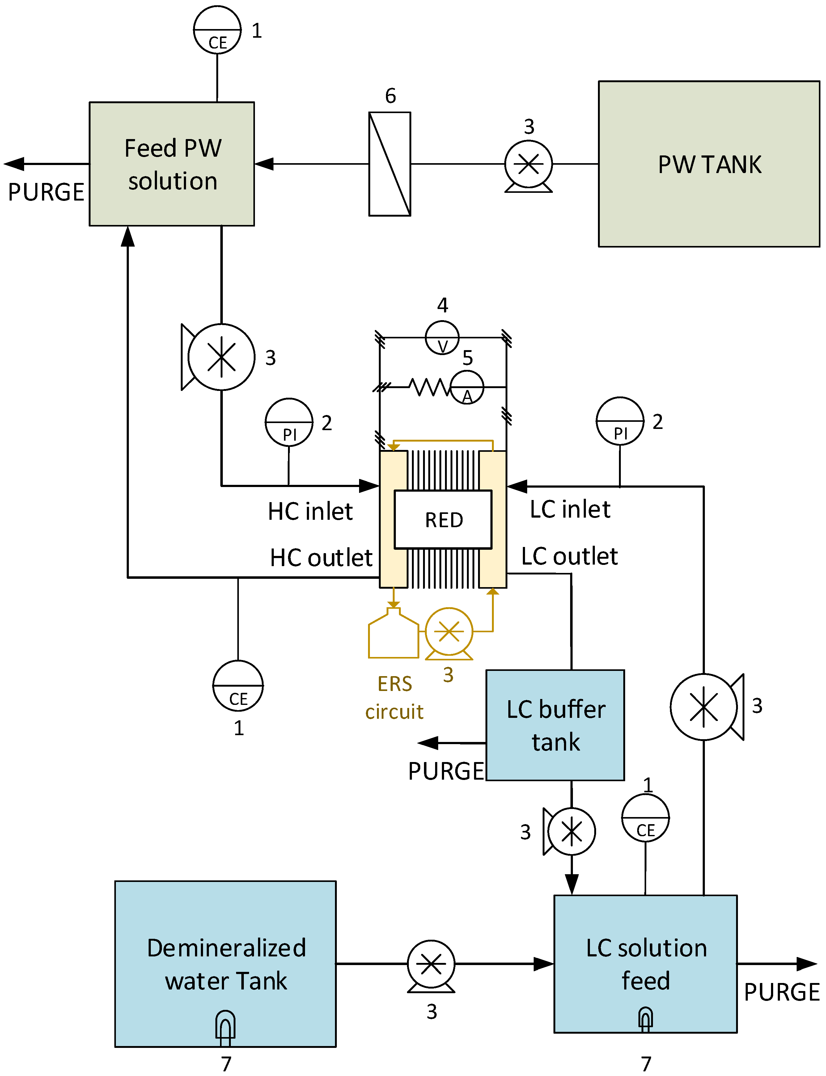
(b) The long-run tests were performed using PW1 and PW2 as HC and the artificial NaCl solution as LC arranged in steady concentration mode. In this configuration, the concentrations of the feed solutions are kept at a fixed constant value by considering a feed and bleed arrangement, i.e., a partial recycle system, with a ratio of purged solution. In other words, an equal amount of solution is continuously purged and made-up. A transition period (start-up) is required by the system in the first days of the test to reach the steady condition. During this period, the PW in the feed reservoir leads the concentration to the fixed value while the membranes are adapting to the new operating conditions. The purpose of working in the steady concentration mode is to simulate in a lab-scale unit, a portion of a hypothetical industrial system constantly operating with the same concentration of the feed solutions. The equivalent NaCl concentrations of the HC in the different tests performed at a steady concentration were kept constant at 25.7 g/L during the long-run I, at 50.3 g/L during the long-run II, and at 29.8 g/L during the long-run III. Similarly, in all the tests, the LC solution was maintained at a fixed concentration, i.e., 0.7 g/L, using a similar feed and bleed arrangement, which reduced the consumption of demineralized water.
During the long-run operations, the RED unit was connected to a fixed external load. The value of the external electrical resistance was chosen to operate the system around the maximum power density condition. During the experiments, the performance of the system was tested using the spot test procedure (a), evaluating the temporal variation of the power density, the stack resistance, and the pressure drops. This guaranteed monitoring of the conditions of the IEMs exposed to fouling issues. A schematic representation of the test rig is reported in Figure 2.
In the present work, three different long-run tests were performed to study the performance of RED units fed by real PWs.
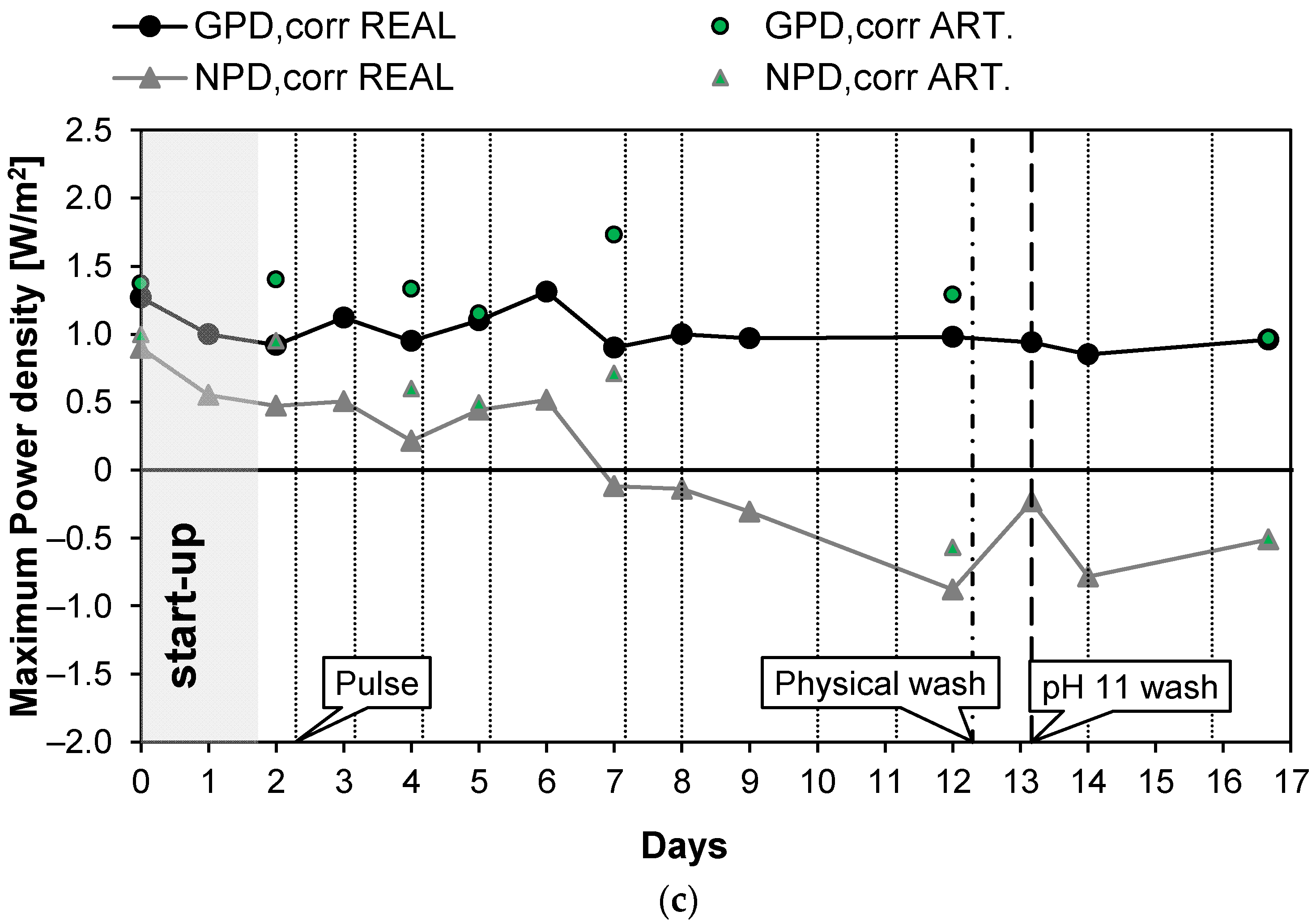
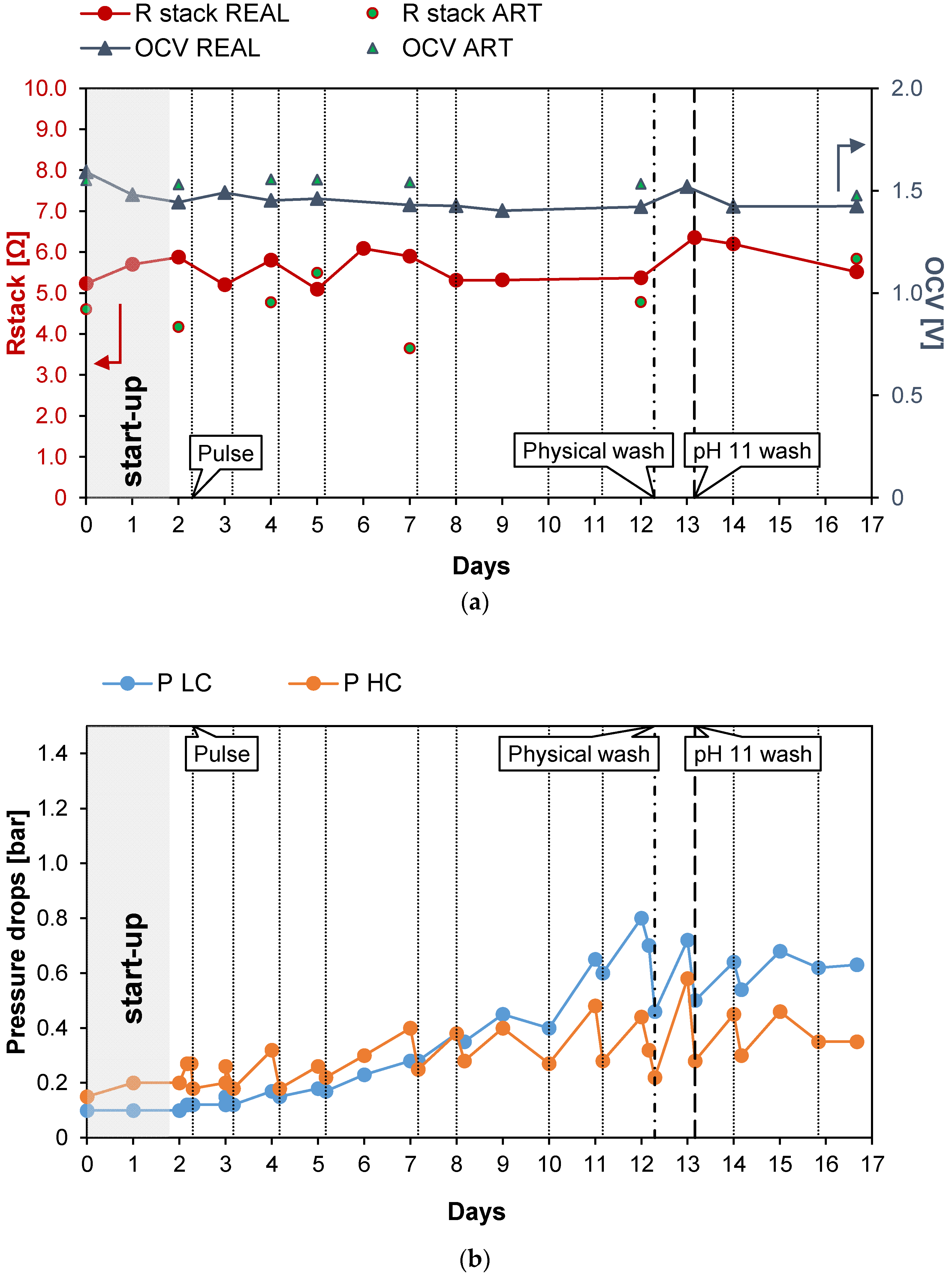
  • In the long-run test I, the RED unit (Stack 1) was operated in steady concentration mode; thus, both PW1 and the artificial LC are posed in a feed and bleed fashion. The concentration of PW1 was fixed at an equivalent concentration of about 25.7 g/L. For this test, Stack 1 operated for about 17 days and to counteract the fouling phenomena, some anti-fouling actions were performed. When pressure drops were too high, the flow rates of the two-feed solutions were impulsively increased from the normal value (i.e., 80 mL/min) to 1600 mL/min, for about 2 s. In other words, a “pulse” in the flow rates was carried out to aid the removal of substances clogging the channels out from the unit. This operation was repeated 3–6 times, until a reduction in the pressure drops was observed. Moreover, physical or chemical washes were adopted. When the pulses started to not be effective, a physical counter washing was carried out by switching the inlet and the outlet and increasing the flow feed flow rate at about 800 mL/min for 10 min, thus allowing the cleaning of channels in the opposite direction with respect to the normal operative condition. After the washing, the stack was set to the standard inlet/outlet configuration. The chemical washing of the system was carried out by stopping the normal operation and feeding, for a few minutes, NaOH solutions (pH = 11) in the channels. The washing operation was completed when no variation between the inlet and the outlet values of the pH was obtained, and then, a washing of the channels with demineralized water was performed before restarting the test with the nominal feeds.
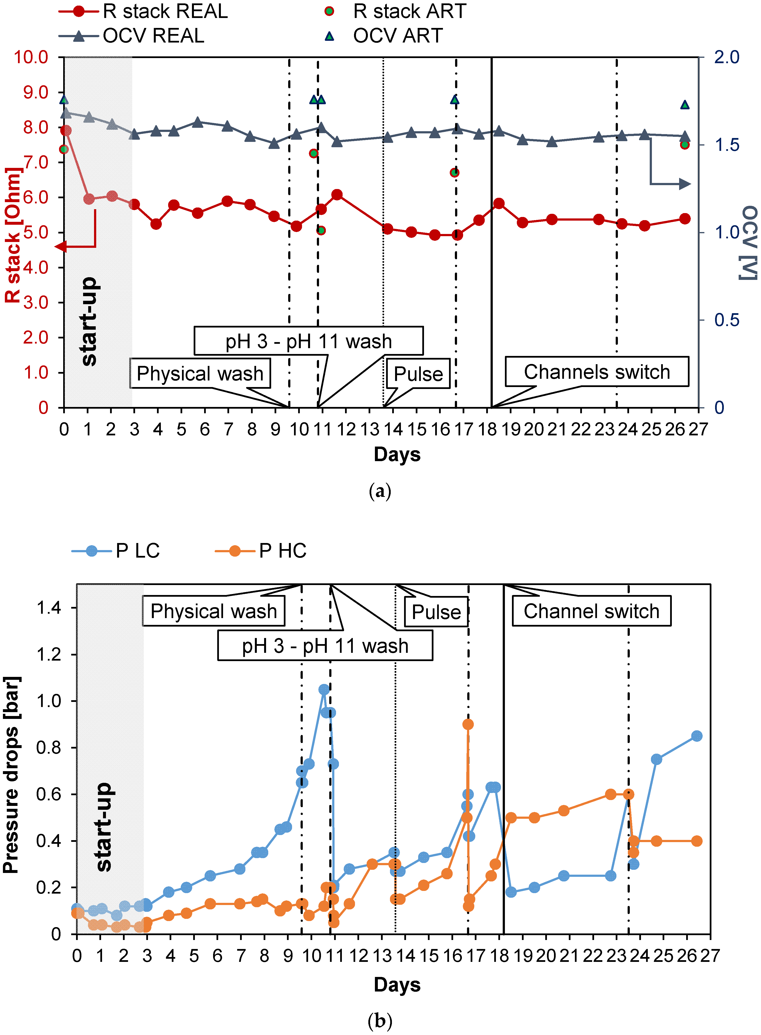
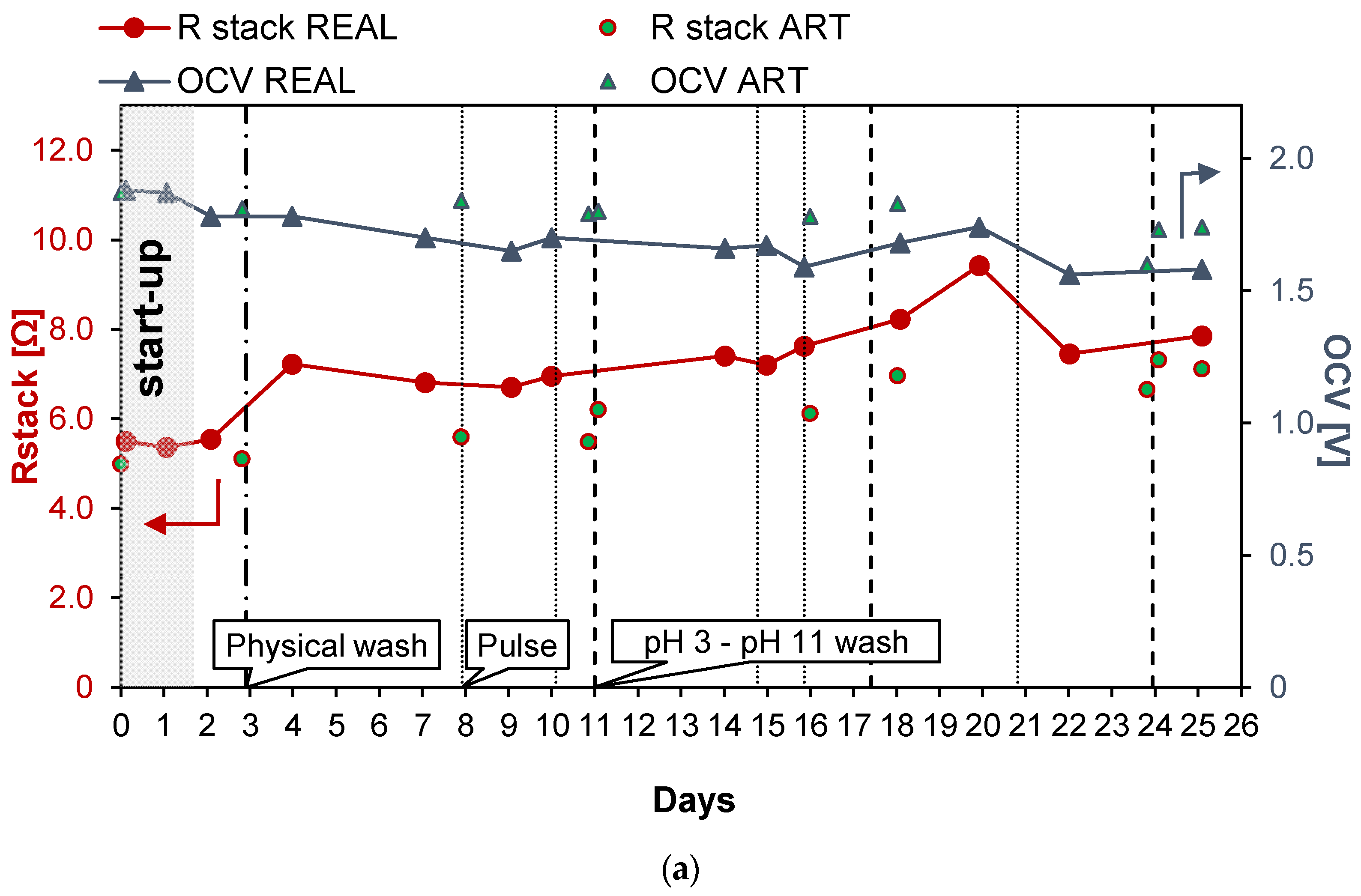
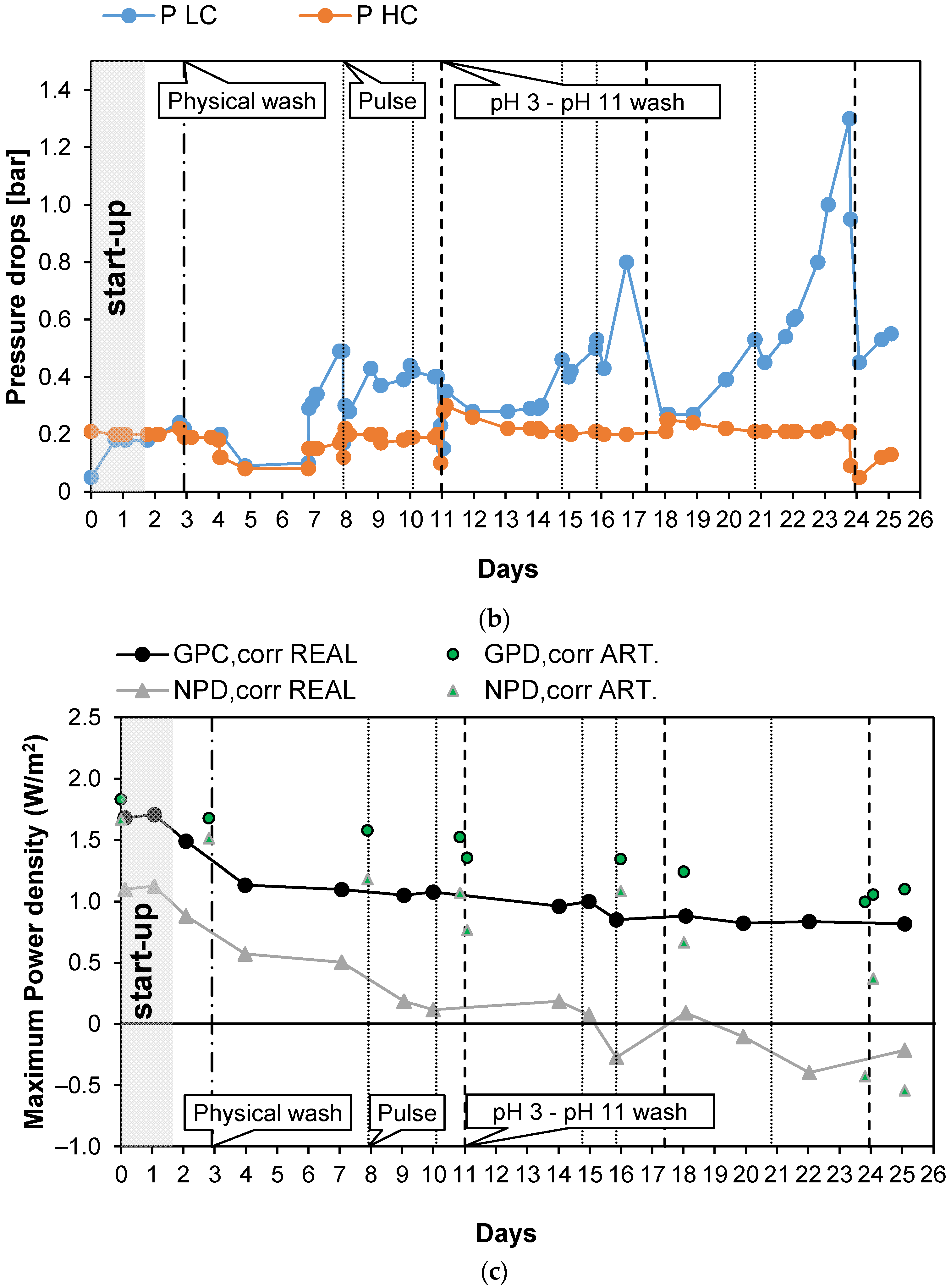
  • In the long-run test II, Stack 2 was operated for 25 days as in the previous long run but with the concentration of the inlet PW1 fixed at an equivalent concentration of about 50.3 g/L. The chemical washing of the system was carried out using both acid and alkaline solutions (solutions of HCl, pH = 3, and NaOH, pH = 11, respectively). In addition to the previous antifouling strategies, a UV lamp was installed in the LC tank to avoid bacteria and algae proliferation.
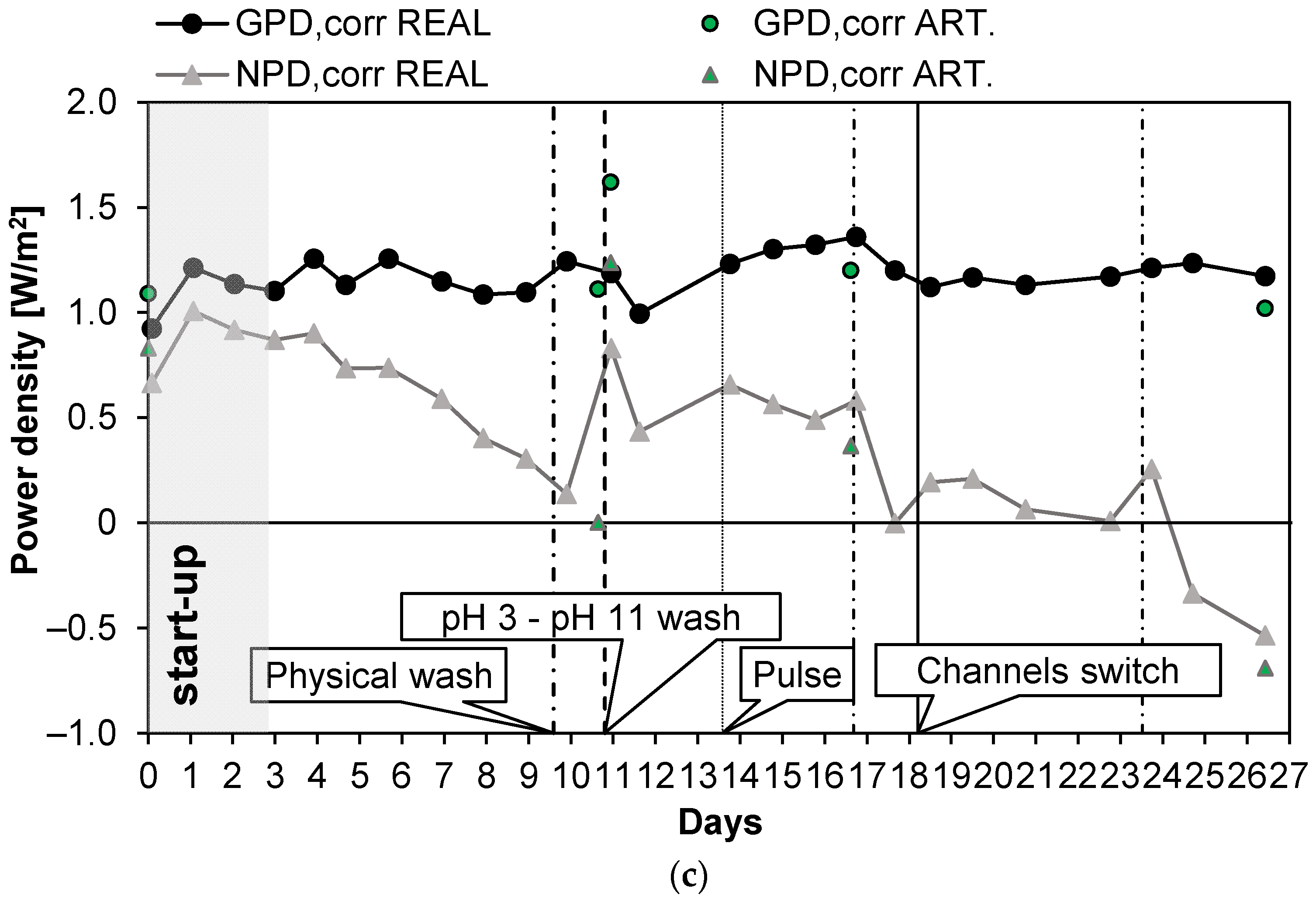
  • In the long-run test III, Stack 1 was operated for 26 days using PW2 at an equivalent concentration of 29.8 g/L and the artificial LC as feeding solutions both in the feed and bleed configuration. In addition to the previous antifouling strategies, the channel switch was also considered. To this aim, the HC was sent in the LC channels, and vice versa, to modify the habitat of any bacteria colony eventually formed inside the channels.
A summary of the main conditions and antifouling strategies adopted in the three long-run tests are reported in Table 6.

3. Results and Discussion

3.1. Preliminary Tests

This section reports the results of the preliminary tests performed on the system. Figure 3 shows the typical curves for RED experiments, i.e., current vs. voltage and current vs. corrected power density, for the case of the artificial (blue symbols) and the real HC solutions (red symbols). In particular, Figure 3a reports the results for the case of PW1 while Figure 3b reports the case of PW2. The performance of the system is affected by the type (artificial/real) of HC solution fed to the system: for the case of PW1, GPD,corr decreased from 2.89 W/m2 with artificial solutions to 2.54 W/m2 with real PW, with a loss of ~12%, while in the case of PW2, the effect was slightly more marked and the corrected power density decreased from 1.55 to 1.29 W/m2 (−17%).
Despite the difference between the two feed concentrations, the results show very close OCV values, i.e., 1.86 V for the case of PW1 and 1.78 V for the case of PW2. The theoretical Nernst OCVs evaluated considering the equivalent NaCl concentration for the PW1 and PW2 are equal to 2.09 and 1.85 V, respectively. Thus, in the case of the real HC solutions, the corresponding IEMs average permselectivities are equal to αreal (PW1) = 0.89 and αreal (PW2) = 0.96 while in the case of artificial solutions, these values are equal to αart (PW1) = 0.90 and αart (PW2) = 0.97. Slight permselectivity variations were observed shifting from natural to artificial HC solutions, thus suggesting that the salts contained in the real HC solutions, other than NaCl, have little influence on the average permselectivity of the IEMs.
As it can be seen in Figure 3a, E vs. I curves for the real and artificial PW1 solutions have a very similar trend: the stack resistance of the system fed with PW1 is equal to about 3.6 Ω for the real case, 8% greater than the value relevant to the corresponding artificial solution case (3.3 Ω). A more marked difference was obtained for PW2 (Figure 3b), in which a stack resistance value of 6.4 Ω was obtained with the natural solution and a value of 3.9 Ω (−40%) with the artificial solution.
This preliminary test confirms the negative effect of minority ions and impurities dissolved in the feed solutions. For this reason, the performances of the RED unit with real PW were tested for a long period to monitor how the fouling could affect the membranes’ operation.

3.2. Long-Run Tests

The first long-run test was performed with the conductivity of the real PW1 kept constant at a value of 42.2 mS/cm (25.7 g/L of NaCl) thanks to the feed and bleed lay-out (see Figure 2). In the first 2 days of the long-run test, the system drove itself to a steady state (start-up): the IEMs adapted to the real feed and the conductivity of the solutions stabilized at its nominal values. Subsequently, the test proceeded for another 15 days continuously, and spot tests were carried out both with real PW and artificial solutions. During the investigation, to counteract the clogging of channels, pulses were applied to the feed flow rates. Moreover, since the effect of the pulses was limited, a physical washing was performed on day 12 and a chemical wash with an alkaline solution on day 13. The time evolution of the investigated parameters measured during the test is reported in Figure 4. In particular, Figure 4a shows the behavior of Rstack and OCV. The OCV measured with the natural feed after the start-up phase is quite constant and had an average value of about 1.44 V. The OCV gives information about the permselectivity of the IEMs (see Equation (5)), which is practically constant during all of the test. Conversely, Rstack increased from the starting value of 5.88 to 6.35 Ω during the 13th day (+7%) and then decreased again to 5.52 Ω during the last day, probably thanks to the positive effect of the alkaline wash performed on the 13th day. Figure 4b shows the trend of the pressure drops in the HC and LC channels. As expected, due to the physical fouling, the pressure drops in both channels continuously increased from the start to the end of the test. In particular, the HC pressure drops grew from the initial value of 0.15 to 0.35 bar while the pressure drops in the dilute channels increased from the initial value of 0.1 to 0.63 bar recorded in the last day of the test. The trend of the pressure drops is not linear but shows a saw-tooth profile with marked picks, especially in the LC channels. This behavior is caused by the application of anti-fouling strategies that promote the reduction of the pressure losses in both channels. Both physical and chemical washes reduced the increase in the pressure drops. In particular, the LC pressure drop decreased from 0.7 to 0.44 bar (−0.26 bar) with the physical wash operated on the 12th day while the chemical washes, executed on the 13th day, resulted in a reduction in the pressure drops from 0.72 to 0.5 bar (−0.22 bar). The physical fouling was more prominent for the LC channel, in which bacteria easily proliferate, causing clogging in the LC channels of the stack. On the contrary, the high salinity of the PW prevented bacteria proliferation in the HC channels, justifying the lower pressure drops observed. Figure 4c shows the trend of the maximum gross and net corrected power densities measured during the 17 days of the test. After the start-up, as a result of the OCV and Rstack behavior, the correct power density was quite constant around the initial value of 0.92 W/m2. In the case of the artificial solution spot tests, the value was slightly higher, with an average value of about 1.18 W/m2. The increase in the pressure drops, and the consequent increase in the pumping power, led to a decrease in the net power density from the starting values of 0.9 and 1.00 W/m2 for the case of natural and artificial feed respectively, which reached negative values after six days.
Figure 5 shows the results obtained during long-run test II, in which the conductivity of the PW1 was kept constant at 74.6 mS/cm (about 50.3 g/L of NaCl) and Stack 2 was used. To reduce the bacteria proliferation, UV lamps were installed in the LC tank. With respect to the previous long run, the duration of the test was increased to 25 days of continuous operation. Moreover, in this case, a start-up of 2 days was required to stabilize the feed and the stack conditions. Figure 5a shows the trend of the OCV, which decreased very slowly since the start of the test to the last day. In particular, in the case of real PW, the OCV decreased from 1.78 (day 2) to 1.58 V (day 25), with a loss of about −11% while in the case of artificial HC, OCV decreased from 1.87 to 1.74 V (about −7%). Conversely, Rstack increased during the test from the minimum initial value of 5.55 Ω on day 2 to a value of 7.85 Ω (+29%), recorded on the last day of the tests.
As shown in Figure 5b, during the long-run test II, the pressure drops in the LC channels were kept at lower values than in long-run I thanks to the antifouling strategies adopted and particularly to the additional installation of UV lamps. Three chemical washes were executed during the test, carried out using both an acid (at pH = 3) and an alkaline solution (at pH = 11), and showed an immediate positive effect on the LC channels’ pressure drops.
The benefits obtained from both the UV lamps and chemical washes confirm that the main cause of the increase in the pressure drops observed during the long run test I was the proliferation of bacteria, especially in the LC solution. This is not surprising because LC solution is stored in a tank, where bacteria and algae growth are strongly promoted.
The adoption of a higher value of the inlet PW concentration than in the previous test led to higher values of the gross power density, which from the initial value of 1.49 W/m2, during day 2, decreased to 0.82 W/m2 after 23 days of continuous operations (see Figure 5c). The increase in the gross power density together with the maintenance of a low value of the pressure drops resulted in a positive value of the net power density up to the 15th day of the tests.
Long-run III (see Figure 6) was carried out with PW2. The conductivity of the feed was kept at a constant value of 47 mS/cm (about 29.8 g/L of NaCl) and Stack 1 was employed. Moreover, in this case, UV lamps were installed in the tanks of the LC stream circuit. The first 3 days were employed for the start-up of the system. The test was almost 27 days long, and during these days, the number of anti-fouling actions was quite low. The OCV was almost constant (Figure 6a) at a value of 1.55 V and Rstack, after the start-up phase, similarly, assumed values of around 5.5 Ω, with a maximum of 6.1 Ω on the 12th day (an increase of 10%). As a consequence, the gross power density (Figure 6c) was almost constant along all the long-run test, with an average value of 1.18 W/m2. After day 10, the pressure drops of the LC channels increased excessively, leading to a large reduction in the net power density to 0.14 W/m2 and the need for a chemical wash. The effect of the latter was highlighted by the quick increase in the net power density from a value of 0.14 to 0.83 W/m2. On the 18th day, another important increase in the pressure drops and a consequent large reduction in the net power density were observed; thus, a channel switch was executed to observe the effect of increasing salinity on the bacteria colonies that grew in the LC channel. The pressure drops (Figure 6b) in the LC channel decreased by 70%, restoring a value of 0.18 bar, which is close to the initial one (i.e., 0.1 bar). The net power density increased to 0.19 W/m2, equal to the 22% of the initial net power density. After this last action, the net power density assumed low but positive values until the 24th day. The system response demonstrates that the switching of the channels could also have a positive effect on the control of the pressure drops. On day 24, a new physical wash was necessary to reduce the pressure drops, but a limited effect on time was observed after this.

4. Conclusions

This work represents, to the author’s knowledge, the first work in which real produced waters were used as feeds in RED units to produce energy. Three long-run tests were carried out with two kinds of produced waters, originating from two different sites. The membrane’s properties (electrical resistance and permselectivity) seemed to be poorly affected by the presence of pollutants and minority species in the produced waters. Interestingly, the results showed that it is possible to produce energy from produced waters, and valorize such industrial wastewater using in situ operations via RED systems. The maximum power density obtained was about 2.5 W/m2, which is perfectly comparable to values reported in the literature for streams with similar salinity gradients and, overall, similar to those obtained with artificial solutions. Indeed, when membranes and channels are still clean, no important losses of efficiency due to the pollutants contained in the feed were observed. The membranes, after an initial period of conditioning, presented an electrical resistance that increased slightly over time. The main issue is represented by the fouling, in particular, channel clogging, which is probably due to bacteria growing in the channels of the RED unit and in the dilute solution circuit. The use of anti-fouling actions, such as the use of chemical washes and physical counter washes, allowed the RED unit to be continuously operated for about 25 days. However, negative values of net the power density occurred after a few days of operation. As a result, the coupling of UV lamps and acid-alkaline washes ensured positive power density values until the 18th day. In particular, it was observed that the UV lamps prevented bacterial proliferation in the LC solution and the consequent clogging of the RED unit channels by the bacteria colonies. In fact, the problem of bacteria growth mainly occurred in the LC solution, since the high concentration of salt in the brine depressed the activity of the bacteria. Moreover, the long storage time of solutions in the laboratory promoted the growth of bacteria. This is expected to be less dramatic in industrial processes, where continuous solutions are fed to the system. Benefits may come from a continuous switching of the solutions (e.g., once per day or per hour). Moreover, other additional methods could be implemented, for example, the use of periodic ED pulses that prevent the adsorption of pollutants on the membranes’ surface, thus keeping the stack resistance constant.
Overall, there is still room for further improvements and anti-fouling strategies still need to be carefully integrated and tuned. On the other hand, the preliminary collected results are quite promising and suggest that the use of saline waste streams in RED systems may lead to new scenarios for the application of such systems in industries and treatment plants, enlarging the potential of the salinity gradient power.

Author Contributions

Conceptualization, A.C. (Adrea Cipollina), A.C. (Alessandro Cosenza) and A.T.; methodology, A.C. (Adrea Cipollina), A.C. (Alessandro Cosenza), A.T., G.C. and F.G.; formal analysis, F.G. and S.R.; investigation, A.C. (Alessandro Cosenza) and G.C.; data curation, A.T., F.G., G.C. and S.R.; writing—original draft preparation, A.C. (Alessandro Cosenza); writing—review and editing, A.T., F.G. and S.R.; visualization, A.C. (Adrea Cipollina), F.G. and S.R.; supervision, A.T. and A.C. (Adrea Cipollina); project administration, A.C. (Adrea Cipollina) and G.M.; funding acquisition, A.T. and G.M. All authors have read and agreed to the published version of the manuscript.

Funding

This research received no external funding.

Institutional Review Board Statement

Not applicable.

Informed Consent Statement

Not applicable.

Data Availability Statement

Not applicable.

Conflicts of Interest

The authors declare no conflict of interest. The funders had no role in the design of the study; in the collection, analyses, or interpretation of data; in the writing of the manuscript, or in the decision to publish the results.

Acronyms

AEMAnionic Exchange Membrane
BTEXbenzene, toluene, ethylbenzene and xylene
CEMCationic Exchange Membrane
CODChemical Oxygen Demand
ERSelectrode rinse solution
HChigh concentration
IEMionic exchange membrane
LClow concentration
MBRmembrane bio-reactor
OCopen circuit
PROpressure retarded osmosis
PWproduced water
REDreverse electrodialysis
SCshort circuit
SGPsalinity gradient power
TDStotal dissolved solids
TOCtotal organic carbon
TSStotal suspended solids
UVultra-violet
WORwater oil ratio
αpermselectivity

Nomenclature

A m 2 active membrane area
E V stack voltage
GPD W m 2 gross gower density
GPD,corr W m 2 gross correct power density
I A stack current
N number of cell pairs
NPD W m 2 net power density
NPD,corr W m 2 net correct power density
OCV V open circuit voltage
Pgross W gross power
Q m 3 s flow rate
Rblank Ω blank electrical resistance
Rstack Ω stack electrical resistance
Ppump W m 2 pumping power
P Pa pressure drops

References

  1. Neff, J.; Lee, K.; Deblois, E. Produced Water: Overview of Composition, Fates, and Effects. In Produced Water: Environmental Risks and Advances in Mitigation Technologies; Elsevier: New York, NY, USA, 2011; Volume 90, pp. 1–21. [Google Scholar]
  2. Dudek, M.; Vik, E.A.; Aanesen, S.V.; Øye, G. Colloid chemistry and experimental techniques for understanding fundamental behaviour of produced water in oil and gas production. Adv. Colloid Interface Sci. 2020, 276, 102105. [Google Scholar] [CrossRef] [PubMed]
  3. Veil, J.A.; Puder, M.G.; Elcock, D.; Redweik, R.J., Jr. A White Paper Describing Produced Water from Production of Crude Oil, Natural Gas, and Coal Bed Methane; Office of Scientific and Technical Information: Washington, DC, USA, 2004.
  4. Al-Ghouti, M.A.; Al-Kaabi, M.A.; Ashfaq, M.Y.; Da’Na, D.A. Produced water characteristics, treatment and reuse: A review. J. Water Process Eng. 2019, 28, 222–239. [Google Scholar] [CrossRef]
  5. Shahlol, O.M.A.; Isawi, H.; El-Malky, M.G.; Al-Aassar, A.E.-H.M.; Elzwi, A. Assessment of the Physico-Chemical Properties of Produced Water from Sarir Oil Field in Sirt Basin, Libya. J. Environ. Sci. 2019, 47, 1–19. [Google Scholar] [CrossRef]
  6. Samuel, O.; Othman, M.H.D.; Kamaludin, R.; Sinsamphanh, O.; Abdullah, H.; Puteh, M.H.; Kurniawan, T.A.; Li, T.; Ismail, A.F.; Rahman, M.A.; et al. Oilfield-Produced Water Treatment Using Conventional and Membrane-Based Technologies for Beneficial Reuse: A Critical Review. J. Environ. Manag. 2022, 308, 114556. [Google Scholar] [CrossRef]
  7. Collins, A.G. Geochemistry of Oilfield Waters; Elsevier: New York, NY, USA, 1975; p. 413. [Google Scholar]
  8. Zoungrana, A.; Çakmakci, M. From non-renewable energy to renewable by harvesting salinity gradient power by reverse electrodialysis: A review. Int. J. Energy Res. 2020, 45, 3495–3522. [Google Scholar] [CrossRef]
  9. Fakhru’L-Razi, A.; Pendashteh, A.; Abdullah, L.C.; Biak, D.R.A.; Madaeni, S.S.; Abidin, Z.Z. Review of technologies for oil and gas produced water treatment. J. Hazard. Mater. 2009, 170, 530–551. [Google Scholar] [CrossRef] [PubMed]
  10. Jiménez, S.; Micó, M.M.; Arnaldos, M.; Medina, F.; Contreras, S. State of the art of produced water treatment. Chemosphere 2018, 192, 186–208. [Google Scholar] [CrossRef]
  11. Amoatey, P.; Izady, A.; Al-Maktoumi, A.; Chen, M.; Al-Harthy, I.; Al-Jabri, K.; Msagati, T.A.; Nkambule, T.T.; Baawain, M.S. A critical review of environmental and public health impacts from the activities of evaporation ponds. Sci. Total Environ. 2021, 796, 149065. [Google Scholar] [CrossRef]
  12. Wenzlick, M.; Siefert, N. Techno-economic analysis of converting oil & gas produced water into valuable resources. Desalination 2020, 481, 114381. [Google Scholar] [CrossRef]
  13. Seip, A.; Safari, S.; Pickup, D.M.; Chadwick, A.V.; Ramos, S.; Velasco, C.A.; Cerrato, J.M.; Alessi, D.S. Lithium recovery from hydraulic fracturing flowback and produced water using a selective ion exchange sorbent. Chem. Eng. J. 2021, 426, 130713. [Google Scholar] [CrossRef]
  14. Mondal, S.; Wickramasinghe, S. Photo-induced graft polymerization of N-isopropyl acrylamide on thin film composite membrane: Produced water treatment and antifouling properties. Sep. Purif. Technol. 2012, 90, 231–238. [Google Scholar] [CrossRef]
  15. Nie, H.; Nie, M.; Diwu, Z.; Wang, L.; Yan, H.; Lin, Y.; Zhang, B.; Wang, Y. Biological treatment of high salinity and low pH produced water in oilfield with immobilized cells of P. aeruginosa NY3 in a pilot-scale. J. Hazard. Mater. 2020, 381, 121232. [Google Scholar] [CrossRef]
  16. Veerman, J.; Saakes, M.; Metz, S.; Harmsen, G. Reverse electrodialysis: Performance of a stack with 50 cells on the mixing of sea and river water. J. Membr. Sci. 2009, 327, 136–144. [Google Scholar] [CrossRef] [Green Version]
  17. Giacalone, F.; Papapetrou, M.; Kosmadakis, G.; Tamburini, A.; Micale, G.; Cipollina, A. Application of reverse electrodialysis to site-specific types of saline solutions: A techno-economic assessment. Energy 2019, 181, 532–547. [Google Scholar] [CrossRef]
  18. Helfer, F.; Lemckert, C.; Anissimov, Y.G. Osmotic power with Pressure Retarded Osmosis: Theory, performance and trends—A review. J. Membr. Sci. 2014, 453, 337–358. [Google Scholar] [CrossRef] [Green Version]
  19. Ju, J.; Choi, Y.; Lee, S.; Jeong, N. Comparison of fouling characteristics between reverse electrodialysis (RED) and pressure retarded osmosis (PRO). Desalination 2020, 497, 114648. [Google Scholar] [CrossRef]
  20. Veerman, J.; Saakes, M.; Metz, S.J.; Harmsen, G.J. Electrical Power from Sea and River Water by Reverse Electrodialysis: A First Step from the Laboratory to a Real Power Plant. Environ. Sci. Technol. 2010, 44, 9207–9212. [Google Scholar] [CrossRef]
  21. Nam, J.-Y.; Hwang, K.-S.; Kim, H.-C.; Jeong, H.; Kim, H.; Jwa, E.; Yang, S.C.; Choi, J.; Kim, C.-S.; Han, J.-H.; et al. Assessing the behavior of the feed-water constituents of a pilot-scale 1000-cell-pair reverse electrodialysis with seawater and municipal wastewater effluent. Water Res. 2019, 148, 261–271. [Google Scholar] [CrossRef]
  22. Bevacqua, M.; Carubia, A.; Cipollina, A.; Tamburini, A.; Tedesco, M.; Micale, G. Performance of a RED system with ammonium hydrogen carbonate solutions. Desalin. Water Treat. 2016, 57, 23007–23018. [Google Scholar] [CrossRef] [Green Version]
  23. Giacalone, F.; Vassallo, F.; Scargiali, F.; Tamburini, A.; Cipollina, A.; Micale, G. The first operating thermolytic reverse electrodialysis heat engine. J. Membr. Sci. 2019, 595, 117522. [Google Scholar] [CrossRef]
  24. Volpin, F.; Woo, Y.C.; Kim, H.; Freguia, S.; Jeong, N.; Choi, J.-S.; Cho, J.; Phuntsho, S.; Shon, H.K. Energy recovery through reverse electrodialysis: Harnessing the salinity gradient from the flushing of human urine. Water Res. 2020, 186, 116320. [Google Scholar] [CrossRef]
  25. Yamada, Y.; Sowa, K.; Kitazumi, Y.; Shirai, O. Improvement in the Power Output of a Reverse Electrodialysis System by the Addition of Poly(sodium 4-styrenesulfonate). Electrochemistry 2021, 89, 467–471. [Google Scholar] [CrossRef]
  26. Vermaas, D.A.; Saakes, M.; Nijmeijer, K. Doubled Power Density from Salinity Gradients at Reduced Intermembrane Distance. Environ. Sci. Technol. 2011, 45, 7089–7095. [Google Scholar] [CrossRef]
  27. Mehdizadeh, S.; Yasukawa, M.; Abo, T.; Kuno, M.; Noguchi, Y.; Higa, M. The Effect of Feed Solution Temperature on the Power Output Performance of a Pilot-Scale Reverse Electrodialysis (RED) System with Different Intermediate Distance. Membranes 2019, 9, 73. [Google Scholar] [CrossRef] [PubMed] [Green Version]
  28. Kingsbury, R.S.; Liu, F.; Zhu, S.; Boggs, C.; Armstrong, M.D.; Call, D.F.; Coronell, O. Impact of natural organic matter and inorganic solutes on energy recovery from five real salinity gradients using reverse electrodialysis. J. Membr. Sci. 2017, 541, 621–632. [Google Scholar] [CrossRef]
  29. Bodner, E.; Saakes, M.; Sleutels, T.; Buisman, C.J.N.; Hamelers, H.V.M. The RED Fouling Monitor: A novel tool for fouling analysis. J. Membr. Sci. 2018, 570–571, 294–302. [Google Scholar] [CrossRef]
  30. Vermaas, D.A.; Kunteng, D.; Veerman, J.; Saakes, M.; Nijmeijer, K. Periodic Feedwater Reversal and Air Sparging As Anti-fouling Strategies in Reverse Electrodialysis. Environ. Sci. Technol. 2014, 48, 3065–3073. [Google Scholar] [CrossRef] [PubMed]
  31. Moreno, J.; de Hart, N.; Saakes, M.; Nijmeijer, K. CO2 saturated water as two-phase flow for fouling control in reverse electrodialysis. Water Res. 2017, 125, 23–31. [Google Scholar] [CrossRef]
  32. Chon, K.; Jeong, N.; Rho, H.; Nam, J.-Y.; Jwa, E.; Cho, J. Fouling characteristics of dissolved organic matter in fresh water and seawater compartments of reverse electrodialysis under natural water conditions. Desalination 2020, 496, 114478. [Google Scholar] [CrossRef]
  33. Vermaas, D.A.; Kunteng, D.; Saakes, M.; Nijmeijer, K. Fouling in reverse electrodialysis under natural conditions. Water Res. 2012, 47, 1289–1298. [Google Scholar] [CrossRef]
  34. Avci, A.H.; Tufa, R.A.; Fontananova, E.; Di Profio, G.; Curcio, E. Reverse Electrodialysis for energy production from natural river water and seawater. Energy 2018, 165, 512–521. [Google Scholar] [CrossRef]
  35. Vital, B.; Torres, E.V.; Sleutels, T.; Gagliano, M.C.; Saakes, M.; Hamelers, H.V.M. Fouling Fractionation in Reverse Electro-dialysis with Natural Feed Waters Demonstrates Dual Media Rapid Filtration as an Effective Pre-Treatment for Fresh Water. Desalination 2021, 518, 115277. [Google Scholar] [CrossRef]
  36. Hossen, E.H.; Gobetz, Z.E.; Kingsbury, R.S.; Liu, F.; Palko, H.C.; Dubbs, L.L.; Coronell, O.; Call, D.F. Temporal variation of power production via reverse electrodialysis using coastal North Carolina waters and its correlation to temperature and conductivity. Desalination 2020, 491, 114562. [Google Scholar] [CrossRef]
  37. Gómez-Coma, L.; Ortiz-Martínez, V.M.; Fallanza, M.; Ortiz, A.; Ibañez, R.; Ortiz, I. Blue Energy for Sustainable Water Rec-lamation in WWTPs. J. Water Process Eng. 2020, 33, 101020. [Google Scholar] [CrossRef]
  38. Mehdizadeh, S.; Yasukawa, M.; Suzuki, T.; Higa, M. Reverse electrodialysis for power generation using seawater/municipal wastewater: Effect of coagulation pretreatment. Desalination 2020, 481, 114356. [Google Scholar] [CrossRef]
  39. Tedesco, M.; Scalici, C.; Vaccari, D.; Cipollina, A.; Tamburini, A.; Micale, G. Performance of the first reverse electrodialysis pilot plant for power production from saline waters and concentrated brines. J. Membr. Sci. 2016, 500, 33–45. [Google Scholar] [CrossRef] [Green Version]
  40. Tedesco, M.; Cipollina, A.; Tamburini, A.; Micale, G. Towards 1 kW power production in a reverse electrodialysis pilot plant with saline waters and concentrated brines. J. Membr. Sci. 2017, 522, 226–236. [Google Scholar] [CrossRef] [Green Version]
  41. Mehdizadeh, S.; Yasukawa, M.; Kuno, M.; Kawabata, Y.; Higa, M. Evaluation of energy harvesting from discharged solutions in a salt production plant by reverse electrodialysis (RED). Desalination 2019, 467, 95–102. [Google Scholar] [CrossRef]
  42. Budi, S.H.; Susanto, H. Hermawan The potential recovery energy of SWD (sea water desalination) by SGP (salinity gradient power). J. Phys. Conf. Ser. 2021, 1858, 012078. [Google Scholar] [CrossRef]
  43. Yasukawa, M.; Mehdizadeh, S.; Sakurada, T.; Abo, T.; Kuno, M.; Higa, M. Power generation performance of a bench-scale reverse electrodialysis stack using wastewater discharged from sewage treatment and seawater reverse osmosis. Desalination 2020, 491, 114449. [Google Scholar] [CrossRef]
  44. Avci, A.H.; Sarkar, P.; Tufa, R.A.; Messana, D.; Argurio, P.; Fontananova, E.; Di Profio, G.; Curcio, E. Effect of Mg2+ ions on energy generation by Reverse Electrodialysis. J. Membr. Sci. 2016, 520, 499–506. [Google Scholar] [CrossRef]
  45. Rijnaarts, T.; Huerta, E.; Van Baak, W.W.; Nijmeijer, D.K. Effect of Divalent Cations on RED Performance and Cation Exchange Membrane Selection to Enhance Power Densities. Environ. Sci. Technol. 2017, 51, 13028–13035. [Google Scholar] [CrossRef]
  46. Guo, Z.; Ji, Z.; Zhang, Y.; Yang, F.; Liu, J.; Zhao, Y.; Yuan, J. Effect of Ions (K+, Mg2+, Ca2+ and SO42−) and Temperature on Energy Generation Performance of Reverse Electrodialysis Stack. Electrochim. Acta 2018, 290, 282–290. [Google Scholar] [CrossRef]
  47. Moreno, J.; Díez, V.; Saakes, M.; Nijmeijer, K. Mitigation of the effects of multivalent ion transport in reverse electrodialysis. J. Membr. Sci. 2018, 550, 155–162. [Google Scholar] [CrossRef]
  48. Di Salvo, J.L.; Cosenza, A.; Tamburini, A.; Micale, G.; Cipollina, A. Long-run operation of a reverse electrodialysis system fed with wastewaters. J. Environ. Manag. 2018, 217, 871–887. [Google Scholar] [CrossRef]
  49. Abbas, T.; Al-furaiji, M. Use of Reverse Electrodialysis to Harvest Salinity Gradient Energy from Oilfield Produced Water. Pollution 2021, 7, 943–957. [Google Scholar] [CrossRef]
  50. Tedesco, M.; Brauns, E.; Cipollina, A.; Micale, G.; Modica, P.; Russo, G.; Helsen, J. Reverse electrodialysis with saline waters and concentrated brines: A laboratory investigation towards technology scale-up. J. Membr. Sci. 2015, 492, 9–20. [Google Scholar] [CrossRef] [Green Version]
  51. Tedesco, M.; Hamelers, H.V.M.; Biesheuvel, P.M. Nernst-Planck Transport Theory for (Reverse) Electrodialysis: I. Effect of Co-Ion Transport through the Membranes Channel. J. Memb. Sci. 2016, 510, 370–381. [Google Scholar] [CrossRef]
  52. Długołęcki, P.; Nymeijer, K.; Metz, S.J.; Wessling, M. Current status of ion exchange membranes for power generation from salinity gradients. J. Membr. Sci. 2008, 319, 214–222. [Google Scholar] [CrossRef]
Figure 1. Once-through mode set-up, used for the preliminary and periodical tests. The numbers indicate: 1—Conductivity meter; 2—Pressure indicator; 3—Peristaltic pump; 4—Voltage indicator; 5—Current indicator; 6—Cartridge filter.
Energies 15 04177 g001
Figure 2. Schematic layout of the lab-scale system used for the long-run tests. The numbers indicate: 1—Conductivity-meter; 2—Pressure indicator; 3—Peristaltic pump; 4—Voltage indicator; 5—Current indicator; 6—Cartridge filter; 7—UV lamps (used in long-run II and III only).
Energies 15 04177 g002
Figure 3. Voltage (E) vs. current (I) and gross power density (GPD,corr) vs. current (I) curves with artificial (in blue) and real solutions (in red) for the case of (a) PW1 and (b) PW2.
Energies 15 04177 g003
Figure 4. Time evolution of OCV and Rstack (a), pressure drops in the LC and HC channels (b), and maximum GPD,corr and maximum NPD,corr (c) for long-run I.
Energies 15 04177 g004aEnergies 15 04177 g004b
Figure 5. Time evolution of OCV and Rstack (a), pressure drops in the LC and HC channels (b), and maximum GPD,corr and maximum NPD,corr (c) for the long-run II.
Energies 15 04177 g005aEnergies 15 04177 g005b
Figure 6. Time evolution of OCV and Rstack (a), pressure drops in the LC and HC channels (b), and maximum GPD,corr and maximum NPD,corr (c) for Long-run III.
Energies 15 04177 g006aEnergies 15 04177 g006b
Table 1. Main properties of produced waters.
PropertyRange
Density [kg/m3]1014–1140
pH4.3–10
Surface Tension [mN/m]43–78
Total Organic Carbon [mg/L]0–1500
Total Dissolved Solids [g/L]0–300
Total organic acids [mg/L]0.001–10,000
COD [mg/L]1220–2600
Total BTEX [mg/L]0.73–24.1
Saturated hydrocarbons [mg/L]17–30
Table 2. Main ion composition of the real produced waters investigated.
IonsPW1 [mg/L]PW2 [mg/L]
Na+23,08013,500
Ca2+19802950
Mg2+670.0480.0
K+107090.00
B3+109.817.30
Li+9.4001.100
Rb+2.6600.303
Cl45,70029,090
HCO31400200.0
SO42−420.0<1.000
Other ions<1.000<1.000
TDS74,44246,329
Table 3. Physical-chemical properties of the real produced waters.
PropertyPW1PW2
pH7.578.05
Total Organic Carbon (TOC) [mg/L]368.3 ± 3.6109.9 ± 2.9
Conductivity [mS/cm]97.172.4
Equivalent NaCl concentration [g/L]67.848.5
Total Suspended Solids (TSS) [mg/L]270 ± 40292 ± 60
Table 4. Main properties of the IEMs used for the experimental campaign.
PropertyAEM Type 10CEM Type 10Fumasep FKS-50
Thickness (dry) [μm]12513545–55
Electrical resistance [Ω cm2]1.7 a2.0 a1.8–2.5 c
Permselectivity [%]95 b99 b97–99 d
a Measured at 2 M NaCl. b Measured at 0.05−0.5 M KCl. c Measured in 0.5 M NaCl at T = 25 °C, in a standard measuring cell (through-plane). d Measured at 0.1/0.5 mol/kg KCl at T = 25 °C determined from the membrane potential measurement in a concentration cell.
Table 5. Main specifications of the test-rig instruments.
InstrumentSpecification
PumpsFeed solutions: Leadfluid WT/600/S. Range: 3–6000 mL/min.
ERS: Seko Kronos 50. Range: 2–25,000 mL/h.
External loadB&K Precision BK8540. Range: 0.1–10 Ω, resolution 0.001 Ω; range: 10–99 Ω, resolution 0.01 Ω; range: 100–4000 Ω, resolution 1 Ω. Accuracy: ±(1% + 0.8% FS).
Pressure TransducersVEGA-14. Range: 0–2.5 bar. Accuracy: ±0.3% FS.
Multi-metersFLUKE 175 True RMS. Range: 0.1 mV–1000 V and 0.01 mA–10 A. Accuracy: V DC ± (0.15% + 2 counts) A DC ± (1.0% + 3 counts).
Conductivity meterWTW ProfiLine pH/Cond 3320. Range: 0.000–1000 mS/cm. Accuracy: ±0.5% FS.
UV lampsAquael UV, 0.5 W, with recirculation submersible pump: Prodac Pump 200, range 100 a 300 L/h.
Table 6. Summary of the conditions used for the three long-run tests.
Long-RunPWEquivalent NaCl Concentration HC [g/L]Anti-Fouling ActionsStackDuration [Days]
I125.7Pulse, physical wash, and chemical wash (pH 11)117
II150.3Pulse, physical wash, chemical wash (pH 3, pH 11), UV lamps225
III229.8Pulse, physical wash, chemical wash (pH 3, pH 11), UV lamps, channel switch126
Publisher’s Note: MDPI stays neutral with regard to jurisdictional claims in published maps and institutional affiliations.

