Abstract
This research aimed to introduce a comprehensive mathematical modeling approach based on the maximization of the power coefficient (Cp) to obtain the regulation in pitch angle and tip speed ratio (TSP), taking into account the detailed power losses at the different stages of the power train of the wind turbine. The model is used to track the optimal power coefficient of the wind turbine power train, considering both direct (without gearbox) and indirect (with gearbox) drive configurations. The result of the direct driveline was validated with a 100 W horizontal-axis wind turbine experimental system. The model estimated the optimal value of Cp at 0.48 for a pitch angle of 0 degrees and a TSR of 8.1, which could be obtained at a wind speed of around 11.2 m/s. The results also revealed that, within the lower wind regime, windage, hysteresis, and eddy current losses dominated, while during higher wind regimes, the copper, stray load, and insulator gate bipolar transistor (IGBT) losses gained high values. The developed model was applied to a 20 kW indirect drive wind turbine installed in Gwadar city in Pakistan. Compared with the direct coupling, the optimal value of Cp was obtained at a higher value of the pitch angle (1.7 degrees) and a lower value of TSR (around 6) due to the significant impact of the gear and copper losses in an indirect drivetrain.
1. Introduction
1.1. Background and Literature Review
In recent decades, the depletion of fossil fuel sources and increased power demand have created the space for green energies to support conventional power generation in energy sectors. Wind energy offers sustainable and renewable energy solutions to meet energy demands and mitigate climate change. This has driven researchers to investigate the optimal design of renewable energy systems that include wind turbines [1,2], as well as propose advanced control systems for the optimal power tracking of both wind and PV energy [3]. However, the maximum energy generation of a wind turbine cannot be achieved without optimal range regulation of the power coefficient and loss minimization of the turbine [4,5,6].
The extraction of maximum power from wind turbine systems is significantly reliant on a dimensionless quantity, namely, the power coefficient (Cp). Considering wind turbine operational dynamics, the role of two regimes of variable wind speed is critical for both the extraction of maximum power and the safety of the wind turbine. For example, the wind regime under the nominal wind speed limit requires maximum power extraction, as the tip speed ratio is a function of wind speed and the pitch angle of the turbine blades. In the same way, the wind regime above the nominal value of wind speed presents some concerns about the safety of the turbine blades, gearbox, and electric machine. This issue can only be handled by regulating the value of Cp during the regime between nominal and cutout limits of wind speed.
Many maximum-power-tracking and optimization methods were proposed for regulating the wind turbine mechanical structure’s positions and parameters, such as yaw, tip speed ratio, pitch angle, angular speed, and torque [7,8,9,10,11,12,13,14]. In the last few decades, several studies were carried out on power coefficient optimization and expanded through several theoretical, ideal analyses, maximum tracking points, and optimization based on different methodologies and perspectives [15,16,17]. Peng et al. developed a novel composite model with a higher calculation accuracy of the wind turbine power coefficient and flapping moment coefficient by taking into account the NREL 5 MW windmill [5]. In their study, the analysis of effective parameters of a wind system, such as the role of the tip speed ratio on the axial induction factor, pitch angle, and aerodynamic torque coefficient, and studies of trust force coefficient were comprehensively carried out. It was concluded that under uncertain wind situations, the vertical axis wind turbines rotate to generate aerodynamic power associated with their characteristic curves based on the power coefficient and tip speed ratio, which is a function of the angular speed of the turbine and wind velocity. In another study, Pongpak et al. developed a real-time maximum power generation of vertical-axis wind turbines, taking into account the characteristics curves of turbine power coefficient through fuzzy pulse width modulation electric load regulation. In their work, the rotational speed extracting the maximum power was firmly managed via the angular speed of the wind turbine based on the optimal value of tip speed ratio for each value of wind speed using the fuzzy logic PWM load regulation technique. It was concluded that across one day, the energy produced by the proposed model under varying wind speed conditions was higher than a wind turbine that works under uncontrolled open-field conditions [18]. The value of the performance coefficient = 0.9981 indicates the two vertical axis wind turbines were identical for cross verification, taking into account the period from 0–24 h. Dongran Song et al. developed a sequential global optimization problem for the maximum power extraction of a wind turbine based on a single-objective and non-linear function by taking into account constraints such as the weighting factor and electric torque variation of the generator [19]. Liangyue Jia et al. presented a reinforcement learning-based method for efficiently searching the optimal value of the blade twist angle distribution (TAD), which is a function of the power coefficient. The basic concept of RL-TAD is to learn the TAD searching policy through an agent and salvage this agent to search for the optimal TAD under changing wind regimes based on genetic algorithm methodology. The empirical results concluded that the power coefficient is better and converges to a value of TAD 3 to 5 times faster than the genetic algorithm method in the offline stage [20].
1.2. Research Gap and Originality Highlights
Previous studies mainly focused on addressing the power coefficient tracking subjected to boundary conditions related to wind speed and the aerodynamic train of the wind turbine, such as the blade design and pitch angle or TSR. However, few studies have addressed the impact of the optimal power coefficient on the load regulation of the power train and power loss reduction of wind turbines.
Therefore, following the previous studies, this research aimed to introduce a comprehensive mathematical modeling approach based on the maximization of the power coefficient to obtain regulation of the pitch angle, power coefficient, angular speed, and torque, taking into account the detailed power losses at the different stages of the power train of the wind turbine system. Toward this aim, two coupling configurations of wind turbine drivetrains were considered, including direct and indirect coupling with the generator. The direct-coupling configuration had the prominent edge over indirect coupling as the power drop due to friction and lubrication viscosity in the gear stage could be saved on a small scale, and a low-speed wind turbine consisted of at least a four-pole electric machine for operation. The model results were validated with the experimental wind turbine emulator, which consisted of a baseline 100 W horizontal wind turbine that was directly coupled with a four-pole permanent magnet synchronous generator (PMSG). The proposed study of optimal Cp was further enhanced by applying the developed model in a real case scenario wherein the baseline turbine capacity was a 20 kW indirect drive wind turbine consisting of a gearbox that was installed in Gwadar city in Pakistan. Moreover, the developed model is applicable to all kinds of wind turbines, regardless of the amount of power and place of use.
The rest of the paper is organized as follows: In Section 2, the mathematical model of the wind turbine power coefficient, along with the constraints and types of losses, are explained, considering all unavoidable stages of the turbine power train. Section 3 covers the results and discussions of Cp maximization and minimum power loss optimization models. The final section concludes the paper based on the findings of this study.
2. Model Development
The power coefficient of a turbine is tightly managed at the optimal value of the tip speed ratio determined by the aerodynamic angular speed and linear wind velocity in order to yield the maximum aerodynamic work in a wide range of wind regimes. The maximization model of the power coefficient can then be expressed as follows:
subject to:
where is the power coefficient; , , , , , and are the aerodynamic power coefficients; is the value of the TSR; is the pitch angle of the blades, and is the TSR of the turbine. , , , and are the coefficients of the TSR; is the mechanical power under nominal wind speed and is a function of torque and angular speed of the turbine in W [21]; v is the wind speed in m/s; is the cut-in wind speed required to acerate the turbine shaft; is the nominal value of the wind speed in m/s; is the cut-out wind speed, which is considered a feasible value for the operation; is the angular speed of the turbine in rad/s; is the torque of the turbine in N-m; is the nominal value of turbine power in W; and is the effective output power of PMSG. is the total power loss, including all stages and types in W, is the lowest pitch angle in degrees, and is the maximum pitch angle in degrees.
As explained by constraint (3), the wind turbine mechanical drivetrain steps down the high torque belonging to the main shaft of the turbine aperture end to a low torque transfer on the high-speed shaft to meet the electromechanical requirements of the electric source. The size of the wind turbine defines the coupling configuration of the turbine shaft, which is either directly coupled with the generator or indirectly coupled through a gearbox, including a gear train series to ensure the rotational compatibility of the generator in terms of revolution per minute (rpm). Generally, small-scale wind turbines are found directly coupled, while large-size wind turbines require a gear train to interface with an electricity-generating module. The relation of the rotational speed shift from the turbine shaft to the generator shaft in constraint (5) can be estimated as follows:
where n is the rotational speed in revolutions per minute (rpm); denote the gear ratio of each gear; and is the number of gears. The maximum gear ratio is 1:6 [22], and in the case of direct coupling, the ratio will be 1:1. In other words, for a small-size wind turbine directly coupled with a generator, . is the diameter of a turbine (m) and P is the number of poles of a generator. Similarly, the shifting relation of high torque to low torque shaft in constraint (5) can be estimated by using the following formula [23]:
where is the power density (kg/) and r is the radius of the swept area (m).
Constraint (6) indicates that a wind turbine cannot turn 100% of the wind power into effective power. Thus, a significant portion of kinetic energy is distributed in different stages of the turbine, namely, the aerodynamic stage, gearbox stage, electric stage, and inverter stage, in terms of numerous types of power losses, such as swept area loss, gear loss, copper loss, core loss, windage, and IGBT losses. Figure 1 depicts the overall scheme of wind turbines, mapping different types of losses at each stage.
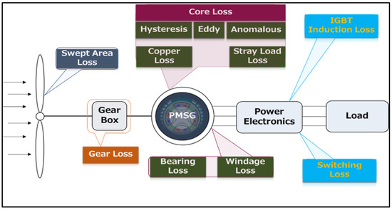
Figure 1.
Wind turbine power train and types of distributed losses.
The total power loss () in constraint (6), which occurs in the different stages of a wind turbine, is calculated as follows:
where is the total power loss distribution in wind turbine; is the swept area loss; is the gearbox loss; is the copper loss in the PMSG; is the core loss, which is further classified into eddy current (, anomalous (, and hysteresis loss ( of an electric machine [24] and is estimated using Equation (16); is the windage loss; is the bearing loss; is the stray load loss; is insulator gate bipolar transistor (IGBT) loss in power electronics devices, such as inverters; and is the forward-switching loss of IGBT.
As depicts a drop in energy during the conversion of aerodynamic kinetic energy into mechanical energy, the difference between the wind power and mechanical power is known as the swept area loss (
where is the wind density in kg/ and r is the turbine radius in m. Furthermore, the gearbox loss can be estimated using the following formula:
where is the gear system efficiency.
PMSG generators require a constant angular speed and torque for magnetization, particularly under the rated wind speed, which can cause frequency and voltage irregularities, and this can be unsafe for the load. Therefore, the power density of a PMSG tends to increase when increasing the rpm of the machine. However, high power is correlated with higher current levels, and major copper and core losses in the stator are related to the current magnitude and operating frequency. The copper loss is associated with the square of the current and the resistance has a positive temperature coefficient, which increases with the rising temperature and can be calculated using
where is the number of phases, is the input current to the PMSG, R is the stator winding resistance, and is the operating voltage of PMSG.
Core losses of the PMSG consist of the eddy current loss (, anomalous loss (, and hysteresis loss ( [25] and can be determined using the nonlinear Steinmetz equation as follows:
where is the frequency, is the hysteresis coefficient, is the eddy current coefficient, is the anomalous coefficient, and is the Steinmetz coefficient [26].
Mechanical losses of the generator consist of the ball bearing loss and windage loss The air friction between the rotor and stator causes a power drop in an electric machine. Windage is a type of air friction loss that occurs due to the air gap between the rotor and stator, and it has a non-linear relationship with the angular speed of the generator. In general, both the windage and bearing losses are minimal in small-scale and low-rotational-speed electric machines, where they can be expressed as [22,27]:
where is the constant associated with the rotor weight, the diameter of the axis, and the rpm, while is a parameter associated with the rotor length and shape. The slots are contained inside the stator windings and power loss due to the proximity effects of slots conductors ( can be estimated as a stray load loss:
In order to obtain the required output voltage and stable frequency, a bi-directional inverter based on power electronic devices, such as IGBT, FET, BJT, and diodes, is used. Even though IGBTs are becoming more efficient, thus far, their power dissipation cannot be ignored; the evaluation of the IGBT and forward-switching losses can be determined with the following approximation equations [27], where the IGBT loss is expressed as
where is the surge current (A), is the IGBT turn-off switching energy (mJ/A), is the IGBT turn-on switching energy (mJ/A), is the carrier frequency, D is the IGBT duty ratio, and a b are the IGBT (on) voltage approximation coefficients. The forward switching losses are calculated using
where is the recovery switching energy (mJ/A), while c and d are the forward voltage approximation coefficients. D is the duty cycle in seconds; is the carrier frequency; and is the surge current, which was assumed to be related to the operating frequency (f), which varied from 0 to 50 Hz, and the current (I), which varied from 0–5 A [27].
3. Results and Discussion
3.1. Estimation of the Optimal Value of the Power Coefficient in a Direct Drive Configuration
The developed model was applied to find the optimal values of the Cp of a 100 W direct-drive wind turbine. The detailed input data used in the model calculation process is given in Table 1.

Table 1.
Input data used in the optimization model.
The power coefficient significantly impacts the transformation of kinetic energy into aerodynamic power. It adopts the power extraction from the swept area under the nominal wind speed. In the case of more robust wind over the turbine’s nominal wind speed, it is necessary to tune the position and speed of the blades to waste excessive energy for the sake of prevention measures. The dynamics of the power train further reduce the unsteady behavior of the wind profile, which requires a variation in the tip speed ratio and pitch angle, both for maximum power extraction and to secure the mechanical structure of the turbine. As a result, the value of Cp varies when the wind velocity increases above the nominal speed. Likewise, the tip speed ratio is a function of the angular speed of the turbine shaft and wind velocity. Therefore, a wind speed above the nominal level causes a steady decrease in Cp.
Figure 2 shows the optimal value of the Cp in the different wind speed regions estimated based on the nonlinear optimization model. To better understand the impact of Cp on the mechanical output power of the wind turbine, the wind speed regions were classified into five regions: no power generation region, acceleration region, active region, optimal region, and finally, power coefficient control region.
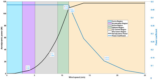
Figure 2.
Variation of the optimal power coefficient with wind speed.
No power generation occurred in the region below the cut-in limit of the wind speed, i.e., a wind speed of under 2.8 m/s; the wind force was unable to accelerate the mechanical structure of the turbine in order to produce electrical power. In this region, the applied kinetic energy was not enough to overwhelm the internal resistance in terms of the losses of the wind turbine. The rated power region was divided into three sub-sections: the acceleration region dealt with above the cut-in and less than a 5.1 m/s wind speed; the active region was where the power exponentially increased with varying wind speeds ranging from 5.1 m/s to 9.7 m/s; and finally, when the wind speed was above 9.7 m/s and was lower than the rated wind speed, i.e., 11.4 m/s, the wind turbine was running in its optimal zone and produced the highest power. In this region, the turbine extracted maximum power from the swept area. Thus, this region was called the maximum-power-coefficient-tracking region. From the no generation region to the optimal region, the optimal values of Cp, pitch angle (), and TSR were estimated to be 0.48, 0°, and 8.1, respectively, in which the turbine rotor gained its rated angular speed corresponding to the wind speed of 11.2 m/s.
In the Cp control region, the mechanical power increases exponentially when the wind speed is observed above the rated speed and below the cut-out speed. Meanwhile, the net mechanical force is proportionally applied to the generator and causes an increase in the rotational speed and torque of the generator. In other words, the rotational speed and torque of the generator exceed their rated limits. As a result, mechanical damage can happen to the generator, such as a bearing fault. However, constraints (7) and (8) in the model were used to level the rated power and rated speed of the turbine by controlling the value of Cp by employing TSR and β control. The maximum value of Cp could be obtained under the nominal limit of the wind regime. When the wind speed increased from the nominal speed, i.e., 11.2 m/s, the value of Cp started to decrease moderately, which is essential for the optimal operation of the wind turbine to ensure the safety of the mechanical and electrical modules of a turbine. The estimated values of Cp based on the TSR and pitch angle shown in Figure 2 were close to those reported in similar works [13,23]. Any value more than the cut-out wind speed, i.e., 26 m/s or more, was critically harmful to the structural damage of the turbine. Since the value of Cp declined to zero at the speed of 25 m/s, as shown in Figure 2, the NLP solver gave an infeasible solution when the speed increased above the cut-out limit. Thus, to prevent any unsafe conditions, the brakes are activated to shut down the turbine and the value of Cp is supposed to be zero at this stage.
Figure 3 shows the variation in the optimal value of Cp with the corresponding optimal values of and TSR.
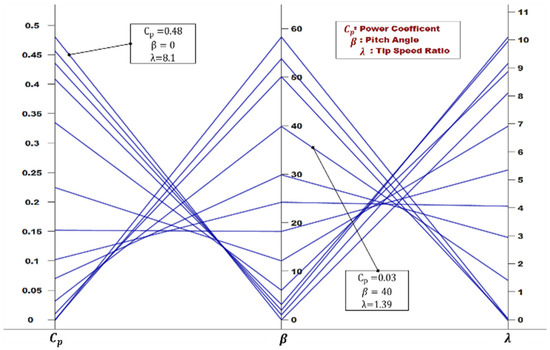
Figure 3.
Variation in the optimal value of the Cp with β and λ.
3.1.1. Power Loss Estimation Based on the Optimal Value of Cp
The distribution of power losses based on the optimal value of Cp is depicted in Figure 4. Based on the results of the model, the optimal value of Cp was estimated to be 0.48; thus, 52% of the total energy was lost in the initial mechanical stage of the turbine’s swept area. Similarly, a considerable amount of power was lost in the PMSG in terms of the copper loss, core loss, stray load loss, bearing loss, and windage loss. Likewise, an amount of power was also dissipated in the bi-directional inverter in order to regulate the operating frequency and voltage. These losses included IGBT power dissipation and switching losses. Windage, hysteresis, and eddy current losses dominated within the lower wind regime, while in higher wind regimes, such as 6.3 m/s to 11.2 m/s, the copper, stray load, and IGBTs losses eventually gained high values in this region. At the wind speed of 5.4 m/s, the copper loss increased due to the higher value of the input current. After the nominal wind speed, around 60% of the power drop consisted of copper and bearing loss, and 40% of the total was distributed to other types, such as anomalous, windage, eddy current, and IGBTs losses, as shown in Figure 4.
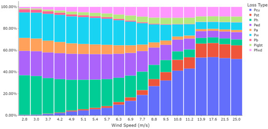
Figure 4.
Distribution of the power losses in different stages of a direct-drive wind turbine.
In other words, the kinetic energy is the function of wind speed and dramatically increases as the wind speed rises steadily. However, the maximum aerodynamic power should not exceed the rated value in order to stabilize and meet the capability of the generator. This can be managed by optimizing the value of the power coefficient, and therefore, the rest of the power is allowed to drop in the swept area first.
3.1.2. Validation of the Model Results with the Experimental System
The result obtained from the model was compared with the measured output power from the experimental system. The experimental system consisted of a 100 W horizontal wind turbine emulator installed at the energy and environmental systems laboratory, Kyushu University, Japan. Figure 5 shows the experimental system consisting of a dynamometer coupled with a 100 W horizontal axis dynamo of PMSG, a 400 W induction motor, and a variable frequency device (VFD) to control the linear frequency and change the angular speed of the induction motor.
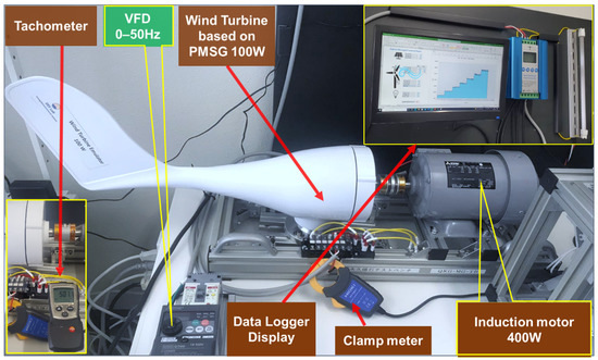
Figure 5.
Wind turbine experimental setup in this study.
Table 2 shows the detailed technical specifications of the experimental setup used in this study.
Table 2.
Technical specifications of the experimental system used in this study.
In order to compare the model results with the experimental system, the input aerodynamic power was artificially generated using the induction motor coupled with the wind turbine. The value of the variable frequency device (VFD) could vary from 0 Hz to 50 Hz, and as a result, the rotational speed also changed in the range of 0 to 1410 rpm. However, theoretically, the value of the rpm was slightly higher than the measured value, where such a difference is called the rpm deviation. To calculate the power that applies to the wind turbine shaft, technical parameters, such as the rotational speed, torque coefficient, rated torque, and machine efficiency, need to be determined. First, the rpm of the wind turbine was measured with the help of a digital tachometer to find the rated torque of the machine, which could be calculated using
where is the rated torque in N-m; is the rated current; is the rated voltage; and η is the machine efficiency, which varies from 10–25% under the nominal range of the linear frequency and the measured rotations per minute (rpm). The actual torque is a function of the rated torque and the torque coefficient, which can be determined based on
where is the actual torque in N-m and is a dimensionless torque coefficient that can be estimated from the torque coefficient curve given by the manufacturer [41], as shown in Figure 6. The value of the torque coefficient of the four-pole 400 W induction motor changed from 0.3 to 0.5 when the frequency was limited between 3 Hz and 6 Hz:
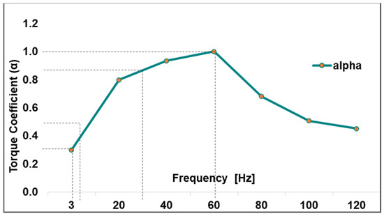
Figure 6.
Torque coefficient curve of the V/F control induction motor used in this study.
In the same way, the response of torque coefficient was observed to be steady and linear from 0.5 to 0.83 within the frequency range of 20–30 Hz:
The range that gave the optimal value of linear frequency, such as 50 Hz, could be extracted from Equation (31). As can be seen in Figure 6, the value of the torque coefficient slightly changed from 0.83 to 1 throughout the full range of the x-axis.
Similarly, in the upper half of the frequency interval, i.e., 60 Hz to 120 Hz, the value of the decreased unsteadily, and it could be calculated using the following nonlinear model equation:
In order to compare the model results with the measured values from the experimental system, the mechanical power (shown in Equation (3) was estimated using the following formula, taking both the measured rpm and actual torque into account:
Applying a different frequency to the induction motor, the output voltage and current of PMSG were measured by the clamp meter connected to the datalogger. The output power measured from the experimental setup was compared with the output power estimated by the model.
The model was tested in two modes: (1) Given a fixed value of Cp at 0.48 [42] and (2) considering the optimal values of Cp obtained from the model using a wide range of wind speeds (shown in Figure 2). As shown in Figure 7, in both modes, the output power estimated by the model showed a similar trend to the experimental system. During the experimental system measurements, the frequency varied from 20–50 Hz with a 5 Hz step difference, and a total of seven measurements were made in this regard. Likewise, the wind speed based on these frequency values was calculated in the range of 4.49–11 m/s. After applying the same wind regime to the mathematical models for both the fixed Cp and dynamic Cp modes, the power at 30 Hz (6.65 m/s of wind speed) was measured at 37.66 W in the experimental system and found to be 41.54 W and 42.71 W in the fixed Cp and dynamic Cp modes, respectively. Similarly, the power at 45 Hz (9.9 m/s) was measured at 83.01 W and was found to be 86.76 W and 90.52 W for the fixed Cp and dynamic Cp modes. Figure 7 shows the power curves based on both model results and measure data from the experimental system. The trends of the three models can be seen in Figure 7, where the wind speed on the x-axis ranges from 4.5 m/s to 11 m/s, and the power given in W on the y-axis ranges from 0 to 120 W
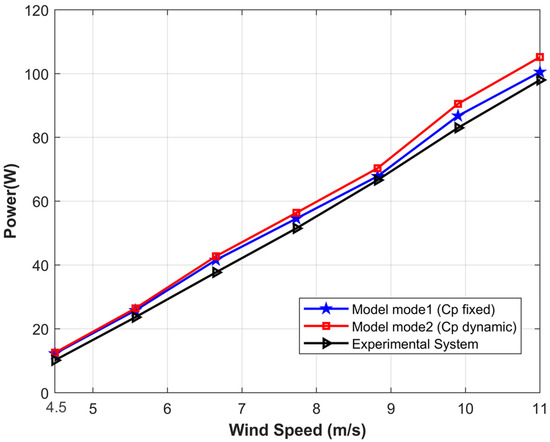
Figure 7.
Comparison between the model results and measured data from the experimental setup in this study.
The output power at the optimum Cp mode was the highest throughout the wind interval because of its dynamic ability to find the optimal and maximum value of power coefficient of each value of wind speed, resulting in lower power losses. Whereas in the fixed Cp mode, the value of the power coefficient was constant since there was no change in the tip speed ratio and the pitch angle of the wind turbine.
3.2. Model Application to a Real Case Study in Pakistan Considering the Indirect Drive Configuration
The proposed study was further enhanced to analyze the potential of wind power generation in Pakistan. The potential of wind energy is much higher than the installed capacity throughout the country. The wind energy potential in Pakistan is roughly 300 GW for electric power generation [43,44], which is around 9.3 times the country’s current installed capacity. Many wind corridors are observed across Pakistan, especially in the northern and southern parts of the country, which are shown in Figure 8. The range of wind power is classified from poor wind speed, such as 0–5.4 m/s, to excellent wind speed, such as 7.8–8.6 m/s, in different parts of the country.
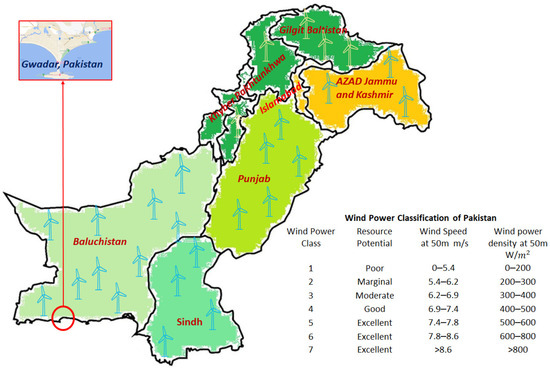
Figure 8.
Geographical map of the wind power classification at a 50 m height in different areas in Pakistan [43].
The developed model was applied to evaluate the optimal power generation from a pilot project, which hosted 20 kW wind turbines (see Table 3) in order to meet the electricity demand of a 10 kW medium-wave radio transmitter and the allied equipment of the Pakistan Broadcasting Corporation (PBC) station located in Gwadar city in the southwestern province Baluchistan, Pakistan [45], and it also helps to contribute to the 2030 renewable energy plan of Pakistan [46]. The registered average wind speed in some areas of Sindh and Baluchistan provinces in autumn was 3.9 m/s, and at the beginning of summer, it is significantly higher at about 10 m/s [43]. In addition, based on the collected data, the wind speed fluctuated from 0.58 to 20.07 m/s from September 2017 to October 2018, which is classified as an excellent wind speed at a 20 m height from surface level [47].
Table 3.
Technical specification of the 20 kW wind turbine model.
The capacity of the power generated by the wind turbine is primarily dependent on the swept area of the turbine. However, the rational speed is a function of the square of turbine radius and angular speed, which is increased by decreasing the diameter of the swept area and increased since the value of TSR increased. Thus, the mutual relation of mechanical power with the turbine blade radius is directly proportional, while the angular speed is inversely proportional to blade radius, which causes the speed deviation between the turbine shaft and electric generator.
In order to obtain the nominal power of a 20 kW generator, a gear stage was used in the indirect coupling design of the wind turbine power train. For this reason, the gear stage helped to reduce the deviation gap between aerodynamic and electric machine speed and assisted in increasing the rpm for maximum power generation of a 20 kW electric machine. In other words, the wind turbine shaft drove a generator through a gearbox stage at the required speed to rotate from 1000 to 1500 rpm for an optimal operation and good efficiency of a four-pole electric machine [50]. Figure 9 shows the distribution of power losses based on the optimal value of Cp for the selected 20 kW indirect drive wind turbine. In addition, based on numerical values of model results, the cumulative power of effective and losses in a direct and indirect transmission configuration of a wind turbine was slightly different. For example, the daily cumulative electricity produced by the direct coupling-based power train was 137.03 kWh. While, in the case of a gearbox driveline, it was nominally higher at 139.57 kWh, which indicated the value of Cp had improved by regulating the angular speed through a gearbox to produce more electricity, which was 1.8% higher than the direct-drive wind turbine. On the other hand, the involvement of the gearbox itself caused the power drop along with more power loss in the PMSG and power electronics stage due to an increase in angular speed and linear frequency.
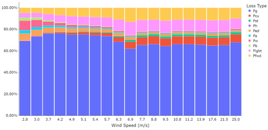
Figure 9.
Distribution of the power loss in different stages of the indirect drive wind turbine.
Figure 10 represents the model results for a 20 kW wind turbine installed in Gwadar city. Figure 10a illustrates the one-year wind profile from October 2017 to September 2018, where the wind speed varied in terms of the monthly average from 1.3 m/s to 11 m/s [46]. Figure 10b represents the behavior of the decision variables of the model. The pitch angle value varied from 0 to 1.5 degrees in the direct-drive configuration, and the tip speed ratio ranged from 7.5 to 8.3. Similarly, the value of Cp varied from 0.01 to a maximum value of 0.48. However, the change in pitch angle in the indirect coupling was slightly higher at 1.7 degrees, and the value of TSR decreased to approximately 6, which was higher in terms of the pitch angle and lower regarding the TSR compared with direct coupling. Thus, the pitch angle influenced the TSR in the gear stage coupling to obtain the maximum value of power coefficient under changing wind regimes.
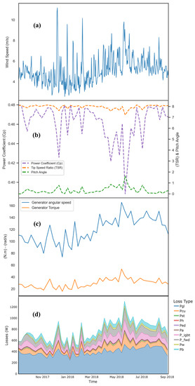
Figure 10.
Model results for a 20 kW indirect drive wind turbine installed in Gwadar city: (a) wind speed, (b) behavior of decision variables, (c) generator torque and angular speed, and (d) power losses.
In the indirect coupling configuration, the aerodynamic angular speed and torque are functions of the gear ratio, as its role is to change the speed and torque from one stage to another stage, such as from lower to higher, or vice versa. Usually, the angular speed is lower and aerodynamic torque is higher on the turbine side, depending on the blade radius. On the other hand, once the gear stage is involved in the turbine power train, both parameters changed their scales, i.e., the angular speed of the generator became higher and varied from 75 to 160 rad/s, and the torque level decreased from 50 to 10 N-m during the available wind regime, as shown in Figure 10c.
Figure 10d illustrates the power losses in different stages of a wind turbine based on the available range of wind speed, i.e., 0 to 20 m/s. The wind speed peaked in December-2017 and the last quarter of 2018. Therefore, gear and bearing losses were higher in December, and eventually, the electric and power electronics losses rose in June and July. The highest power loss occurred at approximately 1200 W at the end of May 2018 when the wind speed was higher than the rated value of 9.3 m/s. The gear loss varied from 0 to 450 W, depending on the wind speed. At the beginning of August, the gear loss rose unsteadily and reached its maximum value of approximately 450 W due to the rapid variation of wind speed that month. The copper loss was the second highest, followed by the IGBTs losses in the turbine power train, as these were functions of the current and linear frequency, respectively. At the point of the nominal speed, i.e., 9.3 m/s, most losses reached their peak values and became constant with slight variations, such as bearing, stray load, windage, and eddy current loss. This smooth drop in power resulted from optimizing the Cp value by changing the values of the TSR and pitch angle. The cumulative annual electricity generation from the wind turbine system was estimated at 45 MWh, and the total power loss was significantly high, at around 1 MWh in a year.
4. Conclusions
This research introduced an optimization model that was based on the maximization of the wind turbine power coefficient, taking into account the detailed power losses at the different stages of the power train for both direct and indirect coupling configurations. The result of the direct driveline indicated the optimal value of Cp at 0.48 for a pitch angle of 0 degrees and a TSR of 8.1 at a wind speed of approximately 11.2 m/s in the case of a small-scale 100 W wind turbine. The comparison between the result of the optimization model and the experimental system revealed that the output power in the optimal Cp mode was the highest throughout the wind interval, resulting in lower power losses. Furthermore, the research results indicated that the direct-coupled turbine models performed better for optimizing the Cp maximization of the wind turbine system. According to the results, by implementing the indirect-coupled configuration, around 45 MWh/y electricity could be extracted from a 20 KW wind turbine based on the available real wind regime of Gwadar city (2017–2018). As a result, the amount of the power loss in the indirect coupling driveline was estimated at 1 MWh/y, highlighting the rule of the optimal value of Cp in adjusting the rotational speed of the generator in an indirect coupling driveline to produce more electricity from the wind turbine systems. Moreover, the developed model can help to quickly find the power losses in existing technology and the ongoing wind system design. Similarly, it proposed that when the speed of the wind regime was lower than the nominal speed, small-scale low power wind turbines are the suitable selection for installation in such sites. However, indirect driveline-based wind turbines are a reasonable choice for producing wind energy in high-speed wind corridors areas.
Future work could concentrate on developing a model predictive controller (MPC) for the current optimization study to force the power coefficient to follow the reference trajectory, therefore, to draw the maximum aerodynamic power against the precise change in wind speed.
Author Contributions
Conceptualization and methodology: K.S. and H.F.; Investigation: K.S.; Writing: K.S. and H.F.; Review and editing: H.F.; Supervision: H.F. All authors have read and agreed to the published version of the manuscript.
Funding
This research was supported by the Japanese Grant Aid for Human Resource Development (JDS) Japan–Pakistan.
Institutional Review Board Statement
Not applicable.
Informed Consent Statement
Not applicable.
Data Availability Statement
Not applicable.
Conflicts of Interest
The authors declare no conflict of interest.
References
- Yoshida, Y.; Farzaneh, H. Optimal design of a stand-alone residential hybrid microgrid system for enhancing renewable energy deployment in Japan. Energies 2020, 13, 1737. [Google Scholar] [CrossRef]
- Esteban, M.; Portugal-Pereira, J.; Mclellan, B.C.; Bricker, J.; Farzaneh, H.; Djalilova, N.; Ishihara, K.N.; Takagi, H.; Roeber, V. 100% renewable energy system in Japan: Smoothening and ancillary services. Appl. Energy 2018, 224, 698–707. [Google Scholar] [CrossRef]
- Hinokuma, T.; Farzaneh, H.; Shaqour, A. Techno-economic analysis of a fuzzy logic control based hybrid renewable energy system to power a university campus in Japan. Energies 2021, 14, 1960. [Google Scholar] [CrossRef]
- Ugranli, F.; Karatepe, E. Optimal wind turbine sizing to minimize energy loss. Int. J. Electr. Power Energy Syst. 2013, 53, 656–663. [Google Scholar] [CrossRef]
- Hung, D.Q.; Mithulananthan, N.; Bansal, R.C. Analytical strategies for renewable distributed generation integration considering energy loss minimization. Appl. Energy 2013, 105, 75–85. [Google Scholar] [CrossRef]
- Ochoa, L.F.; Harrison, G.P. Minimizing energy losses: Optimal accommodation and smart operation of renewable distributed generation. IEEE Trans. Power Syst. 2011, 26, 198–205. [Google Scholar] [CrossRef]
- Chen, W.H.; Wang, J.S.; Chang, M.H.; Mutuku, J.K.; Hoang, A.T. Efficiency improvement of a vertical-axis wind turbine using a deflector optimized by Taguchi approach with modified additive method. Energy Convers. Manag. 2021, 245, 114609. [Google Scholar] [CrossRef]
- Baran, J.; Jaderko, A. A method of maximum power point tracking for a variable speed wind turbine system. In Proceedings of the 2019 Applications of Electromagnetics in Modern Engineering and Medicine (PTZE), Janow Podlaski, Poland, 9–12 June 2019; Volume 2, pp. 13–16. [Google Scholar] [CrossRef]
- Vijayalakshmi, S.; Ganapathy, V.; Vijayakumar, K.; Dash, S.S. Maximum Power Point Tracking for Wind Power Generation System at Variable Wind Speed using a Hybrid Technique. Int. J. Control Autom. 2015, 8, 357–372. [Google Scholar] [CrossRef][Green Version]
- Yaakoubi, A.E.; Amhaimar, L.; Attari, K.; Harrak, M.H.; Halaoui, M.E.; Asselman, A. Non-linear and intelligent maximum power point tracking strategies for small size wind turbines: Performance analysis and comparison. Energy Rep. 2019, 5, 545–554. [Google Scholar] [CrossRef]
- Pande, J.; Nasikkar, P.; Kotecha, K.; Varadarajan, V. A review of maximum power point tracking algorithms for wind energy conversion systems. J. Mar. Sci. Eng. 2021, 9, 1187. [Google Scholar] [CrossRef]
- Xia, Y.; Yin, M.; Li, R.; Liu, D.; Zou, Y. Integrated structure and maximum power point tracking control design for wind turbines based on degree of controllability. JVC J. Vib. Control 2019, 25, 397–407. [Google Scholar] [CrossRef]
- Lanzafame, R.; Messina, M. Horizontal axis wind turbine working at maximum power coefficient continuously. Renew. Energy 2010, 35, 301–306. [Google Scholar] [CrossRef]
- Wei, L.; Zhan, P.; Liu, Z.; Tao, Y.; Yue, D. Modeling and analysis of maximum power tracking of a 600 kW hydraulic energy storage wind turbine test rig. Processes 2019, 7, 706. [Google Scholar] [CrossRef]
- Adams, T.M.; Mertz, B.E. Horizontal Axis Wind Turbine Power Coefficient as Relative Capture Area. J. Fluid Flow Heat Mass Transf. 2021, 8, 254–261. [Google Scholar] [CrossRef]
- Sohoni, V.; Gupta, S.C.; Nema, R.K. A Critical Review on Wind Turbine Power Curve Modelling Techniques and Their Applications in Wind Based Energy Systems. J. Energy 2016, 2016, 8519785. [Google Scholar] [CrossRef]
- Chinamalli, P.K.S.; Naveen, T.S.; Shankar, C.B. Power Loss Minimization of Permanent Magnet Synchronous Generator Using Particle Swarm Optimization. Int. J. Mod. Eng. Res. 2021, 2, 4069–4076. Available online: http://www.ijmer.com/papers/Vol2_Issue6/AO2640694076.pdf (accessed on 1 December 2021).
- Lap-Arparat, P.; Leephakpreeda, T. Real-time maximized power generation of vertical axis wind turbines based on characteristic curves of power coefficients via fuzzy pulse width modulation load regulation. Energy 2019, 182, 975–987. [Google Scholar] [CrossRef]
- Song, D.; Liu, J.; Yang, Y.; Yang, J.; Su, M.; Wang, Y.; Gui, N.; Yang, X.; Huang, L.; Joo, Y.H. Maximum wind energy extraction of large-scale wind turbines using nonlinear model predictive control via Yin-Yang grey wolf optimization algorithm. Energy 2021, 221, 119866. [Google Scholar] [CrossRef]
- Jia, L.; Hao, J.; Hall, J.; Nejadkhaki, H.K.; Wang, G.; Yan, Y.; Sun, M. A reinforcement learning based blade twist angle distribution searching method for optimizing wind turbine energy power. Energy 2021, 215, 119148. [Google Scholar] [CrossRef]
- Santiago, J.A.E.; Danguillecourt, O.L.; Duharte, G.I.; Díaz, J.E.C.; Añorve, A.V.; Hernandez Escobedo, Q.; Enríquez, J.P.; Verea, L.; Galvez, G.H.; Portela, R.D.; et al. Dimensioning optimization of the permanent magnet synchronous generator for direct drive wind turbines. Energies 2021, 14, 7106. [Google Scholar] [CrossRef]
- Inoue, A.; Ali, M.H.; Takahashi, R.; Murata, T.; Tamura, J.; Kimura, M.; Futami, M.; Ichinose, M.; Ide, K. A calculation method of the total efficiency of wind generator. In Proceedings of the 2005 International Conference on Power Electronics and Drives Systems, Kuala Lumpur, Malaysia, 28 November–1 December 2005; Volume 2, pp. 1595–1600. [Google Scholar] [CrossRef][Green Version]
- Cui, J.; Liu, S.; Liu, J.; Liu, X. A comparative study of MPC and economic MPC of wind energy conversion systems. Energies 2018, 11, 3127. [Google Scholar] [CrossRef]
- Telecommunications, C.; Crawford, T.; Hill, G. A Low-Speed, High-Torque, Direct-Drive Permanent Magnet Generator for Wind Thrbines. In Proceedings of the Conference Record of the 2000 IEEE Industry Applications Conference. Thirty-Fifth IAS Annual Meeting and World Conference on Industrial Applications of Electrical Energy, Rome, Italy, 8–12 October 2000; pp. 147–154. [Google Scholar]
- Huynh, C.; Zheng, L.; Acharya, D. Losses in high speed permanent magnet machines used in microturbine applications. J. Eng. Gas Turbines Power 2009, 131, 2–7. [Google Scholar] [CrossRef]
- Choi, J.Y.; Ko, K.J.; Jang, S.M. Experimental works and power loss calculations of surface-mounted permanent magnet machines. J. Magn. 2011, 16, 64–70. [Google Scholar] [CrossRef][Green Version]
- Muyeen, S.M. Wind Energy Conversion Systems: Technology and Trends; Green Energy and Technology; Springer: Berlin/Heidelberg, Germany, 2012; p. 78. [Google Scholar] [CrossRef]
- Farzaneh Laboratory. Experimental Setup, Energy and Environmental Engineering Department, Kyushu University Japan. Available online: http://farzaneh-lab.kyushu-u.ac.jp/Experiment.html (accessed on 1 December 2021).
- Desmond, C.; Murphy, J.; Blonk, L.; Haans, W. Description of an 8 MW reference wind turbine. J. Phys. Conf. Ser. 2016, 753, 9. [Google Scholar] [CrossRef]
- Gao, L.; Tao, T.; Liu, Y.; Hu, H. A field study of ice accretion and its effects on the power production of utility-scale wind turbines. Renew. Energy 2021, 167, 917–928. [Google Scholar] [CrossRef]
- Jelavić, M.; Petrović, V.; Barišić, M.; Ivanović, I. Wind turbine control beyond the cut-out wind speed. In Proceedings of the Annual Conference and Exhibition of European Wind Energy Associatio, Vienna, Austria, 4–7 February 2013; Volume 1, pp. 343–349. [Google Scholar]
- Wijewardana, S.; Shaheed, M.H.; Vepa, R. Optimum Power Output Control of a Wind Turbine Rotor. Int. J. Rotating Mach. 2016, 2016, 6935164. [Google Scholar] [CrossRef]
- Abdelqawee, I.M.; Yousef, A.Y.; Hasaneen, K.M.; Nashed, M.N.F.; Hamed, H.G. Standalone wind energy conversion system control using new maximum power point tracking technique. Int. J. Emerg. Technol. Adv. Eng. Certif. J. 2019, 9, 95–100. [Google Scholar] [CrossRef]
- Sun, H.; Han, Y.; Zhang, L. Maximum Wind Power Tracking of Doubly Fed Wind Turbine System Based on Adaptive Gain Second-Order Sliding Mode. J. Control. Sci. Eng. 2018, 2018, 5342971. [Google Scholar] [CrossRef]
- Al Ameri, A.; Ounissa, A.; Nichita, C.; Djamal, A. Power loss analysis for wind power grid integration based on Weibull distribution. Energies 2017, 10, 463. [Google Scholar] [CrossRef]
- Kjaer, A.B.; Korsgaard, S.; Nielsen, S.S.; Demsa, L.; Rasmussen, P.O. Design, Fabrication, Test, and Benchmark of a Magnetically Geared Permanent Magnet Generator for Wind Power Generation. IEEE Trans. Energy Convers. 2020, 35, 24–32. [Google Scholar] [CrossRef]
- Samraj, D.B.; Perumal, M.P. Analogy of the losses in surface and interior permanent magnet synchronous wind turbine generators. Int. J. Sci. Technol. Res. 2019, 8, 2507–2515. [Google Scholar]
- G. D. Corporation. General Algebraic Modeling System Variable Attributes about Initial, Lower, and Upper Values. Available online: https://www.gams.com/latest/docs/UG_Variables.html (accessed on 1 December 2021).
- International Rectifier. Automativ Grade. AUIRG4BC30S-S AUIRG4BC30S-S/SL Reverse Transfer Capacitance; International Rectifier: El Segungo, CA, USA, 2022; pp. 1–14. [Google Scholar]
- Pluta, W.A. Przegląd Elektrotechniczny (Electrical Review), Core Loss Models in Electrical Steel Sheets with Different Orientation. 2011, 9, pp. 37–42. Available online: http://pe.org.pl/articles/2011/9b/8.pdf (accessed on 1 December 2021).
- Mitsubishi Electric Inverter, Technical Note, No.30, Capacity Selection II [Data]. Available online: https://dl.mitsubishielectric.com/dl/fa/document/manual/inv/sh060003eng/sh060003engg.pdf (accessed on 1 December 2021).
- Shaqour, A.; Farzaneh, H.; Yoshida, Y.; Hinokuma, T. Power control and simulation of a building integrated stand-alone hybrid PV-wind-battery system in Kasuga City, Japan. Energy Rep. 2020, 6, 1528–1544. [Google Scholar] [CrossRef]
- Baloch, M.H.; Abro, S.A.; Sarwar Kaloi, G.; Mirjat, N.H.; Tahir, S.; Nadeem, M.H.; Gul, M.; Memon, Z.A.; Kumar, M. A research on electricity generation from wind corridors of Pakistan (two provinces): A technical proposal for remote zones. Sustainability 2017, 9, 1611. [Google Scholar] [CrossRef]
- Baloch, M.H.; Kaloi, G.S.; Memon, Z.A. Current scenario of the wind energy in Pakistan challenges and future perspectives: A case study. Energy Rep. 2016, 2, 201–210. [Google Scholar] [CrossRef]
- Pakistan Broadcasting Corporation (PBC), Ministry of Information and Broadcasting Government of Pakistan. Available online: http://www.moib.gov.pk/Pages/168/PBC (accessed on 1 December 2021).
- Abrar, S.; Farzaneh, H. Scenario analysis of the low emission energy system in pakistan using integrated energy demand-supply modeling approach. Energies 2021, 14, 3303. [Google Scholar] [CrossRef]
- Khlaifat, N.; Altaee, A.; Zhou, J.; Huang, Y.; Braytee, A. Optimization of a small wind turbine for a rural area: A case study of Deniliquin, New South Wales, Australia. Energies 2020, 13, 2292. [Google Scholar] [CrossRef]
- Jiao, S.; Patterson, D.; Camilleri, S. Boost Converter Design for 20KW Wind Turbine Generator. Int. J. Renew. Energy Eng. 2020, 2, 118–122. [Google Scholar]
- Mohd, M.; Shadab, A.; Mallick, M. Simulation and Control of 20 Kw Grid Connected Wind System. Int. J. 2013, 3, 275–284. Available online: http://scholar.google.com/scholar?hl=en&btnG=Search&q=intitle:SIMULATION+AND+CONTROL+OF+20+KW+GRID+CONNECTED+WIND+SYSTEM#0 (accessed on 1 December 2021).
- Abdel-Salam, M.; Ahmed, A.; Abdel-Sater, M. Maximum power point tracking for variable speed grid connected small wind turbine. In Proceedings of the 2010 IEEE International Energy Conference, Manama, Bahrain, 18–22 December 2010; pp. 600–605. [Google Scholar] [CrossRef]
Publisher’s Note: MDPI stays neutral with regard to jurisdictional claims in published maps and institutional affiliations. |
© 2022 by the authors. Licensee MDPI, Basel, Switzerland. This article is an open access article distributed under the terms and conditions of the Creative Commons Attribution (CC BY) license (https://creativecommons.org/licenses/by/4.0/).