Grid-Connected Power Converters: An Overview of Control Strategies for Renewable Energy

Abstract

The move towards a greener energy mix to fight climate change propels investments in converter-interfaced resources such as wind and photovoltaics, energy storage systems and electric vehicles. The ongoing evolution of the power system is occurring at a very fast pace, challenging transmission and distribution system operators to seek solutions that are not only adequate for this moment but also for future scenarios. Ongoing research in the fields of power electronics, power systems and control aims at developing control strategies that will help the energy transition to occur, while keeping a stable, secure and reliable power system. The objective of this paper is to present a critical review of the control strategies developed for grid-connected power converters found in renewable energy systems, energy storage systems and electric vehicles. The impact of grid-connected converters on the stability of power grids is also reviewed, highlighting the promising control strategies for enhancing system stability.

1. Introduction

Economic development and population growth are providing great opportunities for the early 21st century’s technological development. The challenge of keeping economies growing and sustaining the needs of a growing number of inhabitants, whilst envisioning the near future, where the climate crisis will play an even larger role in everyday life, calls for research in topics that enable a sustainable future for generations to come. Today, much of the electricity is generated from fossil-fuel-based generation sources [1]. Moreover, the transportation sector relies mainly on Internal Combustion Engines (ICE), which also contributes to the historically high levels of CO${}_2$ emissions recently reported.

From the power generation sector’s perspective, an environmentally friendly alternative power source is renewable energy, which is a clean energy source that does not contribute to any adverse effects on the environment [2]. Another factor that led to the increase in the search for renewable energy was the decrease in the cost of implementing the energy generation system, such as solar photovoltaics (PV) or wind energy conversion systems [3]. However, such forms of energy generation have the disadvantage of depending on environmental conditions, thus creating the need for a specific generation project for each region and its particularities [4]. Such sources provide a fluctuating energy supply, which becomes a problem to supply critical demands; these problems have led to numerous scientific research studies in the area of renewable energy [5], especially regarding the joint operation with energy storage systems (ESSs) to alleviate the intermittency challenges.

In the transportation sector, the push for environmentally friendly solutions is to substitute the ICEs for electrical motors. The power source for the electric vehicles (EVs) is a battery ESS in place of fossil fuels. This is not, however, a simple transition. Without developments in the power sector in the direction of renewable energy, EVs are recharged with power from fossil-fuel-based generators, which would only displace the source of CO₂ emissions. Moreover, the power sector would have to provide the charging infrastructure for an increased number of EVs.

Renewable energy sources, ESSs and EVs can be classified as converter-interfaced resources (CIRs). They are connected to the main grid through power converters, responsible for the conversion of direct current (DC) into alternating current (AC), or vice versa. Another important role of power converters is the management of DC voltage and current levels that can be done by DC/DC converters. In PV systems, a voltage source converter (VSC) is employed as a DC/AC converter to inject the DC current generated at the PV panels into the AC electric grid. Moreover, a DC/DC buck or boost converter might be encountered in PV farms for coupling the voltage levels of the PV panel with the ones in the DC/AC converter. In wind power applications, a Back-to-Back (B2B) converter is found in Doubly Fed Induction Generators (DFIGs) and Permanent Magnet Synchronous Generators (PMSGs). The B2B converter is composed of two VSCs with a common DC link whose function is to control the machine and to manage the power flow into the grid by controlling the DC voltage. In ESS applications, the most common converters are DC/DC converters that allow the DC voltage level to be changed for charging or discharging of the ESS and a DC/AC converter when the charging station is connected into the main AC grid.

The increasing penetration levels of CIRs are translating into significant operational challenges for system operators across the globe as they exhibit a very different interaction with the electric grid than traditional synchronous generators [6,7]. Hence, with growing shares of renewable energy and ESSs in the power system, more sophisticated control strategies are needed to maintain the reliability and stability of the power supply [8]. The traditional control strategy of CIRs is based on well-established Proportional Integral (PI) controller schemes following the grid’s phase angle for current injection. Recent advances in power electronics control, however, have explored strategies based on Model Predictive Control (MPC).

MPC is a family of control strategies that use a mathematical model of the system to predict future states and obtain the optimal control input to achieve the desired performance within a control horizon [9]. The cost function to calculate the optimal input based on the converter’s performance is usually tied with reference tracking and control efforts. Within the field of power electronics, Finite Control Set (FCS) MPC was proposed since the set of possible switching signals sent to the converter is finite [10,11], which simplifies the optimization problem. Moreover, MPC can also be combined with Repetitive Control to increase the robustness in non-ideal voltage conditions [12,13,14].

In recent years, the interest in control strategies capable of increasing the contribution of CIRs in power system stability has increased. For instance, modifications to traditional control structures to enable the participation of wind turbines have been studied in [15,16]. Another rising interest of the industry is the Grid-Forming (GFM) converters. A GFM converter is an operation mode of power converters that enable renewable energy and energy storage resources to be controlled as a voltage source rather than as a Grid-Following (GFL) current source [17]. Then, a GFM converter is able to generate its own phase angle, frequency and amplitude [18]. As a consequence, GFM converters are able to improve the frequency stability of power systems [19,20,21]. GFM converter technology is still at its early development stages and an increase in the number of works investigating it is expected in the coming years.

Considering that the development of control strategies for CIRs is an important task to be carried out to comply with the operational challenges of the near-future power system, the objective of this work is to present a review of the modeling and control of power converters in renewable energy applications. Within this context, we have included ESS and EVs, since, in order to fulfill their purpose of reducing carbon emissions, they need to be developed alongside renewable energy sources. In each section, we review the traditional PI-based control strategy and one MPC alternative. This paper is structured as follows: Section 2 presents the modeling and control of single- and two-stage PV farms. The single-stage PV farm is presented to illustrate the classic PI controller of a grid-connected VSC; the two-stage PV farm is studied with a focus on the DC/DC converter that regulates the voltage level for performing the MPPT algorithm. In Section 3, the wind turbine’s DFIG is studied to illustrate the classic and predictive control of B2B converters. While the VSC tied to the grid controls the DC voltage, the one connected to the rotor side is responsible for the MPPT algorithm. In Section 4, we focus on the control of grid-tied ESSs. The storage considered can represent a grid-tied ESS or an EV. The models and MPC controllers presented complement the ones shown for the VSC of single-stage PV farms, since they present a similar model. Finally, Section 5 discusses the influence on the power system stability of the control mode chosen for the power converter. In this section, the control scheme for the GFM is presented and the motivations to research GFM control strategies are stated. Finally, Section 6 presents the conclusions.

2. Control of Solar Photovoltaic Farms

In this section, the control of solar PV farms is discussed. At first, a discussion on the general characteristics of PV farms, such as the development status of PV installed capacity and the main topologies for interconnecting PV farms to the grid, is presented; then, a review of the control strategy for DC/AC converters for PV farms is presented; finally, we review control strategies for the DC/DC converters applied in two-stage PV farms.

2.1. Characteristics and Connection Topologies of PV Farms

The global installed capacity of PV farms has soared in the last two decades. From nearly 1 GW in 2001, solar PV capacity has increased exponentially to 707.5 GW in 2020 [22]. This sudden growth was made possible through incentive programs, declining costs of the mass production of PV panels and the investments in carbon-free power sources [23,24,25,26,27]. Integrating growing levels of PV farms to the electric grid, however, is not a straightforward task given the intermittent nature of the solar irradiance [28].

The solar irradiance is the primary resource of PV farms and its availability is subjected to cloud covering, the time of year and the time of the day [29]. Moreover, due to the PV panel’s construction, its current output, which translates into the generated power, is affected by the resource availability and the voltage applied to its terminals, as seen in Figure 1.

In the early years of the deployment of PV energy, the main objective was to extract the maximum power available to maximize the financial returns. Hence, the main strategies for controlling a PV farm are derived from MPPT schemes [30,31,32]. The MPPT for PV farms aims at producing a DC voltage reference value to be applied to the PV module that would result in maximum power extraction for the current solar irradiance condition, as given by the pink curve in Figure 1.

With the negligible share of PV power connected to the grid in the beginning of the development, the operation of PV farms concerning exclusively the injection of active power was possible. However, nowadays, the share of PV farms in some power systems cannot be neglected and changes are required for the control of PV farms [33]. Therefore, grid codes have been updated and a greater contribution to power system stability is required from PV farms. As an example, the PV-STATCOM [34] proposed the use of the inverter to supply reactive power support to the power grid at nighttime when the converter was idle. Following work extended its application to daytime [35], where the remaining capacity of the PV farm could take part in the reactive power support of the grid if necessary. Despite the increase in power losses of this type of PV farm operation [36,37,38], this modern control philosophy allows PV farms to contribute actively to system stability, as seen in [39,40,41].

There are two possible topology connections for a PV farm with implications for its operational flexibility: single-stage and two-stage connections. In a single-stage PV farm, as shown in Figure 2, a DC/AC converter is employed to convert the DC power generated by the PV module into AC power to be injected into the grid [42,43,44]. In a two-stage PV farm, as shown in Figure 3, the PV module interface with the electric grid is composed of a DC/DC converter and a DC/AC converter [43,45]. Due to the extra power converter in a two-stage PV farm, single-stage PV farms are usually more efficient. However, in two-stage PV farms, the PV panels’ output voltage associated with the MPPT algorithm is fully decoupled from the AC grid’s peak voltage, which can increase operational flexibility [37].

In Figure 2 and Figure 3, $v_{pv}$ is the voltage applied to the PV module given by the MPPT algorithm; $v_{dc}$ is the DC voltage at the DC/AC converter’s DC side in the two-stage connection; C and $C_{pv}$ are the capacitances connected to the DC/AC converter and to the PV module; $i_{abc}$ is the AC current injected into the grid; $R_f$ and $L_f$ are, respectively, the resistance and the inductance of the smoothing reactor.

The capacitor banks allocated in the DC circuit are responsible for filtering the DC current ripples and act as energy storage for the DC circuit. The value of the DC circuit capacitor banks is an important design parameter since it affects the dynamics of the DC voltage [46]. The capacitor values can be chosen following the guideline (1) proposed by [47].

$$C=\frac{S_{converter}}{4\pi f{v}_{dc,min}\mathsf{\Delta }{v}_{dc}}$$

(1)

where $v_{dc,min}$ is the minimum converter DC voltage, $S_{converter}$ is the converter apparent power, f is the AC side frequency and $\mathsf{\Delta }{v}_{dc}$ is the maximum desired ripple in the DC circuit (typically considered as 2%). For the smoothing reactor $L_f$, a typical value of 0.1 p.u. can be considered, whilst for $R_f$, a typical parasitic resistance value of 0.01 p.u. can be considered.

Next, the control strategies of the converters associated with PV farms are discussed, starting with the control of DC/AC converters.

2.2. Control of DC/AC Converters for PV Applications

To develop a controller for the DC/AC converters shown in Figure 2 and Figure 3, the starting point is a mathematical model for the main variables of the system. In this section, we present a model of the converter’s interconnection to the electric grid and of the dynamics of its DC bus voltage. Further, we discuss control structures for PV farms.

A mathematical model for the DC/AC converter’s currents can be obtained by applying the Kirchhoff voltage law to the AC side circuit:

$$L_f\frac{d}{dt}{i}_{abc}=-R_f{i}_{abc}{v}_{c,abc}-v_{g,abc}$$

(2)

where $L_f$ and $R_f$ are the filter inductance and parasitic resistance, $v_{c,abc}$ is the voltage synthesized at the converter’s terminals, $v_{g,abc}$ is the grid voltage at the point of connection and $i_{abc}$ is the converter current.

By using the model given by (2) as a starting point for a controller, the designer is faced with a challenge. In the $abc$ frame, the current references are time-varying as the converter is connected to an AC grid with sinusoidal currents. Therefore, one solution is to apply the Park Transform given by:

$$\left[\begin{array}{c}{x}_d\\ x_q\\ x_0\end{array}\right]=\frac{2}{3}\left[\begin{array}{ccc}cos\left(\theta \right)& cos(\theta -\frac{2\pi }{3})& cos(\theta +\frac{2\pi }{3})\\ sin\left(\theta \right)& sin(\theta -\frac{2\pi }{3})& sin(\theta +\frac{2\pi }{3})\\ \frac{1}{2}& \frac{1}{2}& \frac{1}{2}\end{array}\right]\left[\begin{array}{c}{x}_a\\ x_b\\ x_c\end{array}\right]$$

(3)

Hence, the following model is obtained in the $dq$ frame (assuming a balanced AC system):

$$\frac{d}{dt}{i}_d=-\frac{R_f}{L_f}{i}_d+\omega i_q+\frac{1}{L_f}(v_{c,d}-v_{g,d})$$

(4)

$$\frac{d}{dt}{i}_q=-\frac{R_f}{L_f}{i}_q-\omega i_d+\frac{1}{L_f}(v_{c,q}-v_{g,q})$$

(5)

where $\omega$ is the AC grid angular frequency.

Since the $dq$ frame is rotating at a speed $\omega$, when using a model developed in the $dq$ frame, the controller is faced with the task of following constant reference values. This is a result of a constant projection of the currents in the rotating $dq$ axis. Therefore, by employing a PI controller, it is possible to ensure zero steady state tracking error.

However, a cross-coupling between $i_d$ and $i_q$ poses a disturbance to the system. This disturbance can be dealt with considering the auxiliary inputs $\mathsf{\Delta }{v}_d$ and $\mathsf{\Delta }{v}_q$ that include a feedforward compensation as [48]:

$$\mathsf{\Delta }{v}_d=v_{c,d}-v_{g,d}+\omega L_f{i}_q$$

(6)

$$\mathsf{\Delta }{v}_q=v_{c,q}-v_{g,q}-\omega L_f{i}_q$$

(7)

Then, substituting (6) and (7) into (4) and (5), the following model is obtained:

$$\frac{d}{dt}{i}_d=-\frac{R_f}{L_f}{i}_d+\frac{1}{L_f}\mathsf{\Delta }{v}_d$$

(8)

$$\frac{d}{dt}{i}_q=-\frac{R_f}{L_f}{i}_q+\frac{1}{L_f}\mathsf{\Delta }{v}_q$$

(9)

The models given by (8) and (9) can be written as first-order transfer functions $G\left(s\right)$ given by:

$$G\left(s\right)=\frac{1}{R_f+L_{f}s}$$

(10)

The current dynamics can be controlled using a PI controller $G_i\left(s\right)$ as:

$$G_i\left(s\right)=\frac{k_{p}s+k_i}{s}$$

(11)

with $k_p=L_f/T_s$ and $k_i=R_f/T_s$[49], where $T_s$ is the desired response time for the current loop. Now, the task at hand is to obtain the reference $i_d^{\ast }$ and $i_q^{\ast }$ that the current loops should track.

Given the cascaded control structure briefly discussed at the beginning of this section, the $i_d^{\ast }$ reference value is obtained from the DC voltage control. Regarding the single-stage PV farm, the DC voltage reference is generated by the MPPT and it is applied to the PV panel to ensure maximum power operation. As for the two-stage PV farm, the DC voltage is a constant value that can be chosen by the PV farm operator according to its operation strategy.

The mathematical model of the DC voltage dynamics is obtained by observing the power balance in the DC side capacitance. The following model can be obtained for the DC voltage for both topologies [48,50]:

$$C\frac{d}{dt}{v}_{dc}=-\frac{3}{4}{i}_d-i_v$$

(12)

where $i_v$ represents the current injected by the PV panel in the single-stage PV farm or the current injected by the DC/DC converter in the two-stage PV farm.

When considering $i_v$ as a disturbance, a transfer function model can be written for (12), relating $v_{dc}$ to the reference $i_d^{\ast }$ as:

$$G_o\left(s\right)=\frac{i_d^{\ast }\left(s\right)}{v_{dc}\left(s\right)}=-\frac{3}{4C}\frac{1}{s}$$

(13)

A PI controller $G_{dc}\left(s\right)$ with the same structure as (11) can be used as an outer loop to regulate the DC voltage by changing the value of $i_d^{\ast }$. The tuning of the outer loop PI controller can be done by following the methods proposed in [48,49].

Finally, considering that the system is balanced, the reactive power reference can be translated into a reference value $i_q^{\ast }$ as:

$$i_q^{\ast }=-\frac{2\overline{Q}}{3v_{g,d}}$$

(14)

The control block diagram of the strategy using this cascaded PI controller structure is represented in Figure 4. From the contributions of $\mathsf{\Delta }{v}_d$ and $\mathsf{\Delta }{v}_q$, a voltage reference $v_{abc}^{\ast }$ is obtained and a Pulse Width Modulation (PWM) is responsible for the generation of the gating signals sent to the converter’s switches.

The simulation of a 250 kW single-stage PV farm is shown in Figure 5. The connection of the PV farm to the electric grid follows the one presented in Figure 2, with parameters given by

Table 1. Single-stage PV farm system parameters.

Parameter	Value	Unit	Parameter	Value	Unit
Peak Power	250	kW	$L_f$	20	$\mathsf{\mu }$H
$v_{pv}$ (1000 W/m${}^2$, 25 ${}^{°}$C)	510	V	$R_f$	0.37	m$\mathsf{\Omega }$
$v_{\mathsf{\Delta }}$	250	V	C	108	mF
f	60	Hz

. The considered solar irradiance profile is shown in Figure 5a. In Figure 5b, the DC voltage tracking is shown, where the reference value $v_{pv}^{\ast }$ is given by the MPPT, following the pink-crossed line in Figure 1. The cascaded PI controller scheme is able to accurately track the value for $v_{pv}$ with the irradiance variations shown. Finally, Figure 5c shows the power injected by the PV farm into the electric grid. The average power follows the solar irradiance profile of Figure 5a, reinforcing that the DC voltage controller can quickly follow the MPPT reference.

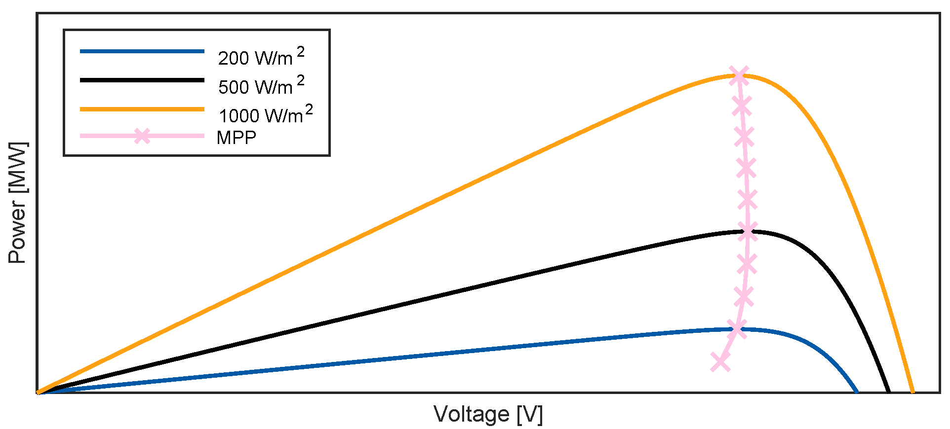
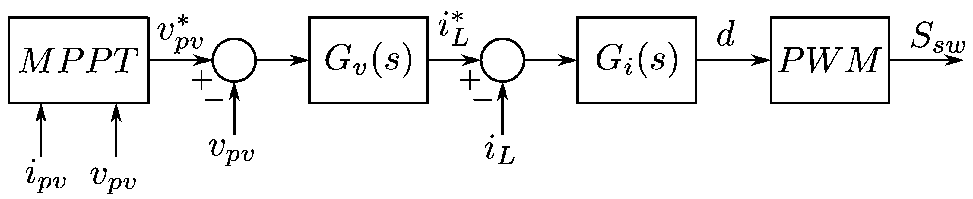
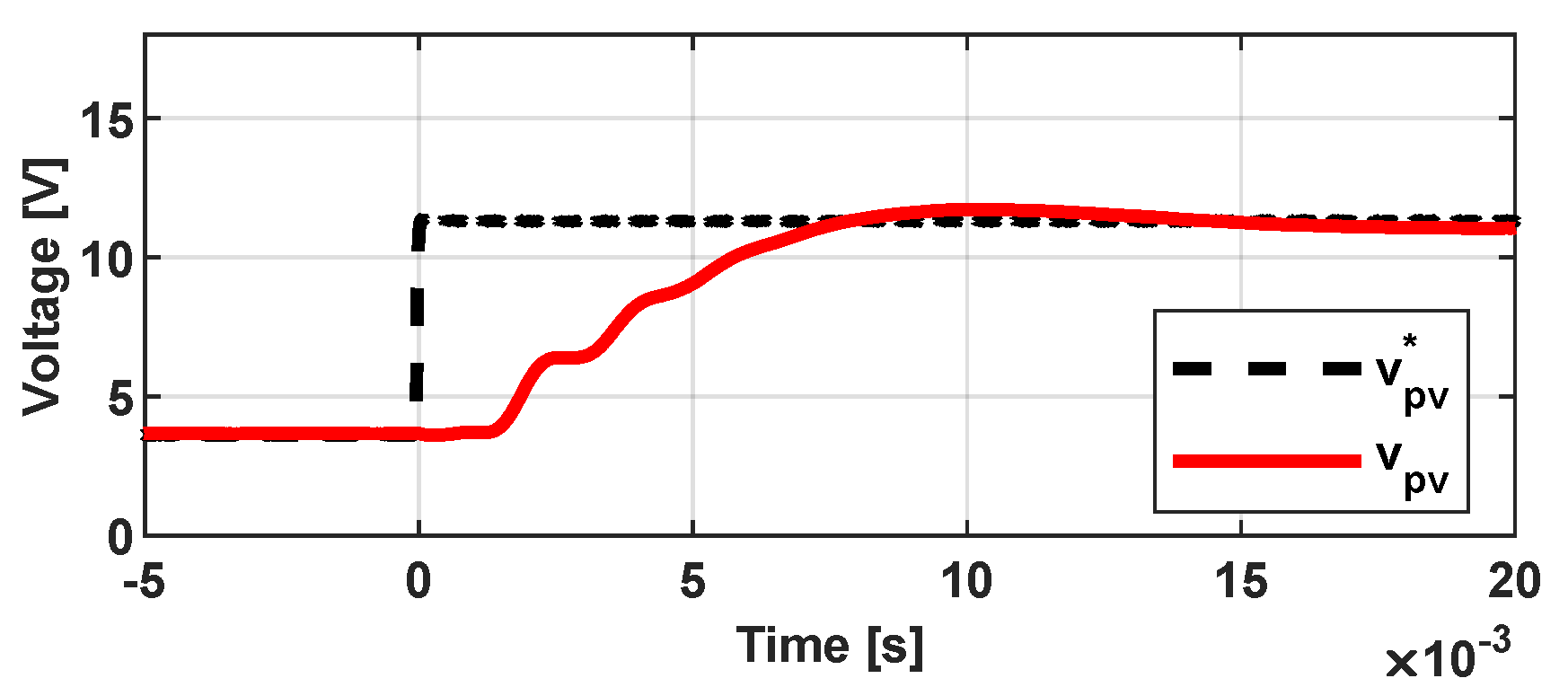
2.3. Control of DC/DC Converters for PV Applications

DC/DC converters are widely used in PV farms. Their main application is to step up the voltage of the PV array to the voltage level of a DC/AC converter in a two-stage PV farm [51,52,53] or to interface the PV panel with a DC microgrid [54,55]. In both applications, the DC/DC converter is responsible for controlling the DC voltage applied to the PV panel to operate in the reference value provided by an MPPT algorithm. In this work, we focus on the control of the DC/DC boost converter for two-stage PV farms.

A DC/DC boost converter for PV systems is shown in Figure 6. The DC/AC converter representing the second stage is assumed to be an ideal voltage source.

The modeling of boost DC/DC converters is not a straightforward task [56,57]. The system changes states as the switch turns on and off [58,59]. An average model of the system given by (15) and (16) can be obtained by using averaging theory [60].

$$\frac{d}{dt}{v}_{pv}=-\frac{1}{R{C}_{pv}}{v}_{pv}-\frac{1}{C_{pv}}{i}_L+\frac{1}{R{C}_{pv}}{v}_{irr}$$

(15)

$$\frac{d}{dt}{i}_L=\frac{1}{L}(v_{pv}-V_{dc})+\frac{1}{L}{V}_{dc}d$$

(16)

where $v_{irr}$ is the voltage of the PV panel, $v_{pv}$ is the voltage at the PV panel’s terminals, $V_{dc}$ is the voltage of the second stage of the PV farm, R is the internal resistance of the PV panel, L is the inductance of the DC/DC converter and d is the converter duty cycle.

The structure of the model in (15), (16) suggests that the control of the boost converter can be achieved in a cascaded structure, where the outer loop is responsible for generating the reference for the current $i_L$ to steer the PV panel voltage $v_{pv}$ to its reference value given by the MPPT. Then, the inner current control loop is responsible for tracking the reference of $i_L$ by manipulating the duty cycle. The duty cycle is the input to a PWM generator responsible for determining the switching signals $S_{sw}$ for the switch sw. This control strategy is represented in the block diagram of Figure 7.

The outer and inner control loops can be designed with PI controllers using the structure given in (11). A procedure for tuning the PI controllers by using the Ziegler–Nichols method is presented in [61]. More sophisticated techniques for tuning the controllers of boost converters applied to PV systems based on optimization algorithms are presented in [62,63,64].

To avoid using an average model of the converter, more advanced control strategies were proposed for the DC/DC boost converters used in PV systems. The two most popular control strategies are based on sliding mode control [58,65,66,67] and FCS [68,69,70]. In sliding mode control approaches, the boost converter modeling takes into consideration both states of the circuit in Figure 6, depending on the position of the switch, sliding between them as the switch changes its position.

On the other hand, FCS-based control strategies, as a member of the MPC family, take advantage of a model of the system and the limited number of possible states to solve an optimization problem to choose if the switch must be on or off. Moreover, the design of FCS controllers follows comprehensible steps and their design is fairly simple. As an example, the FCS control strategy proposed by [70] is shown in Figure 8.

In Figure 8, (18) and (17) are given by:

$$d\left(k\right)=\frac{1}{V_{dc}}\left[V_{dc}+L\frac{i_L(k+1)-i_L\left(k\right)}{T_{sw}}-v_{pv}\left(k\right)\right]$$

(17)

$$i_L(k+1)=i_{pv}\left(k\right)-C_{pv}\frac{v_{pv}(k+1)-v_{pv}\left(k\right)}{T_{sw}}$$

(18)

where the argument k explicitly indicates the discrete time nature of the control strategy and $T_{sw}$ is the switching frequency.

As seen in Figure 8, the MPPT provides $v_{pv}(k+1)$, the desired voltage to be applied to the terminals of the PV model, at the next time step to ensure that the maximum power is extracted. In this sense, $v_{pv}(k+1)$ can be interpreted as a reference value for the voltage $v_{pv}$. Then, (17) is used to predict the value of the inductor current in the next time step if the PV panel is operating at the $v_{pv}(k+1)$ voltage given by the MPPT. Finally, the duty cycle d can be obtained from (18), driving the DC/DC converter towards the desired value for the inductor current $i_L(k+1)$. The desired duty cycle is then used as an input to the PWM generator to obtain the switching signals $S_{sw}$ for the switch sw. At each sample, as new measurements become available, the process is repeated.

To illustrate the behavior of the FCS controller shown in Figure 8, the experimental setup used in [70] was subjected to step changes in the inductor current and in the voltage applied to the PV panel side. In Figure 9, the behavior of the inductor current of the DC/DC converter is shown when a step change is applied to the reference value $i_L^{\ast }$. The controller is able to track the reference change within 2 ms.

When the step change is applied to the reference $v_{pv}^{\ast }$, the FCS controller is able to regulate the voltage applied to the PV panel $v_{pv}$ within 10 ms, as seen in Figure 10. The voltage controller is five times slower than the current controller, explicitly showing the time-scale separation between the two cascaded loops.

3. Control of Doubly Fed Induction Generator-Based Wind Turbines

This is a dynamic model; therefore, it serves to analyze and study the transient behavior of the Doubly Fed Induction Generator (DFIG) and, more importantly, to lay the groundwork for the subsequent development of machine control. Through this dynamic model, it is also possible to know the behavior of the machine in steady state and, in general, it is possible to determine the continuous performance of the machine and the behavior of its variables, such as torque, currents and magnetic fluxes, under certain supply voltage conditions.

Likewise, the use of this information makes it possible to know how the transition from one state to another will take place, being able to detect unsafe behaviors, such as instabilities and high transient currents, in addition to providing information on dynamic oscillations, torque or current ripples, among others.

3.1. DFIG’s Mathematical Model in the Synchronous Frame (dq)

According to the AC machine models developed and discussed by different authors, such as [71], a model for the DFIG can be obtained by assuming that the three-phase system is symmetrical, the permeability of iron is infinite, the machine is magnetically linear, the resistances and reactances are constant, the voltages and currents are sinusoidal in steady state and, finally, that the effect of the harmonics in the iron is not considered. The model is obtained by writing Kirchhoff laws for the equivalent circuits in the $abc$ frame and can subsequently obtained in the $dq$ (or synchronous) reference frame by applying a Park transformation.

As detailed in [71], the DFIG’s mathematical model in the synchronous frame of reference “$dq$” is given by (19)–(23).

$${\overrightarrow{v}}_{dq,s}=R_s{\overrightarrow{i}}_{dq,s}+\frac{d{\overrightarrow{\psi }}_{dq,s}}{dt}+j{\omega }_s{\overrightarrow{\psi }}_{dq,s}$$

(19)

$${\overrightarrow{v}}_{dq,r}=R_r{\overrightarrow{i}}_{dq,r}+\frac{d{\overrightarrow{\psi }}_{dq,r}}{dt}+j\left({\omega }_s-{\omega }_m\right){\overrightarrow{\psi }}_{dq,r}$$

(20)

$${\overrightarrow{\psi }}_{dq,s}=L_s{\overrightarrow{i}}_{dq,s}+L_m{\overrightarrow{i}}_{dq,r}$$

(21)

$${\overrightarrow{\psi }}_{dq,r}=L_m{\overrightarrow{i}}_{dq,s}+L_r{\overrightarrow{i}}_{dq,r}$$

(22)

$$T_{em}=\frac{2}{3}\frac{p}{2}\frac{L_m}{L_s}({\psi }_{q,s}{i}_{d,r}-{\psi }_{d,s}{i}_{q,r})$$

(23)

where the subscripts $s,r$ indicate variables corresponding to the stator and the rotor, respectively; the resistance and inductance of windings is given by R and L; the mutual inductance between the rotor and the stator is given by $L_m$; the magnetic flux is represented by $\psi$; the electromagnetic torque is $T_m$; p is the number of pairs of poles; and ${\omega }_r,{\omega }_s$ and ${\omega }_m$ are, respectively, the rotor angular frequency, the synchronous speed and the rotor mechanical speed.

3.2. Stator Flux-Oriented System

The Stator Flux-Oriented Vector System is a control strategy that uses the DFIG’s mathematical model, shown in the previous section, that aligns the “$dq$” reference frame with the stator flux. Hence, it is possible to consider that $|{\overrightarrow{\psi }}_{dq,s}|={\psi }_{d,s}$ and consequently ${\psi }_{q,s}=0$, allowing us to rewrite the expressions (19) and (21) as (24) and (25), respectively.

$${\overrightarrow{v}}_{dq,s}=R_s{\overrightarrow{i}}_{dq,s}+\frac{d{\overrightarrow{\psi }}_{dq,s}}{dt}+j{\omega }_s{\psi }_{d,s}$$

(24)

$${\overrightarrow{\psi }}_{dq,s}={\psi }_{d,s}={\psi }_s=L_s{\overrightarrow{i}}_{dq,s}+L_m{\overrightarrow{i}}_{dq,r}$$

(25)

According to (25) and separating this equation for the two axes “d” and “q”, the stator currents can be written as (26) and (27) for each axis.

$$i_{d,s}=\frac{{\psi }_s}{L_s}-\frac{L_m}{L_s}{i}_{d,r}$$

(26)

$$i_{q,s}=-\frac{L_m}{L_s}{i}_{q,r}$$

(27)

When the machine is in steady state, the voltage drop across the stator resistance can be neglected and the stator voltage can be considered perpendicular and proportional to the stator flux, resulting in:

$$v_{q,s}=\mid {\overrightarrow{v}}_{dq,s}\mid =v_s;v_{d,s}=0;$$

(28)

Using this information, the expressions of the active power P and the reactive power Q of the stator in the stator flux-oriented synchronous reference frame are given by Equations (29) and (30) [71]:

$$P_s=-\frac{3}{2}\left(v_s\frac{L_m}{L_s}{i}_{q,r}\right)$$

(29)

$$Q_s=\frac{3}{2}{v}_s\left(\frac{{\psi }_s}{L_s}-\frac{L_m}{L_s}{i}_{d,r}\right)$$

(30)

This strategy offers a decoupling between the “$dq$” axes for the stator currents and powers, allowing the possibility of individually controlling the currents or powers. This strategy is very useful, as the DFIG’s stator is directly connected to the electrical system and the standard control strategy is to regulate the stator variables through the rotor currents ${\overrightarrow{i}}_{dq,r}$. The stator flux angle can be computed using a PLL [72,73].

3.3. State Space Model

The intention is to take advantage of the state space model to apply control over the rotor currents using the rotor voltages as the manipulated variables.

Thus, by substituting (26) and (27) into (22) and further inserting the result into (20), the expression (31) is obtained.

$${\overrightarrow{v}}_{dq,r}=(R_r+j\sigma L_r{\omega }_r){\overrightarrow{i}}_{dq,r}+\sigma L_r\frac{d{\overrightarrow{i}}_{dq,r}}{dt}+j\frac{L_m}{L_s}{\omega }_r{\psi }_s$$

(31)

where ${\omega }_r$ is the slip speed and the angular frequency of the rotor, given by ${\omega }_r={\omega }_s-{\omega }_m$ and $\sigma =1-(L_m^2/L_1{L}_2)$.

Now, from (31), it is possible to deduce the equations of the state space model, in which the current components $i_{d,r}$ and $i_{q,r}$ are the state variables (and also the output variables by considering the output matrix $C_c$ as an identity matrix), the voltages $v_{d,r}$ and $v_{q,r}$ are the input variables or control signals, and ${\psi }_s$ is considered as a disturbance.

In this way, the model represented in (32) is obtained.

$$\begin{array}{cc}\hfill \frac{d{\overrightarrow{i}}_{dq,r}}{dt}& =A_c{\overrightarrow{i}}_{dq,r}+B_c{\overrightarrow{v}}_{dq,r}+G_c{\overrightarrow{\psi }}_s\hfill \\ \hfill \overrightarrow{y}& =C_c{\overrightarrow{i}}_{dq,r}\hfill \end{array}$$

(32)

where

$$\begin{array}{cc}\hfill A_c& =\left[\begin{array}{cc}-\frac{R_r}{\sigma L_r}& {\omega }_r\\ -{\omega }_r& -\frac{R_r}{\sigma L_r}\end{array}\right]\hfill \\ \hfill B_c& =\left[\begin{array}{cc}\frac{1}{\sigma L_r}& 0\\ 0& \frac{1}{\sigma L_r}\end{array}\right]\hfill \\ \hfill G_c& =\left[\begin{array}{cc}0& \frac{{\omega }_r{L}_m}{\sigma L_r{L}_s}\\ -\frac{{\omega }_r{L}_m}{\sigma L_r{L}_s}& 0\end{array}\right]\hfill \end{array}$$

(33)

Discretizing the model (32) and considering T as the sampling period and k as a sampling instant, using a Zero-Order-Hold (ZOH) [74,75] without delay, the discrete model from (32) can be written as (34).

$$\begin{array}{cc}\hfill {\overrightarrow{i}}_{dq,r}(k+1)& =A_d{\overrightarrow{i}}_{dq,r}\left(k\right)+B_d{\overrightarrow{v}}_{dq,r}\left(k\right)+G_d{\overrightarrow{\psi }}_s\left(k\right)\hfill \\ \hfill \overrightarrow{y}(k+1)& =C_d{\overrightarrow{i}}_r(k+1)\hfill \end{array}$$

(34)

where

$$\begin{array}{cc}\hfill A_d& =e^{A_{c}T}\cong I+A_{c}T\hfill \\ \hfill B_d& ={\int }_0^{\tau }{e}^{A_{c}T}{B}_{c}d\tau \cong B_{c}T\hfill \\ \hfill G_d& ={\int }_0^{\tau }{e}^{A_{c}T}{G}_{c}d\tau \cong G_{c}T\hfill \end{array}$$

(35)

$$\begin{array}{cc}\hfill A_d& =\left[\begin{array}{cc}1-\frac{R_{r}T}{\sigma L_r}& {\omega }_{r}T\\ -{\omega }_{r}T& 1-\frac{R_{r}T}{\sigma L_r}\end{array}\right]\hfill \\ \hfill B_d& =\left[\begin{array}{cc}\frac{T}{\sigma L_r}& 0\\ 0& \frac{T}{\sigma L_r}\end{array}\right]\hfill \\ \hfill G_d& =\left[\begin{array}{cc}0& \frac{{\omega }_r{L}_{m}T}{\sigma L_r{L}_s}\\ -\frac{{\omega }_r{L}_{m}T}{\sigma L_r{L}_s}& 0\end{array}\right]\hfill \end{array}$$

(36)

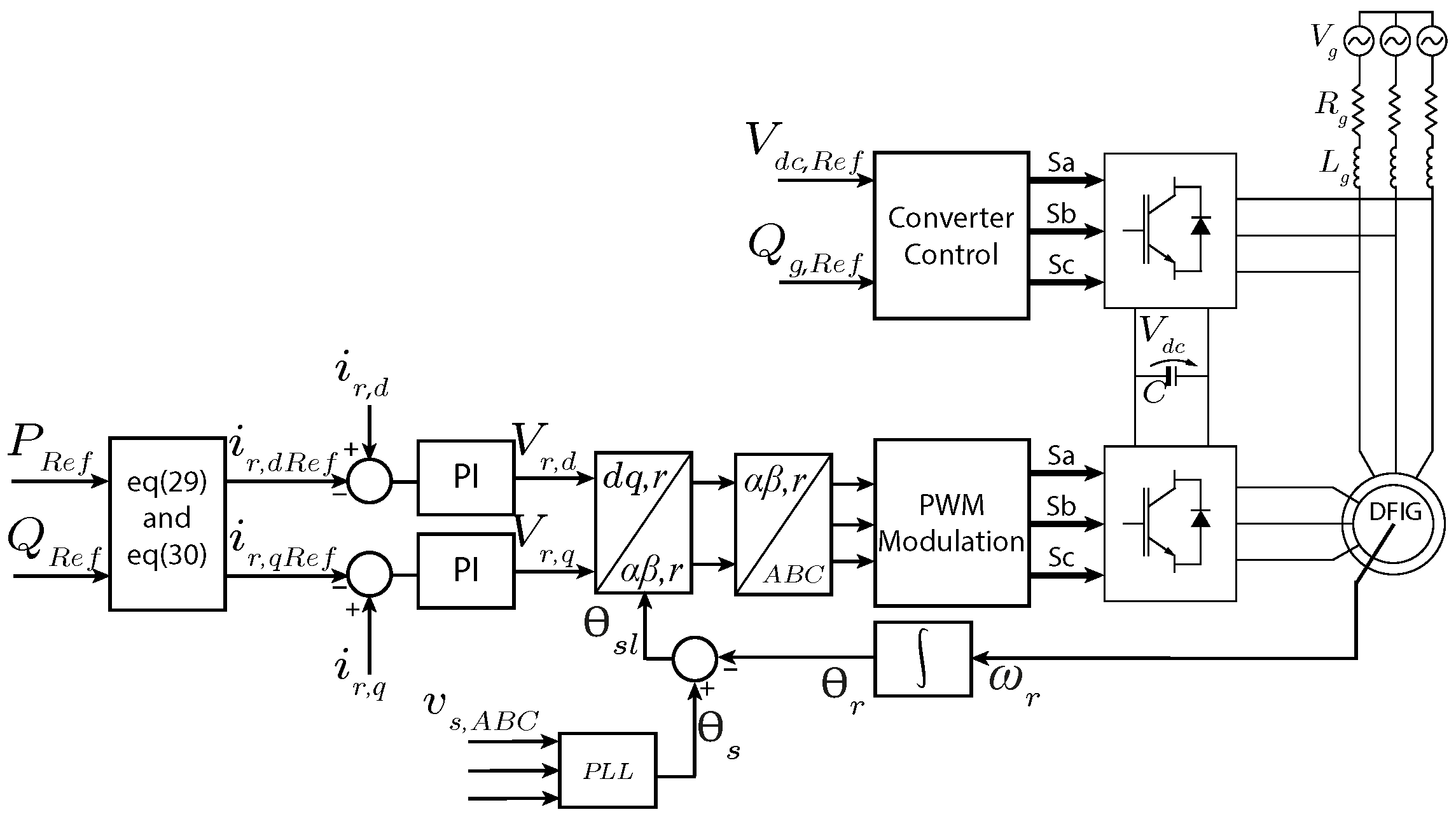
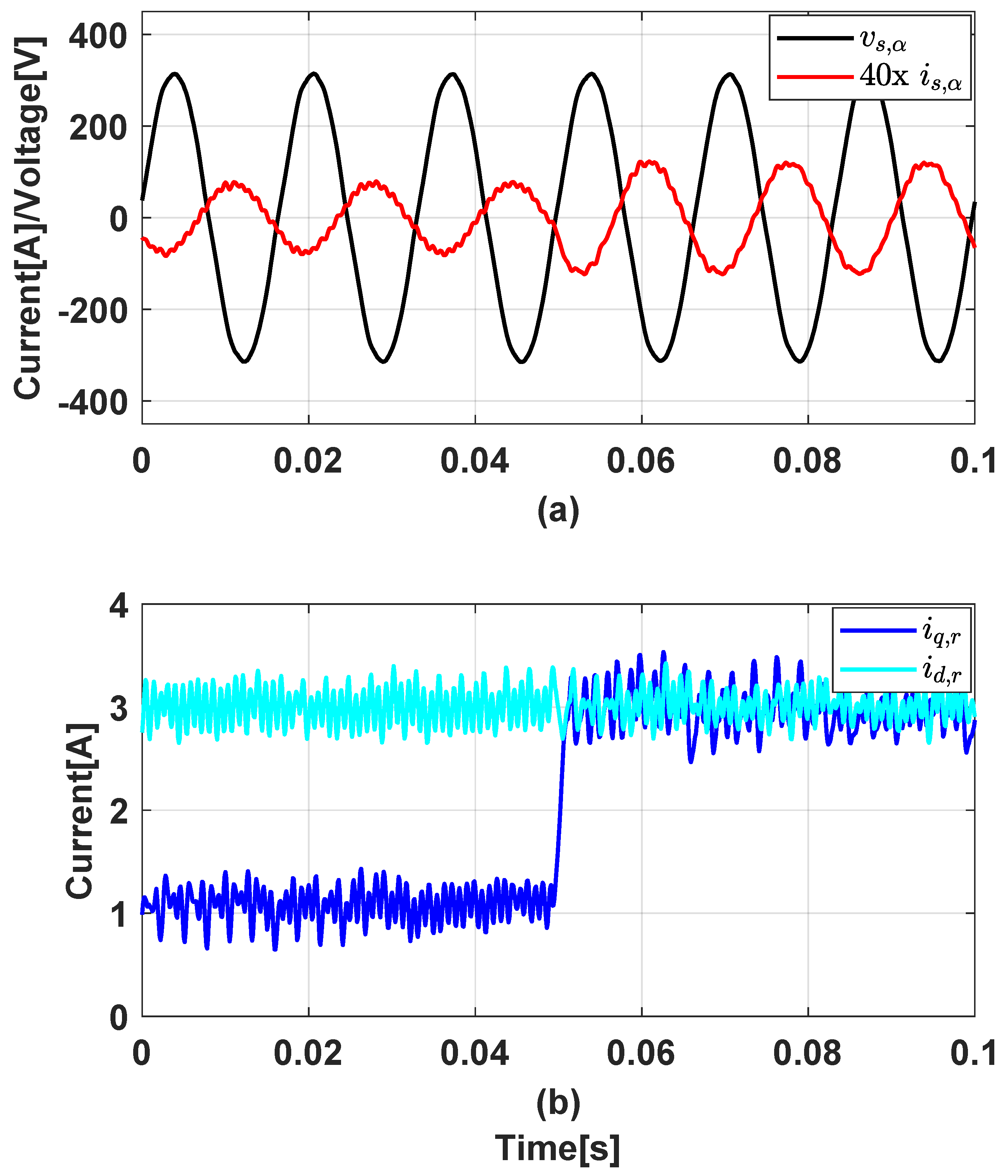
3.4. Proportional Integral Control for DFIG

For the direct power control of the DFIG, a cascaded control scheme is used to control the power produced by the DFIG, being injected or absorbed by the grid. Following the cascade scheme through Equations (29) and (30) from the active and reactive power references provides a reference value for the currents $i_d,r$ and $i_q,r$.

Finally, calculating the error between the reference currents and the measurement, a PI processes the error for both the direct axis and quadrature axis current to provide the voltage values that must be applied to the rotor through an inverter controlled by PWM.

$$V_{r,d}=({\overrightarrow{i}}_{r,dRef}-{\overrightarrow{i}}_{r,d})(k_{idP}+{\displaystyle \frac{k_{idi}}{s}})$$

(37)

$$V_{r,q}=({\overrightarrow{i}}_{r,qRef}-{\overrightarrow{i}}_{r,q})(k_{iqP}+{\displaystyle \frac{k_{iqi}}{s}})$$

(38)

The diagram presented in Figure 11 represents the full scheme for the DFIG’s direct power control using PIs.

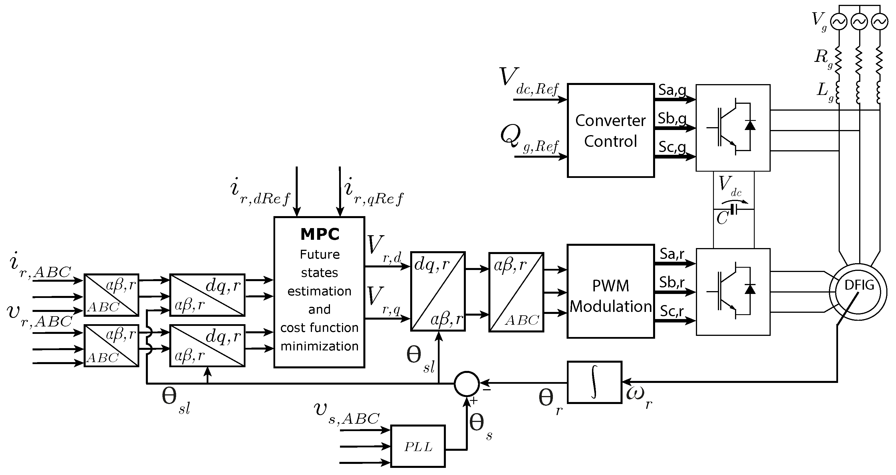
3.5. Model Predictive Control for the DFIG

An MPC controller uses a model of the system to predict its future actions and calculate the optimal inputs based on the minimization of a cost function. Additionally, it allows for the easy handling of the system’s constraints.

From the discrete state space model obtained in the previous section, the prediction of the components of the rotor current vector can be performed as [76]:

$$\begin{array}{c}\hfill {\mathrm{I}}_{\mathrm{r}}=P_{px}{\overrightarrow{i}}_{dq,r}+H\mathrm{U}+D{\overrightarrow{\psi }}_s\end{array}$$

(39)

where

$$\begin{array}{c}\hfill {\mathrm{I}}_{\mathrm{r}}={\left[\begin{array}{cccc}{i}_{dq,r}(k+1)& i_{dq,r}(k+2)& \cdots & i_{dq,r}(k+n_y)\end{array}\right]}^T\end{array}$$

(40)

$$\begin{array}{c}\hfill \mathrm{U}={\left[\begin{array}{cccc}{u}_r\left(k\right)& u_r(k+1)& \cdots & u_r(k+n_y-1)\end{array}\right]}^T\end{array}$$

(41)

$$\begin{array}{c}\hfill P_{px}={\left[\begin{array}{ccccc}{C}_d{A}_d& C_d{A}_{dig}^2& C_d{A}_{dig}^3& \cdots & C_d{A}_d^{n_y}\end{array}\right]}^T\end{array}$$

(42)

$$\begin{array}{c}\hfill H=\left[\begin{array}{cccc}{C}_d{B}_d& 0& 0& \cdots \\ C_d{A}_d{B}_d& C_d{B}_d& 0& \cdots \\ C_d{A}_d^2{B}_d& C_d{A}_d{B}_d& C_d{B}_d& \cdots \\ ⋮& ⋮& ⋮& ⋮\\ C_d{A}_d^{n_y-1}{B}_d& C_d{A}_d^{n_y-2}{B}_d& \cdots \end{array}\right]\end{array}$$

(43)

$$\begin{array}{c}\hfill D=\left[\begin{array}{cccc}{C}_d& 0& 0& \cdots \\ C_d{A}_d& C_d& 0& \cdots \\ C_d{A}_d^2& C_d{A}_d& C_d& \cdots \\ ⋮& ⋮& ⋮& ⋮\\ C_d{A}_d^{n_y-1}& C_d{A}_d^{n_y-2}& \cdots & C_d\end{array}\right]\end{array}$$

(44)

In the previous equations, $n_y$ is the prediction horizon of the grid current, and $I_g$ is the prediction of the rotor current vector.

The quadratic cost function J in matrix representation is given by:

$$\begin{array}{c}\hfill J=(I_r-I_{rRef}{)}^T{M}_y(I_r-I_{rRef})+U^T{M}_{u}U\end{array}$$

(45)

where $I_{rRef}\in R^{(n_y·q)\times 1}$ represents the rotor current vector future references, $M_y\in R^{(n_y·q)\times (n_y·q)}$ weighs the controlled grid currents (outputs) and their predictions, $M_u\in R^{n_u\times n_u}$ weighs the control efforts of inverter voltage minus rotor voltage vectors, $U\in R^{n_u\times n_u}$ is the input, and $n_u$ is the control horizon.

The expression of the minimized cost function (Equation (45)) can be represented algebraically from $\frac{\partial J}{\partial U}=0$ and isolating U. Hence, the representation is given by:

$$\begin{array}{c}\hfill U={\left(H^T{M}_{y}H+M_u\right)}^{-1}{H}^T{M}_y\left(I_{rRef}-P_{px}{I}_r\right)\end{array}$$

(46)

The rotor current vector control using MPC calculates the voltage vector of the inverter in the synchronous reference frame using Equation (46), considering the value of the rotor voltage vector components in the fundamental component frequency. This voltage vector in the rotor frame is the input of the PWM algorithm as space vector modulation. In this way, the rotor current will reach their references.

The MPC controller needs the information about the angle and the fundamental frequency component of the rotor flux to compute the appropriate voltage vector of the inverter to operate during rotor voltages.

A block diagram of the MPC control of the DFIG is shown in Figure 12.

Figure 13 presents an experimental result of the MPC control applied to DFIG.

Table 2. Parameters of the DFIG and the experimental bench.

Parameter	Value	Parameter	Value
Stator Current	12 A	Stator Voltage	220/380 $\mathsf{\Delta }$–Y
Stator Resistance	1 $\mathsf{\Omega }$	Rotor Resistance	3.1322 $\mathsf{\Omega }$
Rated Power	3 kW	Mutual Inductance	0.1917 H
Rated Speed	1800 rpm	Stator Inductance	0.2010 H
Frequency	60 Hz	Rotor Inductance	0.2010 H
Number of Poles	4	Inertia Constant	0.05 kg m${}^2$
DC Voltage	130 V	Switching Frequency	10 kHz

presents all the DFIG parameters present in the experimental bench. We show the voltage and current signal in the stationary phase, together with the current values in the synchronous reference, where it can be observed that when the current reference $i_{q,r}$ is changed from 1 to 3 A and the $i_{d,r}$ reference is kept; there is an increase in the amplitude value of the current in the stator of the machine and thus more power is injected into the grid consequently.

In addition to the MPC presented in this section in a system with normal operation, in the literature, the same type of controller has been applied in a system with disturbances. In [77,78,79,80], the authors present predictive control in a system where there is an imbalance in the voltages of the electrical grid. Another situation found in practical applications is the distortion present in the main voltage due to harmonics generated by non-linear loads, as presented in articles [14,78,81].

4. Control of Grid-Connected Energy Storage Devices and Electric Vehicles

Nowadays, electric vehicles (EV) are a sustainable transport option that generates less noise and pollution when compared to vehicles with internal combustion engines. EVs use electric motors and batteries to propel the vehicle, operating more efficiently and at lower operating costs. The advancements in lithium-ion batteries along with fast charging technology are factors that have helped in the launch of EVs [82,83].

When an EV is connected to the electric grid, it can behave as a load (when it is charging) or it can provide a greater contribution to the electric grid by behaving as a grid-connected battery at the expense of additional control loops [84]. In this latter case, the EV is considered a grid-connected ESS. When controlling the DC/AC converter of an EV, the objective of the control system is to directly regulate the apparent power elements ($S=P+jQ$) exchanged with the electrical grid. The active and reactive power references are generated by a higher control level called an energy management system (EMS). In this paper, we have considered a simple EMS in the form of a PI controller that generates the active power reference $P_{g,Ref}$ based on the the desired DC voltage $V_{RefBat}$ to be applied in the battery and a fixed reference $Q_{g,Ref}$ that can be chosen by the distribution system operator. However, more complex schemes based on MPC to obtain such references can be adopted (see [85,86]) that can help to manage the lifetime and the state of charge of the battery. The signal of the active power reference will determine if the EV behaves as load or a battery. Moreover, the possibility to inject/absorb reactive power allows for the participation in the support of the grid.

For the required additional control strategy, it is necessary to measure the voltages and currents on the grid side. To facilitate the use of classical vector control approaches, the grid currents must be in a specified referential state, $(\alpha ,\beta )$ or $(d,q)$ Hence, the phase currents $i_{g,a}$, $i_{g,b}$ and $i_{g,c}$ are transformed into vectors in the desired frame of reference. On the other hand, the grid voltage is measured and its angle detected through the Phase-Locked Loop (PLL) [87], in order to obtain the voltages in the referential state $v_{g,d}$ and $v_{g,q}$ when using the synchronous reference. This angle is used to transform the variables in the frame $(a,b,c)$ to $(d,q)$ and vice versa.

When aligning the phase a with the synchronous reference frame, the direct axis current $i_d$ directly controls the active power exchanged with the grid $P_g$; in the same way, the quadrature axis current $ig,q$ directly controls the reactive power $Q_g$ exchanged with the grid. The advantage is that the control of these two components $i_{g,d}$ and $i_{g,q}$ is independent and provides an effective means for controlling active and reactive power on the grid side [88].

Therefore, by decomposition into components, the equations of the model of the converter and filter connected to the electrical grid are obtained by:

$$v_{inv,d}=R_g{i}_{g,d}+L_g{\displaystyle \frac{d{i}_{g,d}}{dt}}-{\omega }_g{L}_g{i}_{g,q}+v_{g,d}$$

(47)

$$v_{inv,q}=R_g{i}_{g,q}+L_g{\displaystyle \frac{d{i}_{g,d}}{dt}}+{\omega }_g{L}_g{i}_{g,d}+v_{g,q}$$

(48)

where $\overrightarrow{v}$ and $\overrightarrow{i}$ are the voltage and current spatial vectors, respectively. $R_g$ and $L_g$ are the resistance and inductance of the filter, respectively; the subscripts g and $inv$ denote the electrical grid and the converter, and ${\omega }_g$ is the angular speed of the electrical grid.

From the voltage and current vectors, one can calculate the apparent power expression:

$$S_g={\displaystyle \frac{3}{2}}(P_g+j{Q}_g)={\displaystyle \frac{3}{2}}({\overrightarrow{v}}_g·{\overrightarrow{i}}_g^{\ast })$$

(49)

From (49), the active and reactive power of the grid can be calculated.

$$P_g={\displaystyle \frac{3}{2}}\Re e[{\overrightarrow{v}}_g·{\overrightarrow{i}}_g^{\ast }]={\displaystyle \frac{3}{2}}(v_{g,d}{i}_{g,d}+v_{g,q}{i}_{g,q})$$

(50)

$$Q_g={\displaystyle \frac{3}{2}}\Im m[{\overrightarrow{v}}_g·{\overrightarrow{i}}_g^{\ast }]={\displaystyle \frac{3}{2}}(v_{g,q}{i}_{g,d}-v_{g,d}{i}_{g,q})$$

(51)

Obtaining the grid model and calculating the values of active and reactive power makes possible the design of control techniques such as the Proportional Integral controller and the Predictive Control. The purpose of the control is to maintain the DC bus voltage from a reference provided by a battery management system (BMS) at a higher level of supervision to determine the charging and discharging of battery EVs.

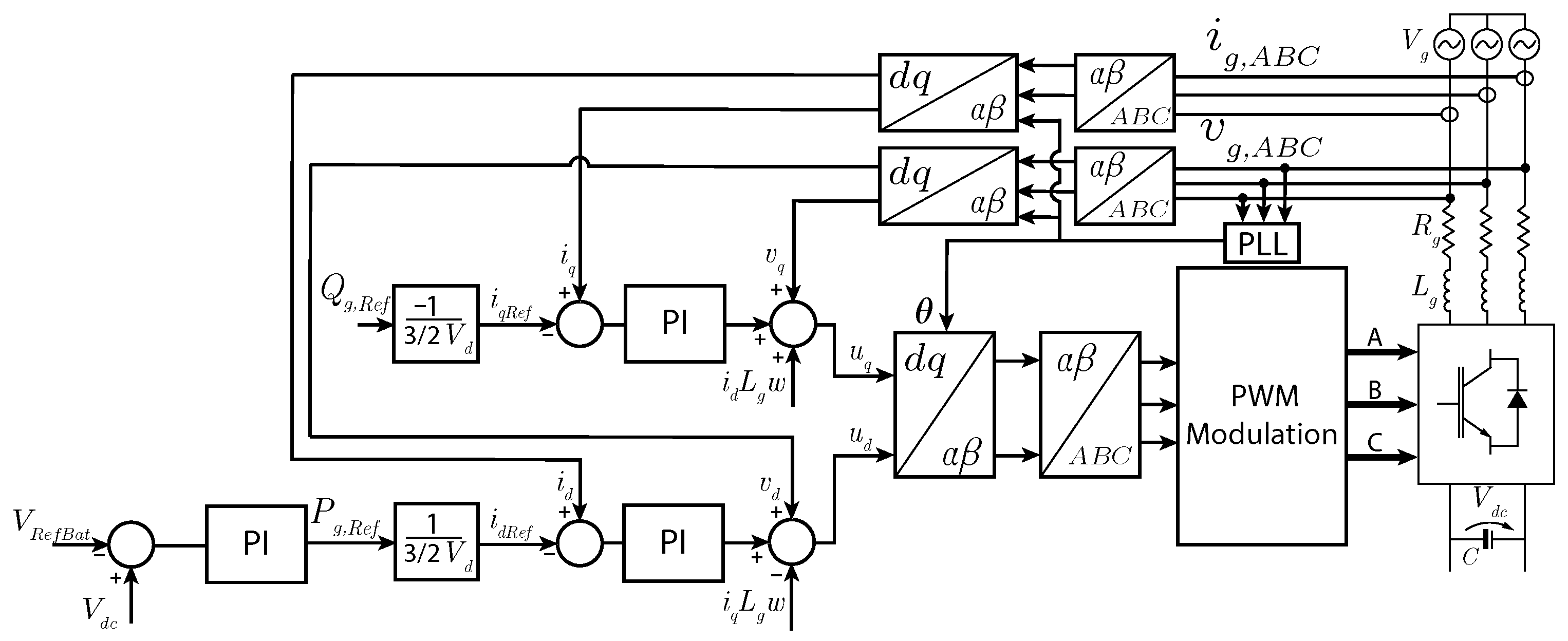
4.1. Proportional Integral Control for Storage

Figure 14 demonstrates in a block diagram the entire closed loop using proportional integral (PI) controllers [89]. From the mains voltage, the system changes to the frame $(d,q)$, thus making the active and reactive power directly proportional to the currents $i_{g,d}$ and $i_{g,q}$, since the system voltage oriented $v_d=0$ [49].

To carry out the Voltage-Oriented Control (VOC) strategy, the direct axis of the system in the synchronous reference frame $(d,q)$ is aligned with the grid voltage vector $|{\overrightarrow{v}}_{g,dq}|$, i.e., the direct axis voltage $v_{g,d}$ has the same magnitude as the grid voltage vector $|{\overrightarrow{v}}_{g,dq}|=v_{g,d}$, so the component on the quadrature axis $v_{g,q}$ is equal to zero [88].

$${\overrightarrow{v}}_{g,q}=\sqrt{|{\overrightarrow{v}}_{g,dq}{|}^2-v_{g,d}^2}=0$$

(52)

According to Equation (52), and with expressions (50) and (51), it is possible to calculate the active and reactive power that flow through the converter connected to the electrical grid and depend directly on the current vector ${\overrightarrow{i}}_{g,dq}$, as:

$$P_g={\displaystyle \frac{3}{2}}\left(v_{g,d}{i}_{g,d}\right)$$

(53)

$$Q_g=-{\displaystyle \frac{3}{2}}\left(v_{g,d}{i}_{g,q}\right)$$

(54)

From (53) and (54), it can be concluded that the active and reactive power can be controlled by controlling the direct axis and quadrature currents, respectively.

The direct axis current $i_{g,d}$ represents the active power $P_g$ on the grid side; this control loop regulates the power injected into the grid, when the converter works in steady state. The active power in the circuit is kept constant at the predetermined value $P_{g,Ref}$ as a reference; this reference is provided from a PI that calculates the error between $V_{RefBat}$ (sent from BMS) and $V_{dc}$ presented in (55).

$$P_{Refg}=(V_{RefBat}-V_{dc})(k_{vp}+{\displaystyle \frac{k_{vi}}{s}})$$

(55)

Thus, the PI controller processes the active power error $P_g$ and obtains the reference current $i_{dRef}$ through the following expression:

$$i_{dRef}=(P_{gRef}-P_g)(k_{Pp}+{\displaystyle \frac{k_{Pi}}{s}})$$

(56)

The quadrature axis current $i_{g,q}$ represents the reference reactive power $Q_{gRef}$. This reference value can be adjusted in the following ways: positive to obtain an inductive power factor, negative to obtain a capacitive power factor and zero to obtain a unity power factor. It can be calculated through the following expression:

$$i_{qRef}=(Q_{g,Ref}-Q_g)(k_{Qp}+{\displaystyle \frac{k_{Qi}}{s}})$$

(57)

With algebraic manipulation from (47) and (48), it is possible to obtain the following equation [49]:

$${\displaystyle \frac{d{i}_{g,d}}{dt}}={\displaystyle \frac{v_{inv,d}}{L_g}}-{\displaystyle \frac{v_{g,d}}{L_g}}-{\displaystyle \frac{R_g{i}_{g,d}}{L_g}}+{\omega }_g{i}_{g,q}$$

(58)

$${\displaystyle \frac{d{i}_{g,q}}{dt}}={\displaystyle \frac{v_{inv,q}}{L_g}}-{\displaystyle \frac{v_{g,q}}{L_g}}-{\displaystyle \frac{R_g{i}_{g,q}}{L_g}}-{\omega }_g{i}_{g,d}$$

(59)

where ${\omega }_g$ is the speed of the synchronous reference (grid angular frequency). Equations (58) and (59) show that the derivatives of the direct axis and quadrature axis component of the current depend on variables both on the quadrature axis and on the direct axis, respectively. This indicates that the control system is cross-coupled, which can lead to difficulties in the dynamic performance of the controller.

The coupling terms $e_{g,d}$ and $e_{g,q}$ are the voltages induced due to the three-phase transformation of the reference inductance $L_g$ to the synchronous reference $(d,q)$, and are used to improve the behavior of the system; they can be calculated as follows:

$$e_{g,d}=-{\omega }_g{L}_g{i}_{g,q}$$

(60)

$$e_{g,q}={\omega }_g{L}_g{i}_{g,d}$$

(61)

To improve the dynamic performance of the PI controllers, the voltages $U_{g,d}$ and $U_{g,q}$ of the controller decoupled from the mains can be defined as:

$$U_{g,d}=(i_{Refg,d}-i_{g,d})(k_{idP}+{\displaystyle \frac{k_{idi}}{s}})-e_{g,d}$$

(62)

$$U_{g,q}=(i_{qRef}-i_q)(k_{iqP}+{\displaystyle \frac{k_{iqi}}{s}})-e_{g,q}$$

(63)

This solution shows the independent behavior of the two control loops. Decoupled control makes the designing of PI controllers more convenient and the system is stabilized easily.

Finally, in order to be able to calculate the coordinate transformations for the voltages and currents of the electrical grid, the grid voltage angle ${\theta }_g$ is needed. With this angle, the converter can be connected to the electrical grid, and the frequency of the converter output signal must be synchronized with the frequency of the electrical grid. A technique to synchronize with the electrical grid is the phase-locked loop (PLL), which needs the three phase voltages $(a,b,c)$ of the grid, and the output of the PLL is the phase angle ${\theta }_g$ [49].

The main purpose of the PLL operation is to control the phase angle through the processing of a PI regulator; thus, the three-phase sinusoidal voltages have a transformation in the referential state $(d,q)$, through the same angle initially estimated. This quadrature axis voltage is processed by a PI controller in which the angular velocity of the electrical grid is obtained, until this signal approaches zero, thus ensuring the alignment of the direct axis d with the electrical grid vector $v_{g,dq}$, which allows us to infer that there is a synchronism between the grid and the converter.

The angular speed of the electrical grid ${\omega }_g$ can be calculated as follows:

$${\omega }_g=v_{g,q}(k_{vqP}+{\displaystyle \frac{k_{vqi}}{s}})$$

(64)

where $k_{vqP}$ and $k_{vqi}$ are the gains of the PLL controller PI. The mains angle is calculated using:

$${\theta }_g=\int {\omega }_{g}dt$$

(65)

There are PLLs that provide greater robustness to the system when it comes to harmonics distortions, as presented in [90,91,92].

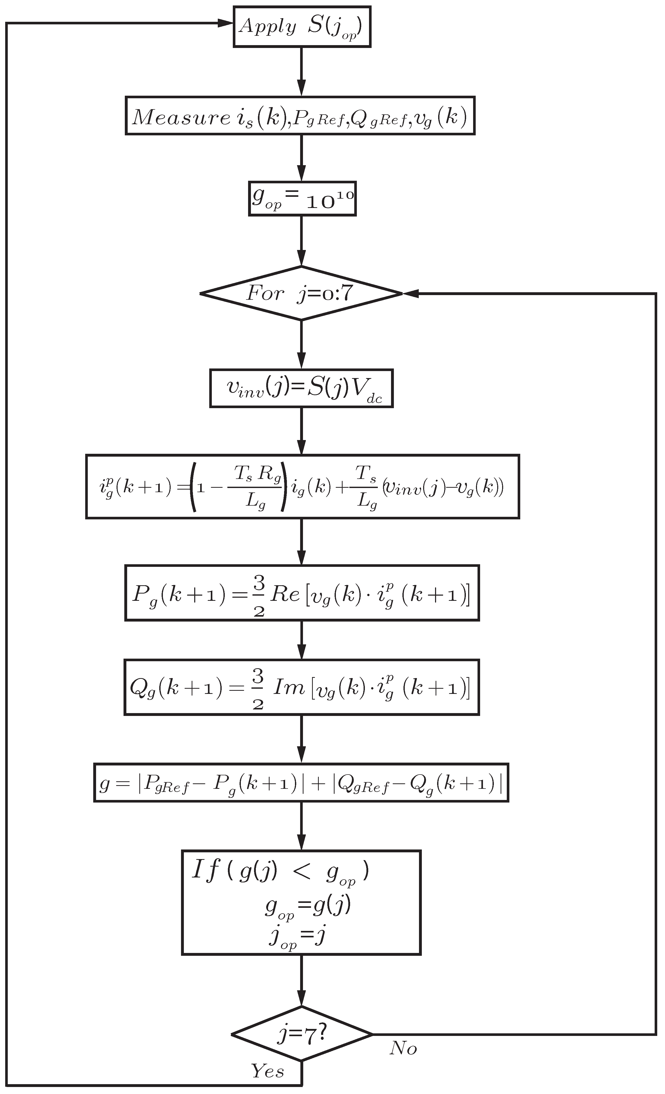
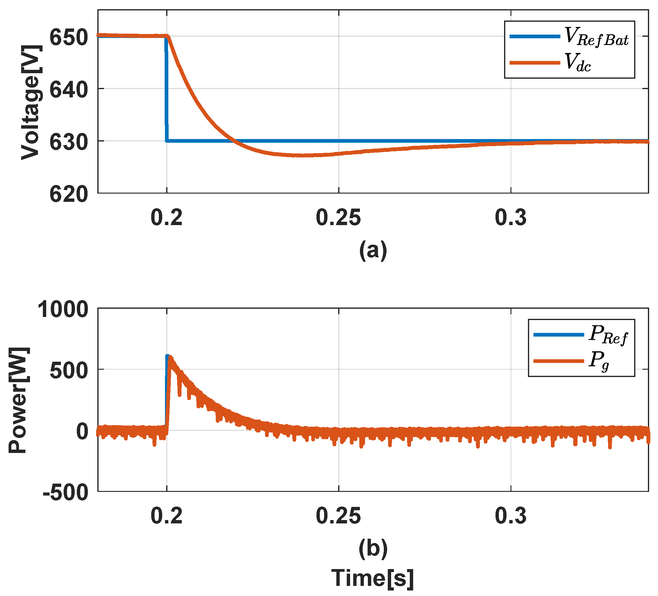
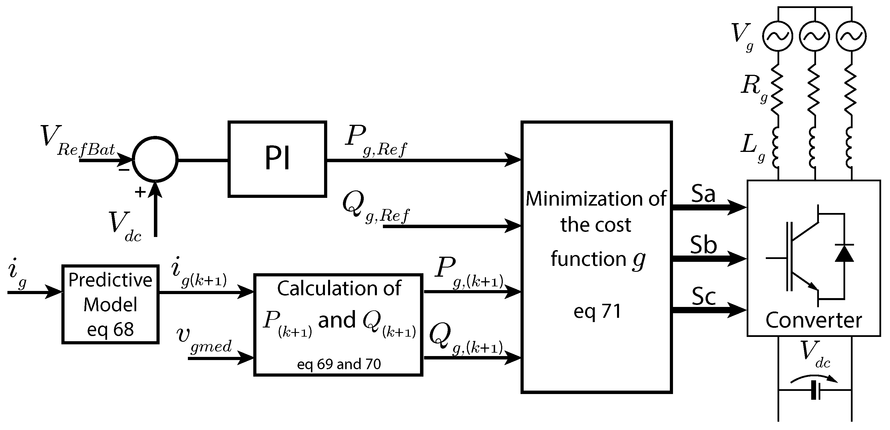
4.2. Finite Control Set Model Predictive Control (FCS-MPC) for Energy Storage Systems

FCS is a controller that falls under the umbrella of MPC. Hence, it is a control strategy that relies on a model of the system to predict its future behavior, and through minimization of a cost function, it obtains the optimal input to be applied to the system. In the case of converters based on power electronics, as is the case of the DC/AC converters found in grid-connected ESSs, FCS relies on the finite set of possible control inputs (the state of the converter switches) to evaluate every possibility to find the input that minimizes the cost function [93]. Figure 15 shows a block diagram of the inverter connected to the grid with predictive control of the type finite control set, which summarizes this control strategy for grid-connected ESSs.

An FCS-MPC controller takes advantage of the fact that the switches of the two-level DC/AC converter shown in Figure 15 can only assume a finite number of states that generate the output voltages shown in

Table 3. Switching states and voltage vectors of the inverter.

${\mathit{S}}_{\mathit{a}}$	${\mathit{S}}_{\mathit{b}}$	${\mathit{S}}_{\mathit{c}}$	Vector Voltage ${\overrightarrow{\mathit{v}}}_{{inv}}\left(\mathit{j}\right)$
0	0	0	${\overrightarrow{v}}_{inv}\left(1\right)=0$
1	0	0	${\overrightarrow{v}}_{inv}\left(2\right)=\frac{2}{3}{V}_{dc}$
1	1	0	${\overrightarrow{v}}_{inv}\left(3\right)=\frac{1}{3}{V}_{dc}+j\frac{\sqrt{3}}{3}{V}_{dc}$
0	1	0	${\overrightarrow{v}}_{inv}\left(4\right)=-\frac{1}{3}{V}_{dc}+j\frac{\sqrt{3}}{3}{V}_{dc}$
0	1	1	${\overrightarrow{v}}_{inv}\left(5\right)=-\frac{2}{3}{V}_{dc}$
0	0	1	${\overrightarrow{v}}_{inv}\left(6\right)=-\frac{1}{3}{V}_{dc}-j\frac{\sqrt{3}}{3}{V}_{dc}$
1	0	1	${\overrightarrow{v}}_{inv}\left(7\right)=\frac{1}{3}{V}_{dc}-j\frac{\sqrt{3}}{3}{V}_{dc}$
1	1	1	${\overrightarrow{v}}_{inv}\left(8\right)=0$

. The notation with the complex number j implies in this scenario that the system is modeled in the stationary reference frame.

The converter currents and voltages are obtained in the stationary frame following [11]:

$$x_{\alpha }=\frac{2}{3}\left(x_a-\frac{1}{2}{x}_b-\frac{1}{2}{x}_c\right)$$

(66)

$$x_{\beta }=\frac{2}{3}\left(\frac{\sqrt{3}}{2}{x}_b-\frac{\sqrt{3}}{2}{x}_c\right)$$

(67)

where x denotes the grid current $i_g$, the grid voltage $v_g$ or the inverter output voltage $v_{inv}$.

In discrete time, the difference equation model of the converter can be used to predict the current of the next step as [93]:

$${\overrightarrow{i}}_{g,\alpha \beta }(k+1)=\left({\displaystyle 1-\frac{T_s{R}_g}{L_g}}\right){\overrightarrow{i}}_{g,\alpha \beta }\left(k\right)+\frac{T_s}{L_g}({\overrightarrow{v}}_{inv,\alpha \beta }\left(k\right)-{\overrightarrow{v}}_{g,\alpha \beta }\left(k\right))$$

(68)

From (68), the active and reactive power exchanged by the converter with the electric grid can be predicted by:

$$P_g(k+1)=i_{g,\alpha }(k+1)·v_{g,\alpha }(k+1)+i_{g,\beta }(k+1)·v_{g,\beta }(k+1)$$

(69)

$$Q_g(k+1)=i_{g,\alpha }(k+1)·v_{g,\beta }(k+1)-i_{g,\beta }(k+1)·v_{g,\alpha }(k+1)$$

(70)

From the predicted active and reactive power values (69) and (70), the following cost function g is formulated:

$$g=|P_{g,Ref}-P_g(k+1)|+|Q_{g,Ref}-Q_g(k+1)|$$

(71)

where $P_{g,Ref}$ and $Q_{g,Ref}$ are the active and reactive power references, respectively.

Finally, since, for a short sampling time, it can be considered that $v_g(k+1)\approx v_g\left(k\right)$, the cost function (71) can be minimized by investigating the effect that the finite set of control inputs shown in Table 3 has on the cost function g by evaluating the predicted currents using (68). The vector ${\overrightarrow{v}}_{inv,\alpha \beta }$ that results in the lowest value of g is chosen and the corresponding switching is applied to the converter. Figure 16 summarizes the how the FCS-MPC algorithm works in a flowchart.

Figure 17 shows the transient response of an active power step of the implemented controller in an experimental bench using the DSP TMS320F28335, with electronic boards to condition the voltage (v) and current (i) through Hall effect magnetic sensors and a back-to-back inverter of the model “Semikron SKS20F (B6CI)2P + E1CIF + B6U 14V12” connected to the grid. To connect the inverter to the grid, there is an electrical contactor to integrate the experimental bench into the grid.

The active power step varies from 500 W to 750 W and has a settling time of around 1.8 ms. The next test presents a step in the $V_{RefBat}$ voltage and the variation of the active power provided by the PI controller of the voltage loop.

The results in Figure 17 and Figure 18 support the idea of the controller being able to follow a requested power reference when there is a variation in the bus voltage. The parameters of the experimental bench and electrical grid components are given in

Table 4. Three-phase power inverter parameters.

Parameter	Value
Inductor Internal Resistance per Phase ($R_g$)	$0.10$$\mathsf{\Omega }$
Inductance per Phase ($L_g$)	22 mH
Nominal Grid Frequency	60 Hz
Nominal Grid Voltage ($V_g$)	$78\sqrt{3}$ V
Sampling Frequency	20 kHz
Switching Frequency ($f_{sw}$)	20 kHz

. With the voltage signal coming from an external battery voltage management loop, the control proposed in the literature is able to maintain the voltage level with a fast dynamic response, since the voltage reference is reached with a time of 0.1 s. Moreover, once the bus voltage is reached, the power goes to zero until a new voltage value is sent by the battery management system.

5. Stability of Power Systems with High Penetration of Grid-Connected Converters

The dynamic characteristics of power grids have significantly altered with the increasing penetration of power-electronic converter (PEC)-interfaced generation sources, transmission and distribution systems and loads [94]. More specifically, these technologies include wind and photovoltaic generation sources, energy storage systems (e.g., battery energy storage systems, flexible ac transmission systems (FACTS), compensation devices (static-synchronous compensator (STATCOM) and static-var compensators (SVC)), high-voltage direct current (HVDC) converter stations and power electronic-interfaced loads [18,95]. Therefore, the PEC-interfaced stability issues are not only limited to generation sources, but could also originate from other PEC-interfaced devices in the power grid, such as HVDC converters and STATCOMs [94,96].

The PEC topology used in these PEC-interfaced sources plays a significant role in power grid stability. The PECs could be broadly categorized into two major types based on their topology [97,98]: (1) Grid-Forming (GFM) converters, and (2) Grid-Following (GFL) converters. The GFM and GFL converter topologies are shown in Figure 19.

Generation sources interfaced with GFM converters act as a voltage source (more precisely, as a controlled voltage source) and they can maintain the internal voltage vector constant by maintaining a constant voltage magnitude and frequency under disturbances [97]. Thus, they have a number of superior features, such as the black start capability, enhanced synchronization performance in weak grids, inertia and frequency support capability (to improve the rate-of-change-of-frequency (RoCoF) and frequency nadir [18,99,100].

However, generation sources interfaced with the GFL converters [97] are designed to follow the phase angle/frequency of the voltage waveform imposed by the synchronous generators in the power system, and inject the power into the grid according to a fixed power reference or a power reference set by the maximum power-point tracking (MPPT) system. Therefore, typically, the GFL converter-interfaced sources are not typically designed to support system inertia and reactive power requirements, and also have a small fault current contribution [101]. These features have created multifold operational and stability challenges in power grids, and the impact depends on the degree of the penetration level of GFL converters. A small penetration of GFL converters will not influence the operation of the power system, and hence their impacts can be ignored. However, when power systems begin to integrate a large number of GFL converters with high capacities, their impacts will not be restricted to the local region/area, but will begin to influence the entire power network. Subsequently, the overall dynamic performance of the power system is significantly affected. On the contrary, the GFL topology can be improved with auxiliary control schemes, such as frequency and voltage controllers, to provide enhanced support to the power grid [97]. However, their fundamental topology (i.e., GFL) remains unchanged despite these additional support services provided to the power grid.

The stability issues associated with the PEC-interfaced sources are well reported in the published literature [96]. For example, PEC-interfaced sources have influenced the transient stability [102], small-signal stability [103], voltage stability [104,105] and frequency stability [8,106]. However, the present-day stability issues originating from the PEC-interfaced sources can be broadly discussed under the following three themes:

• Low short-circuit strength and weak grid issues;
• Inertia reduction and frequency stability;
• Converter-associated interactions and resonance.

The above stability issues are discussed in detail in the following sections.

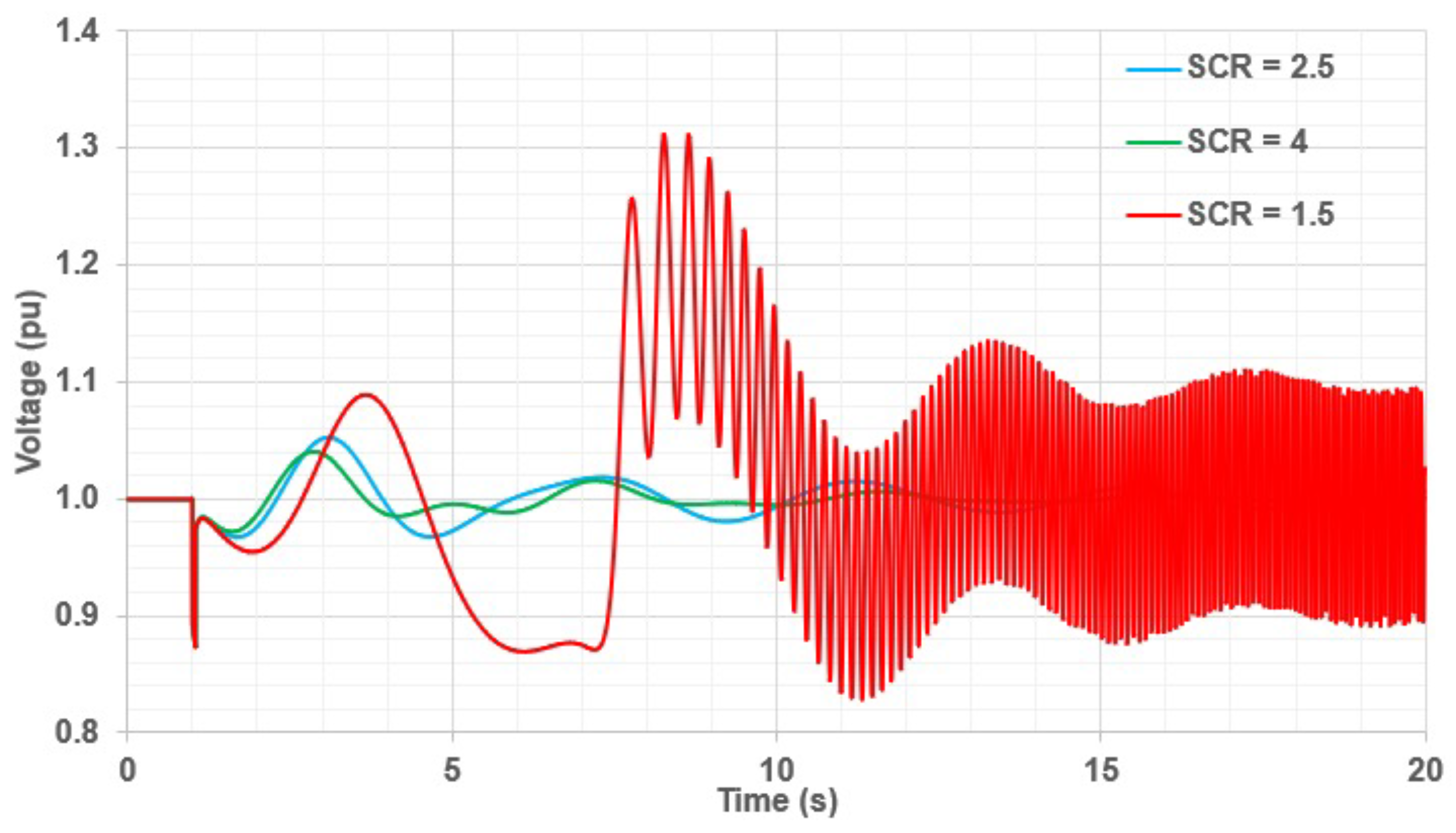
5.1. Low Short-Circuit Strength and Weak Grid Issues

Short-circuit strength is an imperative factor for power grid stability which assists in maintaining the power grid voltage following disturbances in the power grid [101]. The short-circuit strength or short-circuit capacity of a given busbar depends on the Thévenin equivalent impedance, $Z_{th}$, at that location. Hence, the short-circuit capacity (SCC) at a given location is given by:

$$Short-circuitCapacity=\frac{V_t^2}{Z_{th}}$$

(72)

where $V_t$ is the rated voltage at the busbar.

Short-circuit strength is high closer to synchronous generators and lower at remote locations (due to high Thévenin equivalent impedance). The Short-Circuit Ratio (SCR) is defined as the short-circuit capacity in MVA at the point of connection (POC) divided by the rated apparent power output in MVA of the generation source/or PEC;

$$SCR=\frac{Short-cicuitCapacity\left(inMVA\right)}{RatingoftheSource\left(inMVA\right)}$$

(73)

The effect of the short-circuit ratio was investigated considering the test system shown in Figure 20.

The test system consisted of a 1000 MVA synchronous generator connected through a 110 kV, 50 km transmission line. The rated power factor of the synchronous generator was 0.8; hence, the synchronous generator was rated at 800 MW. The synchronous generator was represented by the simple excitation system model and simple governor model. Typical parameters were considered for the synchronous generator, the excitation and the governor. The short-circuit ratio was calculated between the external grid busbar short-circuit MVA and the generator rated MVA; hence, the external grid busbar short-circuit MVA was varied to analyze the performance under different SCRs.

When the SCR falls between 3 and 2, the system is considered to be weak, and when the SCR falls below 2, the system is considered very weak. Under weak grid conditions, any small disturbance at the generation source terminal could lead to instability. Figure 21 illustrates the generation source terminal voltage under three different short-circuit ratios (SCRs).

According to Figure 21, when the SCR was at 1.5, even a 50 ms 0.12 p.u. voltage drop at the generator terminal caused the terminal voltage to oscillate and become unstable. However, in the other two instances, the terminal voltage managed to recover following the voltage drop. Other than the voltage stability issues, additional issues, such as power transfer issues and converter synchronisation issues exist, under weak grid conditions.

GFL converters contribute to weak grids from two aspects: (1) connecting at remote locations in the power grid with high Thévenin equivalent impedance; (2) low short-circuit current contribution during faults. Typically, renewable energy source and required geographical characteristics are available at remote locations; hence, GFL-based generation sources inevitably need to be situated at these remote locations. Therefore, when the penetration level of the GFL converters is significantly increased, a power system may experience weak grid issues [107]. Although the first factor is unavoidable, the second factor could be mitigated by deploying a GFM converter topology and synchronous condensers [18].

Therefore, power system operators are trying to keep the minimum required short-circuit strength to maintain power system security by keeping a minimum level of conventional synchronous generators online in the system. This is one of the limiting factors of the grid GFL converter-interfaced generator integration [108]. The rating of the GFL converter is usually determined to keep the SCR at 3 at the point of connection (POC) when the minimum number of synchronous machines are online in the system under N1 critical contingency events [109].

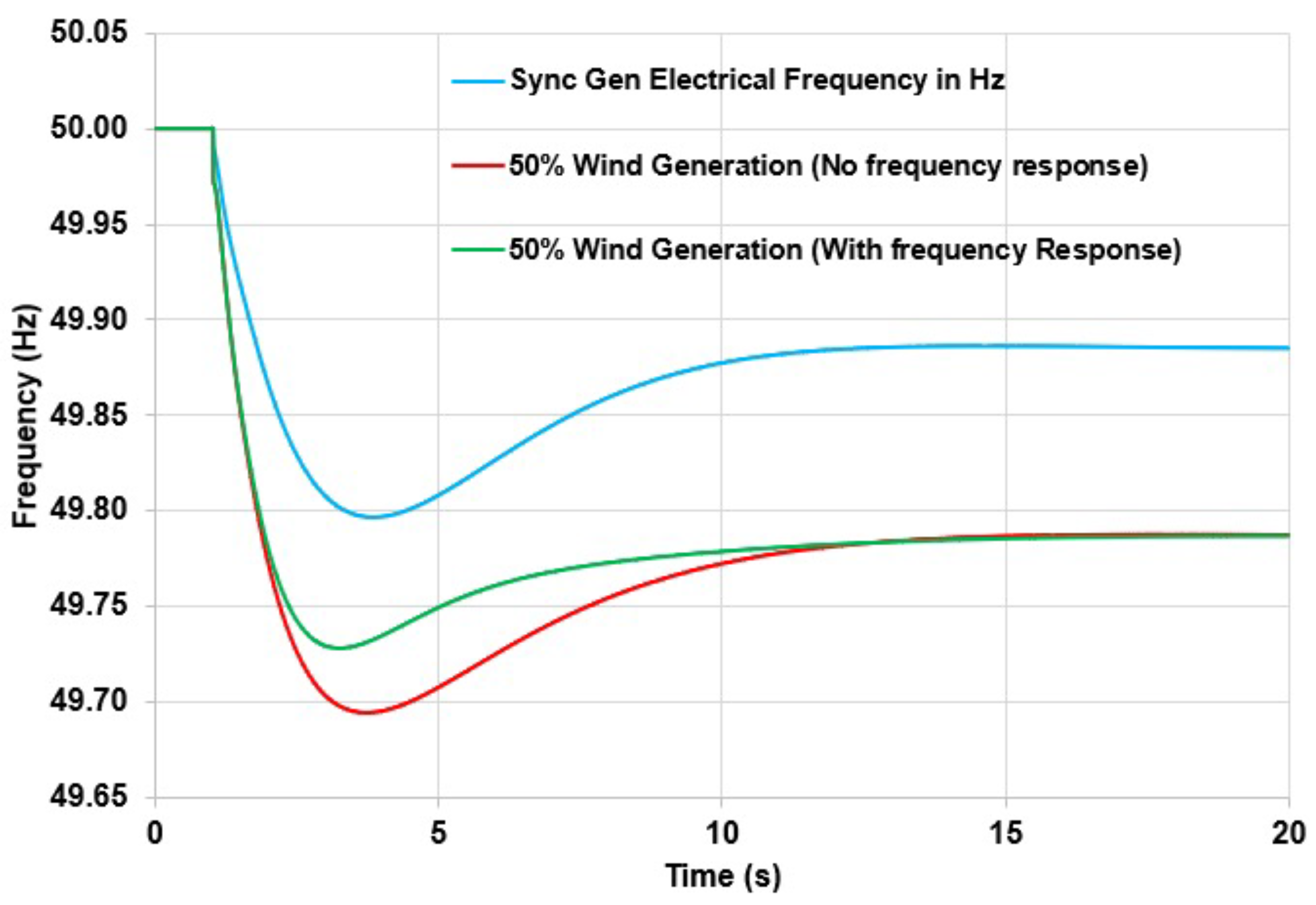
5.2. Inertia Reduction and Frequency Stability Issues

Conventional synchronous machines have an inherent inertial response capability (response proportional to RoCoF and stored energy capacity), which is a very important attribute that helps power systems to arrest the frequency drop before reaching unstable frequencies that could ultimately lead to a blackout [106]. Compared with synchronous generators, the inertia of the GFL converter is very low, due to the decoupling of the electrical dynamics of the grid and the electro-mechanical dynamics of the source by the PEC [8]. The solar PV systems do not even have stored kinetic energy as they do not have any rotating parts [110]. Thus, the future power system with a high share of PEC-interfaced generation sources no longer has the traditional inertial response characteristics based on rotational kinetic energy.

To substitute the primary frequency response capability of the synchronous generator, battery energy storage systems (BESSs) are employed in power grids [111]. However, the BESSs still have the limitation that their capacity and lifetime incrementally deteriorate when they are subjected to frequent transient power fluctuations and deep charge–discharge operation cycles [111]. Moreover, different inertial response control strategies have been developed [112,113]; however, their capability is limited due to the lack of response duration and dependency on the renewable energy source.

The system frequency response with wind generation was investigated using the test system shown in Figure 22.

The two synchronous generators (i.e., SG-1 and SG-2) were rated at 500 MVA and their active power rating was 400 MW. The two synchronous generators were represented by the steam-turbine governor model and simple excitation system model. Typical parameters were considered for the synchronous generator, the simple excitation and the steam-turbine governor. Prior to the frequency event, a 50 MW load was not connected to the network and both SG-1 and SG-2 were operating at 250 MW active power output. Then, in a 50% wind generation scenario, SG-2 was disconnected and connected a full-converter wind generator (FCWG)-based wind farm. The FCWG-based wind farm had a rated capacity of 500 MW (100 × 5 MW) and operated at 250 MW power output. The frequency response from the FCWG was obtained based on the $\mathsf{\Delta }$f-based droop approach [18].

Figure 23 illustrates the system frequency response for a low-frequency event under three (3) scenarios: (a) with synchronous generation, (b) 50% wind generation with no frequency response, (c) 50% wind generation with frequency response. The wind generation was represented by a full-converter wind generator (FCWG) and the frequency response was obtained based on the $\mathsf{\Delta }$f approach.

According to Figure 23, when 50% of the system synchronous generation was replaced by the FCWG-based wind generation, the frequency nadir dropped to 49.69 Hz, which is a 0.11 Hz drop from the synchronous generator only case. However, when the $\mathsf{\Delta }$f-based frequency response strategy was adopted, the frequency nadir was improved by 0.04 Hz, and further improvement could be achieved with a high gain for the $\mathsf{\Delta }$f-based frequency response scheme.

5.3. Other Converter-Associated Stability Issues

Among the other stability challenges, low- and high-frequency interactions and resonance issues can be considered as emerging stability challenges in the PEC-interfaced sources. Among these converter-associated stability issues, certain stability issues occur during weak grid conditions [101]. The following are the major converter-associated stability issues:

• Weak grid-driven converter-associated stability issues—The phase-locked loop and inner current control loop can destabilize the PEC under weak grid conditions, while leading to sustained oscillations in the power grid [114,115]. The PEC-interfaced generation sources and voltage source converter (VSC)-based HVDC converter systems have reported PLL-based stability issues under weak grid scenarios. High PLL gain is identified as the root cause of this instability issue [114]. Various alternative PLL schemes have been proposed to overcome these weak grid-related stability issues [116]. Moreover, inner current loop gains are also reported to be the cause of instability in PEC-interfaced sources under weak grid conditions [117].
• Fast interactions—When the PEC-interfaced sources are involved with oscillation frequencies higher than the nominal power frequency, these interactions are categorized as fast interactions. These oscillation frequencies could be high as the kHz range. There are several mechanisms by which these fast interactions could occur: (1) between PEC controllers and the passive power network elements, (2) between one PEC controller and another PEC controller or a PEC cluster, (3) between PEC controllers and other network devices, such as synchronous generators. These fast interactions are not limited to the PEC-interfaced generation sources, but also present in other PEC-interfaced devices, such as STATCOMs and HVDC systems [118,119].
• Slow interactions—The slow interactions can also originate from the same mechanisms outlined in the fast interactions category. However, the frequency range is less than the power frequency (typically less than 10 Hz); therefore, the frequency range of these interactions depends on the controller parameters and network elements. Other than these mechanisms, weak grid-related oscillations also occur at this low-frequency range, but should be analyzed under the weak grid category.
• Resonance issues—The resonance issues could arise when the network elements (series capacitors) together with the source-end impedances form a resonance circuit at sub-synchronous frequencies, leading to effective negative resistance [120]. Ultimately, this would lead to high current and voltage oscillations while damaging power grid equipment. This type of resonance condition has been reported in a number of power networks (e.g., China and ERCOT-Texas) [120], and researchers have mainly referred to these resonance issues as sub-synchronous control interactions (SSCI). Compared with the conventional resonance issues, in this particular resonance issue, PEC converters play a major role by affecting the negative resistance by PEC controllers. Therefore, the resonance condition is governed by the PEC controller.

6. Conclusions

This article provided a review of challenges and control methods in renewable energy systems. Much of the challenge lies in the intermittent nature of the energy generation, which can be partially solved with control techniques or by integrating more than one generation method into the power system. In addition to the above, some devices, such as batteries or diesel engines, can be added to the system to improve the robustness under fluctuating energy production. The control techniques presented in this work provide the necessary methodologies for the implementation of the proposed techniques and the results support the validity of the technique. The stability issues are posing threats to power grids with high renewable power generation, and they are not limited to power generation sources, but can also be applicable to other devices with a power electronic converter interface at the grid connection end. In connected systems, autonomous power generation presents a major problem in terms of power quality due to voltage and frequency fluctuations and harmonics generated by the weak grid. The article presented classic controls in generation systems focused on renewable energy based on different studies in the literature for wind, photovoltaic and grid-connected systems, in addition to the stability issues. Furthermore, instability mitigation strategies were also presented in this paper.

References

1. Zhao, Z.Y.; Chen, Y.L. Critical factors affecting the development of renewable energy power generation: Evidence from China. J. Clean. Prod. 2018, 184, 466–480. [Google Scholar] [CrossRef]
2. Fell, H.; Gilbert, A.; Jenkins, J.D.; Mildenberger, M. Nuclear power and renewable energy are both associated with national decarbonization. Nat. Energy 2022, 7, 25–29. [Google Scholar] [CrossRef]
3. Murdock, H.E.; Gibb, D.; Andre, T.; Sawin, J.L.; Brown, A.; Ranalder, L.; Collier, U.; Dent, C.; Epp, B.; Hareesh Kumar, C.; et al. Renewables 2021-Global Status Report. 2021. Available online: https://www.unep.org/resources/report/renewables-2021-global-status-report (accessed on 1 May 2022).
4. Upadhyay, S.; Sharma, M. A review on configurations, control and sizing methodologies of hybrid energy systems. Renew. Sustain. Energy Rev. 2014, 38, 47–63. [Google Scholar] [CrossRef]
5. Manzano-Agugliaro, F.; Alcayde, A.; Montoya, F.G.; Zapata-Sierra, A.; Gil, C. Scientific production of renewable energies worldwide: An overview. Renew. Sustain. Energy Rev. 2013, 18, 134–143. [Google Scholar] [CrossRef]
6. Collados-Rodriguez, C.; Cheah-Mane, M.; Prieto-Araujo, E.; Gomis-Bellmunt, O. Stability and operation limits of power systems with high penetration of power electronics. Int. J. Electr. Power Energy Syst. 2022, 138, 107728. [Google Scholar] [CrossRef]
7. Gomis-Bellmunt, O.; Sánchez-Sánchez, E.; Arévalo-Soler, J.; Prieto-Araujo, E. Principles of operation of grids of DC and AC subgrids interconnected by power converters. IEEE Trans. Power Deliv. 2020, 36, 1107–1117. [Google Scholar] [CrossRef]
8. Milano, F.; Dörfler, F.; Hug, G.; Hill, D.J.; Verbič, G. Foundations and challenges of low-inertia systems. In Proceedings of the 2018 Power Systems Computation Conference (PSCC), Dublin, Ireland, 11–15 June 2018; pp. 1–25. [Google Scholar]
9. Camacho, E.F.; Bordons, C. Introduction to model predictive control. In Model Predictive Control; Springer: Berlin/Heidelberg, Germany, 2007; pp. 1–11. [Google Scholar]
10. Rodriguez, J.; Kazmierkowski, M.P.; Espinoza, J.R.; Zanchetta, P.; Abu-Rub, H.; Young, H.A.; Rojas, C.A. State of the art of finite control set model predictive control in power electronics. IEEE Trans. Ind. Inform. 2012, 9, 1003–1016. [Google Scholar] [CrossRef]
11. Gomez, L.A.; Lourenço, L.F.; Grilo, A.P.; Salles, M.B.; Meegahapola, L.; Sguarezi Filho, A.J. Primary frequency response of microgrid using doubly fed induction generator with finite control set model predictive control plus droop control and storage system. IEEE Access 2020, 8, 189298–189312. [Google Scholar] [CrossRef]
12. Lunardi, A.; Sguarezi Filho, A.J. Current Control for DFIG Systems Under Distorted Voltage Using Predictive—Repetitive Control. IEEE J. Emerg. Sel. Top. Power Electron. 2020, 9, 4354–4363. [Google Scholar]
13. Conde D, E.R.; Lunardi, A.; Normandia Lourenço, L.F.; Sguarezi Filho, A.J. A Predictive Repetitive Current Control in Stationary Reference Frame for DFIG Systems under Distorted Voltage Operation. IEEE J. Emerg. Sel. Top. Power Electron. 2022. [Google Scholar] [CrossRef]
14. Liu, Y.; Cheng, S.; Ning, B.; Li, Y. Robust model predictive control with simplified repetitive control for electrical machine drives. IEEE Trans. Power Electron. 2018, 34, 4524–4535. [Google Scholar] [CrossRef]
15. Prieto Cerón, C.E.; Normandia Lourenço, L.F.; Solís-Chaves, J.S.; Sguarezi Filho, A.J. A Generalized Predictive Controller for a Wind Turbine Providing Frequency Support for a Microgrid. Energies 2022, 15, 2562. [Google Scholar] [CrossRef]
16. Gomez, L.; Lourenço, L.; Salles, M.; Grilo, A. Frequency support by grid connected DFIG-based wind farms. In Design, Analysis, and Applications of Renewable Energy Systems; Elsevier: Amsterdam, The Netherlands, 2021; pp. 481–496. [Google Scholar]
17. Lasseter, R.H.; Chen, Z.; Pattabiraman, D. Grid-forming inverters: A critical asset for the power grid. IEEE J. Emerg. Sel. Top. Power Electron. 2019, 8, 925–935. [Google Scholar] [CrossRef]
18. Meegahapola, L.; Mancarella, P.; Flynn, D.; Moreno, R. Power system stability in the transition to a low carbon grid: A techno-economic perspective on challenges and opportunities. Wiley Interdiscip. Rev. Energy Environ. 2021, 10, e399. [Google Scholar] [CrossRef]
19. He, X.; Pan, S.; Geng, H. Transient Stability of Hybrid Power Systems Dominated by Different Types of Grid-Forming Devices. IEEE Trans. Energy Convers. 2021, 37, 868–879. [Google Scholar] [CrossRef]
20. Lourenço, L.F.; Perez, F.; Iovine, A.; Damm, G.; Monaro, R.M.; Salles, M.B. Stability Analysis of Grid-Forming MMC-HVDC Transmission Connected to Legacy Power Systems. Energies 2021, 14, 8017. [Google Scholar] [CrossRef]
21. Tayyebi, A.; Groß, D.; Anta, A.; Kupzog, F.; Dörfler, F. Frequency stability of synchronous machines and grid-forming power converters. IEEE J. Emerg. Sel. Top. Power Electron. 2020, 8, 1004–1018. [Google Scholar] [CrossRef] [Green Version]
22. Our World in Data. Installed Solar Energy Capacity. Available online: https://ourworldindata.org/grapher/installed-solar-pv-capacity (accessed on 21 February 2022).
23. Park, J.; Liang, W.; Choi, J.; El-Keib, A.; Shahidehpour, M.; Billinton, R. A probabilistic reliability evaluation of a power system including solar/photovoltaic cell generator. In Proceedings of the Power & Energy Society General Meeting, Calgary, AB, Canada, 26–30 July 2009; pp. 1–6. [Google Scholar]
24. Antonanzas, J.; Osorio, N.; Escobar, R.; Urraca, R.; Martinez-de Pison, F.; Antonanzas-Torres, F. Review of photovoltaic power forecasting. Sol. Energy 2016, 136, 78–111. [Google Scholar] [CrossRef]
25. Von Appen, J.; Braun, M.; Stetz, T.; Diwold, K.; Geibel, D. Time in the sun: The challenge of high PV penetration in the German electric grid. IEEE Power Energy Mag. 2013, 11, 55–64. [Google Scholar] [CrossRef]
26. Mountain, B.; Szuster, P. Solar, solar everywhere: Opportunities and challenges for Australia’s rooftop PV systems. IEEE Power Energy Mag. 2015, 13, 53–60. [Google Scholar] [CrossRef]
27. Aneel, C.T. Micro e Minigeração Distribuída. In Sistema de Compensação de Energia Elétrica; Centro de Documentação–Cedoc: Brasília, Brasil, 2014. [Google Scholar]
28. Ekström, J.; Koivisto, M.; Mellin, I.; Millar, R.J.; Lehtonen, M. A Statistical Model for Hourly Large-Scale Wind and Photovoltaic Generation in New Locations. IEEE Trans. Sustain. Energy 2017, 8, 1383–1393. [Google Scholar] [CrossRef] [Green Version]
29. Fernandes, A.T.; Lourenço, L.F.; Monaro, R.M.; Cardoso, J.R. Statistical modeling of solar irradiance for Northeast Brazil. In Proceedings of the 2019 8th International Conference on Renewable Energy Research and Applications (ICRERA), Brasov, Romania, 3–6 November 2019; pp. 386–391. [Google Scholar]
30. Salam, Z.; Ahmed, J.; Merugu, B.S. The application of soft computing methods for MPPT of PV system: A technological and status review. Appl. Energy 2013, 107, 135–148. [Google Scholar] [CrossRef]
31. Podder, A.K.; Roy, N.K.; Pota, H.R. MPPT methods for solar PV systems: A critical review based on tracking nature. IET Renew. Power Gener. 2019, 13, 1615–1632. [Google Scholar] [CrossRef]
32. De Brito, M.A.; Sampaio, L.P.; Luigi, G.; e Melo, G.A.; Canesin, C.A. Comparative analysis of MPPT techniques for PV applications. In Proceedings of the 2011 International Conference on Clean Electrical Power (ICCEP), Ischia, Italy, 14–16 June 2011; pp. 99–104. [Google Scholar]
33. Ackermann, T.; Ellis, A.; Fortmann, J.; Matevosyan, J.; Muljadi, E.; Piwko, R.; Pourbeik, P.; Quitmann, E.; Sorensen, P.; Urdal, H.; et al. Code Shift: Grid Specifications and Dynamic Wind Turbine Models. IEEE Power Energy Mag. 2013, 11, 72–82. [Google Scholar] [CrossRef]
34. Varma, R.K.; Rahman, S.A.; Mahendra, A.; Seethapathy, R.; Vanderheide, T. Novel nighttime application of PV solar farms as STATCOM (PV-STATCOM). In Proceedings of the IEEE Power and Energy Society General Meeting, San Diego, CA, USA, 22–26 July 2012; pp. 1–8. [Google Scholar]
35. Varma, R.K.; Rahman, S.A.; Vanderheide, T. New control of PV solar farm as STATCOM (PV-STATCOM) for increasing grid power transmission limits during night and day. IEEE Trans. Power Deliv. 2015, 30, 755–763. [Google Scholar] [CrossRef]
36. Lourenço, L.F.N.; Salles, M.B.C.; Monaro, R.M.; Quéval, L. Technical cost of PV-STATCOM applications. In Proceedings of the 2017 IEEE 6th International Conference on Renewable Energy Research and Applications (ICRERA), San Diego, CA, USA, 5–8 November 2017; pp. 534–538. [Google Scholar]
37. Lourenço, L.F.; Monaro, R.M.; Salles, M.B.; Cardoso, J.R.; Quéval, L. Evaluation of the reactive power support capability and associated technical costs of photovoltaic farms’ operation. Energies 2018, 11, 1567. [Google Scholar] [CrossRef] [Green Version]
38. Lourenco, L.F.N.; de Camargo Salles, M.B.; Monaro, R.M.; Queval, L. Technical cost of operating a photovoltaic installation as a STATCOM at nighttime. IEEE Trans. Sustain. Energy 2018, 10, 75–81. [Google Scholar] [CrossRef]
39. Kumar, N.; Buwa, O.N.; Thakre, M.P. Virtual synchronous machine based PV-STATCOM controller. In Proceedings of the 2020 IEEE First International Conference on Smart Technologies for Power, Energy and Control (STPEC), Nagpur, India, 25–26 September 2020; pp. 1–6. [Google Scholar]
40. Varma, R.K.; Maleki, H. PV solar system control as STATCOM (PV-STATCOM) for power oscillation damping. IEEE Trans. Sustain. Energy 2018, 10, 1793–1803. [Google Scholar]
41. Varma, R.K.; Salehi, R. SSR mitigation with a new control of PV solar farm as STATCOM (PV-STATCOM). IEEE Trans. Sustain. Energy 2017, 8, 1473–1483. [Google Scholar] [CrossRef]
42. Blaabjerg, F.; Chen, Z.; Kjaer, S.B. Power electronics as efficient interface in dispersed power generation systems. IEEE Trans. Power Electron. 2004, 19, 1184–1194. [Google Scholar]
43. Kouro, S.; Leon, J.I.; Vinnikov, D.; Franquelo, L.G. Grid-connected photovoltaic systems: An overview of recent research and emerging PV converter technology. IEEE Ind. Electron. Mag. 2015, 9, 47–61. [Google Scholar] [CrossRef]
44. Yazdani, A.; Di Fazio, A.R.; Ghoddami, H.; Russo, M.; Kazerani, M.; Jatskevich, J.; Strunz, K.; Leva, S.; Martinez, J.A. Modeling guidelines and a benchmark for power system simulation studies of three-phase single-stage photovoltaic systems. IEEE Trans. Power Deliv. 2011, 26, 1247–1264. [Google Scholar] [CrossRef]
45. Huang, L.; Qiu, D.; Xie, F.; Chen, Y.; Zhang, B. Modeling and Stability Analysis of a Single-Phase Two-Stage Grid-Connected Photovoltaic System. Energies 2017, 10, 2176. [Google Scholar] [CrossRef] [Green Version]
46. Cole, S. Steady-State and Dynamic Modelling of VSC HVDC Systems for Power System Simulation; Katholieke Universiteit Leuven: Leuven, Belgium, 2010. [Google Scholar]
47. Hansen, A.D.; Michalke, G. Modelling and control of variable-speed multi-pole permanent magnet synchronous generator wind turbine. Wind. Energy 2008, 11, 537–554. [Google Scholar] [CrossRef]
48. Quéval, L.; Ohsaki, H. Back-to-back converter design and control for synchronous generator-based wind turbines. In Proceedings of the 2012 International Conference on Renewable Energy Research and Applications (ICRERA), Nagasaki, Japan, 11–14 November 2012; pp. 1–6. [Google Scholar]
49. Yazdani, A.; Iravani, R. Voltage-Sourced Converters in Power Systems: Modeling, Control, and Applications; John Wiley & Sons: Hoboken, NJ, USA, 2010. [Google Scholar]
50. Lourenço, L.F.N. Technical Cost of Operating a PV Installation as a STATCOM during Nightime. Master’s Thesis, Universidade de São Paulo, São Paulo, Brazil, 2017. [Google Scholar]
51. Mirhosseini, M.; Pou, J.; Agelidis, V.G. Single- and two-stage inverter-based grid-connected photovoltaic power plants with ride-through capability under grid faults. IEEE Trans. Sustain. Energy 2014, 6, 1150–1159. [Google Scholar] [CrossRef]
52. Li, W.; He, X. Review of nonisolated high-step-up DC/DC converters in photovoltaic grid-connected applications. IEEE Trans. Ind. Electron. 2010, 58, 1239–1250. [Google Scholar] [CrossRef]
53. Zapata, J.W.; Kouro, S.; Carrasco, G.; Renaudineau, H.; Meynard, T.A. Analysis of partial power DC–DC converters for two-stage photovoltaic systems. IEEE J. Emerg. Sel. Top. Power Electron. 2018, 7, 591–603. [Google Scholar] [CrossRef]
54. Iovine, A.; Siad, S.B.; Damm, G.; De Santis, E.; Di Benedetto, M.D. Nonlinear control of a DC microgrid for the integration of photovoltaic panels. IEEE Trans. Autom. Sci. Eng. 2017, 14, 524–535. [Google Scholar] [CrossRef] [Green Version]
55. Iovine, A.; Carrizosa, M.J.; Damm, G.; Alou, P. Nonlinear control for DC microgrids enabling efficient renewable power integration and ancillary services for AC grids. IEEE Trans. Power Syst. 2018, 34, 5136–5146. [Google Scholar] [CrossRef]
56. Faifer, M.; Piegari, L.; Rossi, M.; Toscani, S. An Average Model of DC–DC Step-Up Converter Considering Switching Losses and Parasitic Elements. Energies 2021, 14, 7780. [Google Scholar] [CrossRef]
57. Haripriya, T.; Parimi, A.M.; Rao, U. Modeling of DC-DC boost converter using fuzzy logic controller for solar energy system applications. In Proceedings of the 2013 IEEE Asia Pacific Conference on Postgraduate Research in Microelectronics and Electronics (PrimeAsia), Visakhapatnam, India, 19–21 December 2013; pp. 147–152. [Google Scholar]
58. Vargas-Gil, G.M.; Colque, C.J.C.; Sguarezi, A.J.; Monaro, R.M. Sliding mode plus PI control applied in PV systems control. In Proceedings of the 2017 IEEE 6th International Conference on Renewable Energy Research and Applications (ICRERA), San Diego, CA, USA, 5–8 November 2017; pp. 562–567. [Google Scholar]
59. Vargas Gil, G.M.; Lima Rodrigues, L.; Inomoto, R.S.; Sguarezi, A.J.; Machado Monaro, R. Weighted-PSO applied to tune sliding mode plus PI controller applied to a boost converter in a PV system. Energies 2019, 12, 864. [Google Scholar] [CrossRef] [Green Version]
60. Mohan, N.; Undeland, T.M.; Robbins, W.P. Power Electronics: Converters, Applications, and Design; John Wiley & Sons: Hoboken, NJ, USA, 2003. [Google Scholar]
61. Ibrahim, O.; Yahaya, N.Z.; Saad, N. Comparative studies of PID controller tuning methods on a DC-DC boost converter. In Proceedings of the 2016 6th International Conference on Intelligent and Advanced Systems (ICIAS), Kuala Lumpur, Malaysia, 15–17 August 2016; pp. 1–5. [Google Scholar]
62. Mamizadeh, A.; Genc, N.; Rajabioun, R. Optimal tuning of pi controller for boost dc-dc converters based on cuckoo optimization algorithm. In Proceedings of the 2018 7th International Conference on Renewable Energy Research and Applications (ICRERA), Paris, France, 14–17 October 2018; pp. 677–680. [Google Scholar]
63. Elshaer, M.; Mohamed, A.; Mohammed, O. Smart optimal control of DC-DC boost converter for intelligent PV systems. In Proceedings of the 2011 16th International Conference on Intelligent System Applications to Power Systems, Hersonissos, Greece, 25–28 September 2011; pp. 1–6. [Google Scholar]
64. Sabarish, P.; Sneha, R.; Vijayalakshmi, G.; Nikethan, D. Performance Analysis of PV-Based Boost Converter using PI Controller with PSO Algorithm. J. Sci. Technol. (JST) 2017, 2, 17–24. [Google Scholar]
65. Talbi, B.; Krim, F.; Laib, A.; Sahli, A.; Krama, A. PI-MPC Switching Control for DC-DC Boost Converter using an Adaptive Sliding Mode Observer. In Proceedings of the 2020 International Conference on Electrical Engineering (ICEE), Istanbul, Turkey, 25–27 September 2020; pp. 1–5. [Google Scholar]
66. Oettmeier, F.M.; Neely, J.; Pekarek, S.; DeCarlo, R.; Uthaichana, K. MPC of switching in a boost converter using a hybrid state model with a sliding mode observer. IEEE Trans. Ind. Electron. 2008, 56, 3453–3466. [Google Scholar] [CrossRef]
67. Inomoto, R.; Monteiro, J.; Sguarezi Filho, A. Boost Converter Control of PV System Using Sliding Mode Control with Integrative Sliding Surface. IEEE J. Emerg. Sel. Top. Power Electron. 2022. [Google Scholar] [CrossRef]
68. Liu, J.; Cheng, S.; Liu, Y.; Shen, A. FCS-MPC for a single-phase two-stage grid-connected PV inverter. IET Power Electron. 2019, 12, 915–922. [Google Scholar] [CrossRef]
69. Hussain, A.; Sher, H.A.; Murtaza, A.F.; Al-Haddad, K. Improved restricted control set model predictive control (iRCS-MPC) based maximum power point tracking of photovoltaic module. IEEE Access 2019, 7, 149422–149432. [Google Scholar] [CrossRef]
70. Cunha, R.; Inomoto, R.; Altuna, J.; Costa, F.; Di Santo, S.; Sguarezi Filho, A. Constant switching frequency finite control set model predictive control applied to the boost converter of a photovoltaic system. Sol. Energy 2019, 189, 57–66. [Google Scholar] [CrossRef]
71. Abad, G.; Lopez, J.; Rodriguez, M.; Marroyo, L.; Iwanski, G. Doubly Fed Induction Machine: Modeling and Control for Wind Energy Generation; John Wiley & Sons: Hoboken, NJ, USA, 2011; Volume 85. [Google Scholar]
72. Rodriguez, P.; Pou, J.; Bergas, J.; Candela, J.I.; Burgos, R.P.; Boroyevich, D. Decoupled Double Synchronous Reference Frame PLL for Power Converters Control. IEEE Trans. Power Electron. 2007, 22, 584–592. [Google Scholar] [CrossRef]
73. Filho, A.J.S. Model Predictive Control for Doubly-Fed Induction Generators and Three-Phase Power Converters; Elsevier: Amsterdam, The Netherlands, 2022; Volume 1. [Google Scholar]
74. Sguarezi Filho, A.J.; Ruppert, E. A deadbeat active and reactive power control for doubly fed induction generator. Electr. Power Components Syst. 2010, 38, 592–602. [Google Scholar] [CrossRef]
75. Franklin, G.F.; Powell, J.D.; Workman, M.L. Digital Control of Dynamic Systems; Addison-Wesley: Menlo Park, CA, USA, 1998; Volume 3. [Google Scholar]
76. Rodrigues, L.L.; Vilcanqui, O.A.C.; Murari, A.L.L.F.; Filho, A.J.S. Predictive Power Control for DFIG: A FARE-Based Weighting Matrices Approach. IEEE J. Emerg. Sel. Top. Power Electron. 2019, 7, 967–975. [Google Scholar] [CrossRef]
77. Zarei, M.E.; Asaei, B. Predictive direct torque control of DFIG under unbalanced and distorted stator voltage conditions. In Proceedings of the 2013 12th International Conference on Environment and Electrical Engineering, Wroclaw, Poland, 5–8 May 2013; pp. 507–512. [Google Scholar] [CrossRef]
78. Zhang, Y.; Jiang, T.; Jiao, J. Model-free predictive current control of DFIG based on an extended state observer under unbalanced and distorted grid. IEEE Trans. Power Electron. 2020, 35, 8130–8139. [Google Scholar] [CrossRef]
79. Zhang, Y.; Jiang, T. Robust Predictive Rotor Current Control of a Doubly Fed Induction Generator Under an Unbalanced and Distorted Grid. IEEE Trans. Energy Convers. 2021, 37, 433–442. [Google Scholar] [CrossRef]
80. Ghodbane-Cherif, M.; Skander-Mustapha, S.; Slama-Belkhodja, I. An improved predictive control for parallel grid-connected doubly fed induction generator-based wind systems under unbalanced grid conditions. Wind Eng. 2019, 43, 377–391. [Google Scholar] [CrossRef]
81. Gontijo, G.F.; Tricarico, T.C.; França, B.W.; Da Silva, L.F.; Van Emmerik, E.L.; Aredes, M. Robust model predictive rotor current control of a DFIG connected to a distorted and unbalanced grid driven by a direct matrix converter. IEEE Trans. Sustain. Energy 2018, 10, 1380–1392. [Google Scholar] [CrossRef]
82. Lin, C.H.; Hsieh, C.Y.; Chen, K.H. A Li-ion battery charger with smooth control circuit and built-in resistance compensator for achieving stable and fast charging. IEEE Trans. Circuits Syst. Regul. Pap. 2009, 57, 506–517. [Google Scholar]
83. Affanni, A.; Bellini, A.; Franceschini, G.; Guglielmi, P.; Tassoni, C. Battery choice and management for new-generation electric vehicles. IEEE Trans. Ind. Electron. 2005, 52, 1343–1349. [Google Scholar] [CrossRef] [Green Version]
84. Liu, C.; Chau, K.; Wu, D.; Gao, S. Opportunities and challenges of vehicle-to-home, vehicle-to-vehicle, and vehicle-to-grid technologies. Proc. IEEE 2013, 101, 2409–2427. [Google Scholar] [CrossRef] [Green Version]
85. Bonab, S.A.; Emadi, A. MPC-based energy management strategy for an autonomous hybrid electric vehicle. IEEE Open J. Ind. Appl. 2020, 1, 171–180. [Google Scholar] [CrossRef]
86. Iovine, A.; Rigaut, T.; Damm, G.; De Santis, E.; Di Benedetto, M.D. Power management for a DC MicroGrid integrating renewables and storages. Control. Eng. Pract. 2019, 85, 59–79. [Google Scholar] [CrossRef]
87. Gupta, S.C. Phase-locked loops. Proc. IEEE 1975, 63, 291–306. [Google Scholar] [CrossRef]
88. Wu, B.; Lang, Y.; Zargari, N.; Kouro, S. Power Conversion and Control of Wind Energy Systems; John Wiley & Sons: Hoboken, NJ, USA, 2011. [Google Scholar]
89. Dannehl, J.; Wessels, C.; Fuchs, F.W. Limitations of voltage-oriented PI current control of grid-connected PWM rectifiers with LCL filters. IEEE Trans. Ind. Electron. 2009, 56, 380–388. [Google Scholar] [CrossRef]
90. Ciobotaru, M.; Teodorescu, R.; Blaabjerg, F. A new single-phase PLL structure based on second order generalized integrator. In Proceedings of the 2006 37th IEEE Power Electronics Specialists Conference, Jeju, Korea, 18–22 June 2006; pp. 1–6. [Google Scholar]
91. Sevilmiş, F.; Karaca, H. Performance enhancement of DSOGI-PLL with a simple approach in grid-connected applications. Energy Rep. 2022, 8, 9–18. [Google Scholar] [CrossRef]
92. Yu, J.; Yang, B.; Zhu, P.; Zhang, L.; Peng, Y.; Zhou, X. An improved digital phase locked loop against adverse grid conditions. Energy Rep. 2022, 8, 714–723. [Google Scholar] [CrossRef]
93. Rodriguez, J.; Pontt, J.; Silva, C.A.; Correa, P.; Lezana, P.; Cortés, P.; Ammann, U. Predictive current control of a voltage source inverter. IEEE Trans. Ind. Electron. 2007, 54, 495–503. [Google Scholar] [CrossRef]
94. Hatziargyriou, N.; Milanovic, J.; Rahmann, C.; Ajjarapu, V.; Canizares, C.; Erlich, I.; Hill, D.; Hiskens, I.; Kamwa, I.; Pal, B.; et al. Definition and classification of power system stability–revisited & extended. IEEE Trans. Power Syst. 2020, 36, 3271–3281. [Google Scholar]
95. Dey, K.; Kulkarni, A. Analysis of the Passivity Characteristics of Synchronous Generators and Converter-Interfaced Systems for Grid Interaction Studies. Int. J. Electr. Power Energy Syst. 2021, 129, 106818. [Google Scholar] [CrossRef]
96. Meegahapola, L.; Sguarezi, A.; Bryant, J.S.; Gu, M.; Conde D, E.R.; Cunha, R. Power system stability with power-electronic converter interfaced renewable power generation: Present issues and future trends. Energies 2020, 13, 3441. [Google Scholar] [CrossRef]
97. Rocabert, J.; Luna, A.; Blaabjerg, F.; Rodriguez, P. Control of power converters in AC microgrids. IEEE Trans. Power Electron. 2012, 27, 4734–4749. [Google Scholar] [CrossRef]
98. Rosso, R.; Wang, X.; Liserre, M.; Lu, X.; Engelken, S. Grid-forming converters: Control approaches, grid-synchronization, and future trends-A review. IEEE Open J. Ind. Appl. 2021, 2, 93–109. [Google Scholar] [CrossRef]
99. Wang, X.; Taul, M.G.; Wu, H.; Liao, Y.; Blaabjerg, F.; Harnefors, L. Grid-synchronization stability of converter-based resources—An overview. IEEE Open J. Ind. Appl. 2020, 1, 115–134. [Google Scholar] [CrossRef]
100. Hu, Q.; Han, R.; Quan, X.; Wu, Z.; Tang, C.; Li, W.; Wang, W. Grid-Forming Inverter Enabled Virtual Power Plants with Inertia Support Capability. IEEE Trans. Smart Grid 2022. [Google Scholar] [CrossRef]
101. Hinchliffe, S.; Eggleston, J. System Strength, Inertia and Network Loss Factors—Implications for Power Networks and Renewable Generation. 2021. Available online: https://cse.cigre.org/cse-n023/system-strength-inertia-and-network-loss-factors-implications-for-power-networks-and-renewable-generation (accessed on 1 June 2022).
102. Meegahapola, L.; Flynn, D.; Littler, T. Transient stability analysis of a power system with high wind penetration. In Proceedings of the 2008 43rd International Universities Power Engineering Conference, Padua, Italy, 1–4 September 2008; pp. 1–5. [Google Scholar]
103. Du, W.; Wang, H.; Bu, S. Small-Signal Stability Analysis of Power Systems Integrated with Variable Speed Wind Generators; Springer: Berlin/Heidelberg, Germany, 2018. [Google Scholar]
104. Amarasekara, K.; Meegahapola, L.G.; Agalgaonkar, A.P.; Perera, S. Characterisation of long-term voltage stability with variable-speed wind power generation. IET Gener. Transm. Distrib. 2017, 11, 1848–1855. [Google Scholar] [CrossRef]
105. Munkhchuluun, E.; Meegahapola, L.; Vahidnia, A. Long-term voltage stability with large-scale solar-photovoltaic (PV) generation. Int. J. Electr. Power Energy Syst. 2020, 117, 105663. [Google Scholar] [CrossRef]
106. Meegahapola, L.; Flynn, D. Impact on transient and frequency stability for a power system at very high wind penetration. In Proceedings of the IEEE PES General Meeting, Minneapolis, MN, USA, 25–29 July 2010; pp. 1–8. [Google Scholar]
107. Yusuff, A.; Mosetlhe, T.; Ayodele, T. Statistical method for identification of weak nodes in power system based on voltage magnitude deviation. Electr. Power Syst. Res. 2021, 200, 107464. [Google Scholar] [CrossRef]
108. Yu, L.; Meng, K.; Zhang, W.; Dong, J.; Nadarajah, M. System Strength Challenges: An Overview of Energy Transition in Australia’s National Electricity Market. In Proceedings of the 2021 IEEE 4th International Electrical and Energy Conference (CIEEC), Wuhan, China, 28–30 May 2021; pp. 1–6. [Google Scholar]
109. Australian Energy Market Operator (AEMO). System Strength Impact Assessment Guidelines. 2018. Available online: https://aemo.com.au/-/media/Files/Electricity/NEM/Security_and_Reliability/System-Security-Market-Frameworks-Review/2018/System_Strength_Impact_Assessment_Guidelines_PUBLISHED.pdf (accessed on 14 March 2022).
110. Ratnam, K.S.; Palanisamy, K.; Yang, G. Future low-inertia power systems: Requirements, issues, and solutions—A review. Renew. Sustain. Energy Rev. 2020, 124, 109773. [Google Scholar] [CrossRef]
111. Stroe, D.I.; Knap, V.; Swierczynski, M.; Stroe, A.I.; Teodorescu, R. Operation of a grid-connected lithium-ion battery energy storage system for primary frequency regulation: A battery lifetime perspective. IEEE Trans. Ind. Appl. 2016, 53, 430–438. [Google Scholar] [CrossRef]
112. Tan, Y.; Meegahapola, L.; Muttaqi, K.M. A suboptimal power-point-tracking-based primary frequency response strategy for DFIGs in hybrid remote area power supply systems. IEEE Trans. Energy Convers. 2015, 31, 93–105. [Google Scholar] [CrossRef]
113. Tan, Y.; Muttaqi, K.M.; Ciufo, P.; Meegahapola, L. Enhanced frequency response strategy for a PMSG-based wind energy conversion system using ultracapacitor in remote area power supply systems. IEEE Trans. Ind. Appl. 2016, 53, 549–558. [Google Scholar] [CrossRef] [Green Version]
114. Zhou, J.Z.; Ding, H.; Fan, S.; Zhang, Y.; Gole, A.M. Impact of Short-Circuit Ratio and Phase-Locked-Loop Parameters on the Small-Signal Behavior<? Pub _bookmark=”” Command=”[Quick Mark]”?> of a VSC-HVDC Converter. IEEE Trans. Power Deliv. 2014, 29, 2287–2296. [Google Scholar]
115. Wang, X.; Blaabjerg, F. Harmonic stability in power electronic-based power systems: Concept, modeling, and analysis. IEEE Trans. Smart Grid 2018, 10, 2858–2870. [Google Scholar] [CrossRef] [Green Version]
116. Huang, L.; Xin, H.; Wang, Z.; Huang, W.; Wang, K. An adaptive phase-locked loop to improve stability of voltage source converters in weak grids. In Proceedings of the 2018 IEEE Power & Energy Society General Meeting (PESGM), Portland, OR, USA, 5–10 August 2018; pp. 1–5. [Google Scholar]
117. Midtsund, T.; Suul, J.; Undeland, T. Evaluation of current controller performance and stability for voltage source converters connected to a weak grid. In Proceedings of the 2nd International Symposium on Power Electronics for Distributed Generation Systems, Hefei, China, 16–18 June 2010; pp. 382–388. [Google Scholar]
118. Kunjumuhammed, L.P.; Pal, B.C.; Oates, C.; Dyke, K.J. Electrical oscillations in wind farm systems: Analysis and insight based on detailed modeling. IEEE Trans. Sustain. Energy 2015, 7, 51–62. [Google Scholar] [CrossRef] [Green Version]
119. Shu, D.; Xie, X.; Rao, H.; Gao, X.; Jiang, Q.; Huang, Y. Sub- and super-synchronous interactions between STATCOMs and weak AC/DC transmissions with series compensations. IEEE Trans. Power Electron. 2017, 33, 7424–7437. [Google Scholar] [CrossRef]
120. Meegahapola, L.G.; Bu, S.; Wadduwage, D.P.; Chung, C.Y.; Yu, X. Review on oscillatory stability in power grids with renewable energy sources: Monitoring, analysis, and control using synchrophasor technology. IEEE Trans. Ind. Electron. 2020, 68, 519–531. [Google Scholar] [CrossRef]
Figure 1. PV panel power characteristics as a function of the DC voltage and solar irradiance.
Energies 15 04151 g001
Figure 2. Single-stage connection of a PV module to the electric grid.
Energies 15 04151 g002
Figure 3. Two-stage connection of a PV module to the electric grid.
Energies 15 04151 g003
Figure 4. Block diagram of the DC/AC converter control in the d q frame.
Energies 15 04151 g004
Figure 5. Simulation of a single-stage PV farm following a change in solar irradiance: (a) irradiance profile; (b) DC voltage response; (c) Power response.
Energies 15 04151 g005
Figure 6. Circuit model of a DC/DC boost converter for applications in PV systems.
Energies 15 04151 g006
Figure 7. Block diagram of the cascaded PI controller scheme for the DC/DC boost converter.
Energies 15 04151 g007
Figure 8. Block diagram of the FCS predictive controller scheme for the DC/DC boost converter proposed in [70].
Energies 15 04151 g008
Figure 9. Step response of the current i L using the predictive controller.
Energies 15 04151 g009
Figure 10. Step response of the voltage v P V using the predictive controller.
Energies 15 04151 g010
Figure 11. Block diagram of the current control based on power references for DIFG.
Energies 15 04151 g011
Figure 12. Diagram of MPC for DIFG.
Energies 15 04151 g012
Figure 13. MPC dynamic response for DIFG: (a) current and voltage responses α components; (b) current response in the stationary frame d q .
Energies 15 04151 g013
Figure 14. Block diagram of the grid current control in dq frame using VOC.
Energies 15 04151 g014
Figure 15. Finite control set diagram connected to the grid.
Energies 15 04151 g015
Figure 16. Flowchart for direct predictive power control.
Energies 15 04151 g016
Figure 17. Dynamic response for power active step: (a) current and voltage α component response; (b) active and reactive powe responses.
Energies 15 04151 g017
Figure 18. Dynamic response for voltage variation: (a) DC voltage response; (b) active power response.
Energies 15 04151 g018
Figure 19. Two main PEC topologies: (a) GFM converter, (b) GFL converter.
Energies 15 04151 g019
Figure 20. Single-machine test system for dynamic performance analysis with different short-circuit ratios.
Energies 15 04151 g020
Figure 21. Generation source terminal voltage under different SCRs.
Energies 15 04151 g021
Figure 22. Single-machine test system for dynamic performance analysis with different short-circuit ratios.
Energies 15 04151 g022
Figure 23. System frequency response with wind generation.
Energies 15 04151 g023