Comparative Analysis of the Optimization and Implementation of Adjustment Parameters for Advanced Control Techniques

Abstract

This paper proposes the implementation, analysis and comparison of the control techniques Proportional, Integral and Derivative, Nonlinear Predictive, Fuzzy control and Sliding Mode Control technique applied to the speed control of an independent excited DC motor driven by a three-phase fully controlled rectifier of six pulses. The methodology proposes the design of the bench, modeling of the real system by the system identification method and the adjustments of the parameters of the controllers using an optimization process. Comparisons are made between the techniques, highlighting their characteristics and performances when executed under similar conditions. The robustness of each control, when acting on a nonlinear system, is investigated. All control techniques are applied in three different tests: (i) reference signal of step type without load application, (ii) reference signal with amplitude variation without load application and (iii) reference signal of step type with load application. The smallest value of the integral of the absolute percentage error for the first test is 2.01% with the Fuzzy control, for the second test is 3.34% with the nonlinear predictive control and for the third test it is 1.41% also with the nonlinear predictive control. The techniques present satisfactory performance in the execution of the proposed control, depending, therefore, on the analysis of the system to be implemented to determine the appropriate method.

1. Introduction

Control systems are present in everyday life in several different applications, from simple climate controls of environments and variable industrial processes to more sophisticated implementations, such as aerospace vehicles [1]. Control systems are fundamental in accomplishing several tasks, changing values of some variables in order to control the outputs of the systems, leaving them within the limits established in the project [2]. There are several control methods, from the classical proportional, integral and derivative controls (PID) to modern controls. The development of power electronics and the need to control nonlinear systems with complex behavioral dynamics, forces the development of advanced control strategies [3]. Within this new range of controllers it is possible to highlight: (i) model-based predictive control, (ii) fuzzy control, (iii) sliding mode control, among several others [4].

There are several applications for modern controls, Rodríguez et al. [5] apply the model-based predictive control (MBPC) in voltage inverter current control and highlight the efficiency of the technique compared to classical controllers. Ma et al. [6] apply the MBPC to the central plant control of refrigeration systems with thermal energy storage, verifying that the optimization is based on the models and that the action characteristic of predictive control is crucial in gaining efficiency of energy management of the system. The fuzzy control is applied by Khatun et al. [7] in the control of the Anti-lock Braking System (ABS). Cupertino et al. [8] present a new navigation algorithm for autonomous robots based on fuzzy logic. The method is implemented through a hierarchical control strategy in which three different reactive behaviors are merged into a single control law by means of a fuzzy supervisor. Camboim [9] uses the fuzzy controller in multivariable processes and with dead time, obtaining responses with reduced rise and settling time.

Utkin [10] employs Sliding Mode Control (SMC) to power converters and verifies better performance in the face of disturbance rejection, insensitivity to parameter variations and simple implementation. Feng et al. [11] implement sliding mode control on robotic manipulators, as the first proposal in second order systems, allowing the elimination of the singularity problem of the dynamic matrix associated to the effector. Khadija et al. [12] present the discrete second-order sliding mode control for multivariable nonlinear systems with external disturbances, indicating the ability of the technique to reduce the chattering phenomenon. Gouaisbaut et al. [13] optimize the SMC in order to maximize the computable set of admissible delays. Fernandes [14] performs the optimization process of the SMC applied to the active suspension of automobiles seeking to improve the performance index. Ganzaroli et al. [15] implement the optimization of the parameters of the PI cascade controller with heuristic and deterministic methods applied to the DC motor speed control.

The work of Ławryńczuk [16] presents computationally efficient nonlinear MBPC algorithms for processes described by the input-output and Wiener state space models composed of two serial blocks, the first being one linear dynamic block, the second a non-linear static gain block. Fehér et al. [17] use predictive control applied to an electric drive system of a permanent magnet synchronous motor. In control, the cost function uses the L1 norm to penalize a speed deviation seeking a viable predictive control algorithm. Ogonowski [18] shows that the application of the online optimization algorithm allows a reduction in energy consumption of up to 40% of the electromagnetic mill when compared to the nominal operating point.

Su et al. [19] discuss and show the effectiveness of using an event-triggered mechanism applied to continuous time dynamic sliding mode control for Takagi–Sugeno fuzzy nonlinear systems through a numerical example. Marino and Neri [20] model and tune, in an initial version, the PID controller using a recursive neural network architecture.

Dias et al. [21] use genetic algorithms for tuning fuzzy and model-based predictive controllers in order to compare the performance of the two controllers applied to the speed control of a DC motor. Carvalho et al. [22] present the optimization of parameters of the controller by dynamic matrix, aiming to achieve more efficient control, reducing the settling time and overshoot. The literature presents several works related to the use and optimization of different control techniques in various contexts. However, there is a gap for studies that optimize the parameters of the controllers in several control techniques in the same plant in order to indicate the performance of each controller. The comparison of controllers in the same plant has relevance, both for the academic community as well as to the industry, having originality and innovation in performing an analysis of the controllers under the same conditions.

In the development of the models and the implementation of several optimized control techniques, the information of the bottlenecks of each electronic control technique with the presentation of each tuning parameter for each technique is a burdensome and necessary task as it helps in the choice of the technique to be used in a given application. The choice of the same plant assists in the applicability of the type of control and justifies this work. The main objective of this work is to implement, in the same plant, four control techniques and compare them in terms of performance and ease of implementation. Still, as objectives, there are: (i) PID, (ii) model-based predictive control, (iii) fuzzy control, (iv) sliding mode control and (v) tuning of the parameters of the controllers through optimization by genetic algorithms in an attempt to compare controllers with their best performance.

This paper presents, in Section 2, the main characteristics of the system to be controlled and the control techniques to be implemented; in Section 3, the proposed methodology for the controllers; in Section 4, the results obtained by applying the proposed methodology and in Section 5, the conclusion of the work.

2. Theoretical Background

This section is intended to present the necessary concepts for the understanding of the proposed methodology and the results obtained. The following four control techniques are discussed: (i) proportional, integral, derivative control (PID), (ii) model-based predictive control, (iii) fuzzy control and (iv) sliding mode control. Their advantages, disadvantages, optimal variables and the optimization process are presented.

2.1. Proportional, Integral and Derivative Control

The Proportional (P), Integral (I) and Derivative (D) controller and their combinations are the best known controller, comprising about 90% of industrial process control loops. PID stands out due to its simplicity of implementation, offering solutions for closed loop processes with smooth dynamics (well-behaved) and low-demand specifications. However, one of its limitations is the difficulty of implementation when subjected to the control of nonlinear systems to systems with complex behavioral dynamics [3]. This controller is named PID due to its control law, which is formed by proportional, integral and derivative parts, given by:

$${\displaystyle u\left(t\right)=K_P\times \left(t\right)+K_I\times {\int }_0^{t}e\left(\tau \right)d\tau +K_D\times \frac{de\left(t\right)}{dt}}$$

(1)

For the calculation of the control law error, the signal is calculated in the first step, given by:

$$e\left(t\right)=r\left(t\right)-y\left(t\right)$$

(2)

where $e\left(t\right)$ is the error signal, obtained by subtracting the output signal $y\left(t\right)$ and the desired reference signal $r\left(t\right)$. The constants $K_P$, $K_I$, $K_D$, are the tuning parameters of this controller. The adjustment of the parameters tends to reduce the transient times regime and the stationary errors and may lead the controlled process to satisfactory time stability, when it comes to nonlinear systems with smooth dynamics [3]. The PID controller, unlike other controllers, has several tuning methods: (i) geometric locus of the roots, (ii) frequency response analysis, (iii) Ziegler–Nichols and (iv) optimization process. Tuning by means of an optimization process can be applied to any controller.

2.2. Model-Based Predictive Control

Model-based predictive control (MBPC) is versatile and can be applied to both linear and nonlinear systems, serving processes with one or more input and output variables, containing (or not) restrictions to the system in its outputs and control actions, serving processes with one or more input and output variables and containing transport delays [23]. However, the MBPC results are tied to the system model. The need of a model that represents all the components and particularities of the plant, in addition to the computational effort to an elevated amount of controller calculations makes the implementation of MBPC not simple.

MBPC is one of the varieties of predictive control, which is divided into a series of techniques that have the same idea presenting a peculiar structure. Figure 1, adapted from Carvalho et al. [21], illustrates the technique divided into stages. The integral parts of the controller are: (i) process model, (ii) disturbance model, (iii) objective function, (iv) reference paths, (v) constrained paths and (vi) control law.

Among the predictive control strategies, there is the Practical Nonlinear Predictive Control (PNMPC), capable of generating effective paths for the control of nonlinear systems [24]. Because it is a complex controller to implement, there are several variables to be optimized: (i) prediction horizon $N_y$, (ii) control horizon $N_u$, (iii) damping rate of the reference signal ${\alpha }_r$, (iv) damping rate of the control action $\lambda$, (v) non-linearity damping rate of the $G_{PNMPC}$, ${\gamma }_G$ and (vi) delta for linearization at each sampling instant $\delta$ [22].

2.3. Fuzzy Control

The use of fuzzy logic is an advanced strategy with relevance in process control [25]. Fuzzy logic is based on the fuzzy set theory initially proposed by Zadeh [26], which allows the existence of intermediate values between the two extreme possibilities, offered by binary or Boolean logic [27]. This feature becomes paramount in the face of the uncertainties present in practical implementations. Fuzzy control acts based on the use of this feature through linguistic variables that associate qualitative values with quantitative ones, and the ability to represent specialized knowledge concerning specific routines of process execution [28].

The first documented implementation of fuzzy control was performed by Mamdani [29] in cement manufacturing. Takagi and Sugeno [30] discuss how to absorb the expert knowledge of the operators in establishing the controller rules. Lee [31] details important aspects related to the execution of fuzzy control. These and several other papers demonstrate the evolution of the technique and its use in various sectors [32]. The fuzzy controller contains two input functions, coded as error and error variance. Both have five membership functions, all of which are trapezoidal. The output of the controller refers to the control action and also has five trapezoidal membership functions. The bounds of the membership functions, of both inputs and outputs are the parameters to be optimized in this controller.

2.4. Sliding Mode Control

Sliding mode control (SMC) has advantages in its relative structural simplicity, robustness and the existence of several possibilities of action, such as regulatory control, trajectory tracking and status observation. It can serve nonlinear systems, processes with stochastic behavior and plants with multiple inputs and outputs [33]. SMC is based on switching the gains of the control laws in order to guarantee dynamics to the system, thus, reaching the sliding surface. One of the characteristics of this variable structure technique is the discontinuous control action, in which, once in sliding modes, it becomes insensitive to parametric uncertainties of the plant and to some classes of disturbances, maintaining the desired output in the process [34].

The main disadvantage of sliding mode controllers lies in the occurrence of the chattering phenomena, which are high-frequency oscillations in the command information of the control system [12]. In the conventional SMC technique, the vibration phenomenon occurs, which can be reduced or even eliminated with changes in the method of calculating the control action. While the conventional SMC acts on the first derivative of the constraint deviation, the higher-order SMC acts on the time derivatives with orders higher than the value of the constraint deviation. Among the possibilities for higher order SMCs are: (i) super-twisting SMC, (ii) double integral SMC and (iii) fast terminal SMC.

In SMC, the tuning of three parameters is necessary: (i) B is associated with the second order sliding function, (ii) M determines the amplitude of the signal function and (iii) C imposes the dynamic behavior of the output variable.

Discrete Sliding Mode Control Using Input-Output Model

The origin of the SMC theory is directly related to the representation of systems in state space [35]. However, there are systems in which the states are not fully known and/or their relationship with the analyzed variables is not direct [3]. Furthermore, for most practical applications the available representation consists of models that describe the relationship between the input and output of the systems. Thus, to enable the application of SMC, it is necessary to adapt the technique to representations that relate the input and output signals of the plant [36]. Considering the system input and output model described by:

$$A\left(q^{-1}\right)y\left(k\right)=q^{-1}B\left(q^{-1}\right)u\left(k\right)+d\left(k\right)$$

(3)

where $y\left(k\right)$ is the output signal, $u\left(k\right)$ is the input signal, $d\left(k\right)$ is the perturbation signal, $q^l$ with $l\in \mathbb{Z}$ is the shift operator in the time domain and can represent the signal advance for $l>0$ or the signal delay for $l<0$. The dynamics of the model are represented by the polynomials $A\left(q^{-1}\right)$ and $B\left(q^{-1}\right)$. Considering $r\left(k\right)$ as the reference for the control signal, one can calculate the system error as:

$$e\left(k\right)=y\left(k\right)-r\left(k\right)$$

(4)

The first step for the design of the discrete SMC using the input-output model (DSMC) is the determination of the sliding surface. It is defined by Furuta [36] as:

$$S\left(k\right)=C\left(q^{-1}\right)e\left(k\right)$$

(5)

in which the stable polynomial $C\left(q^{-1}\right)=1+c_1{q}^{-1}+\dots +c_{nC}{q}^{-nC}$ is associated with the error convergence dynamics. Considering the polynomials $F\left(q^{-1}\right)$ and $G\left(q^{-1}\right)$ as solutions, one can write the diophantine polynomial equation given by:

$$C\left(q^{-1}\right)=A\left(q^{-1}\right)E\left(q^{-1}\right)F\left(q^{-1}\right)+q^{-1}G\left(q^{-1}\right)$$

(6)

In practical applications of DSMC, the discontinuous term may cause unwanted oscillations at high frequency, called chattering. In order to reduce the influence of this phenomenon, Houda et al. [37] proposes discrete second-order sliding mode control. In which it establishes that, for the occurrence of the sliding mode, one must guarantee the two conditions given by:

$$S=\left\{\begin{array}{l}S(k+1)=0\\ S\left(k\right)=0\end{array}\right.$$

(7)

Houda et al. [37] defines the new, now second-order, sliding function based on (5), using as variables, $S(k+1)$ and $S\left(k\right)$, given by:

$$\sigma \left(k\right)=S\left(k\right)+\beta S(k-1)$$

(8)

where $\beta$ is the constant contained in the interval $[0,1]$.

The sliding mode must also be guaranteed for the new sliding surface using the expression given by:

$$\sigma (k+1)=\sigma \left(k\right)=0$$

(9)

Solving (3) for $y\left(k\right)$ and substituting in (5):

$$S(k+1)=C\left(q^{-1}\right){\left[A\left(q^{-1}\right)\right]}^{-1}[q^{-1}B\left(q^{-1}\right)u(k+1)+d(k+1)]-C\left(q^{-1}\right)r(k+1)$$

(10)

Considering the polynomial $C\left(q^{-1}\right)$ obtained in (6), one can rewrite (10) as:

$$S(k+1)=E\left(q^{-1}\right)B\left(q^{-1}\right)u\left(k\right)+{\left[A\left(q^{-1}\right)\right]}^{-1}G\left(q^{-1}\right)B\left(q^{-1}\right)u(k+1)-C\left(q^{-1}\right)r(k+1)$$

(11)

The equivalent control law resulting from applying (9) to (11) is given by:

$$\begin{array}{ccc}\hfill u_{eq}\left(k\right)& =& \hfill \left[B\left(q^{-1}\right)E\left(q^{-1}\right)\right][\beta S\left(k\right)-G\left(q^{-1}\right)y\left(k\right)+C\left(q^{-1}\right)r(k+1)]\hfill \end{array}$$

(12)

To ensure robustness to the controller it is necessary to add the discontinuous control action $u_{dis}$, which for the second-order discrete mode, is given by:

$$u_{dis}\left(k\right)=u_{dis}(k-1)-T_{e}Msgn\left(\sigma \left(k\right)\right)$$

(13)

where $T_e$ is the sampling rate and M is the gain of the signal function $sgn(\times )$ described by:

$$sgn\left(\sigma \left(k\right)\right)=\left\{\begin{array}{c}\hfill +1\hspace{1em}se\hspace{1em}\sigma \left(k\right)>0\hfill \\ \hfill -1\hspace{1em}se\hspace{1em}\sigma \left(k\right)<0\hfill \end{array}\right.$$

(14)

2.5. Optimization Process Applied to Controllers

Optimization process is the search for the best answer/result among the several existing possibilities and constraints. Typically, in order to find the optimal or optimized answer, the actual system is required in order to create the model. Once the model is validated, it is possible to build a simulator capable of representing the real system. The optimization process is used in many different areas and problems, such as the tuning of different types of controllers. Computational optimization searches are used for the best values of controller parameters, aiming at maximizing their performance and minimizing the errors of a given control technique. Figure 2 illustrates the flow of the optimization process applied to the adjustment of the parameters of a given controller, where $f\left(x^{*}\right)$ is the value of the optimal or optimized evaluation function.

In the optimization process, the main steps are: (i) choice of input values and definition of the parameters of the optimization process at initialization, in which the choice depends on the type of optimization method used, (ii) choice of the optimization method, which depends on the problem to be solved, (iii) building the simulator from the modeling of the real system, (vi) construction/definition of the evaluation function that represents the performance of the real system and (v) definition of the stopping condition of the optimization process.

3. Methodology

The methodology analyzes, implements and compares four controllers: (i) PID, (ii) practical nonlinear predictive control (PNMPC), (iii) fuzzy control (FC) and (iv) discrete sliding mode control using an input-output model (DSMC). All four controllers were applied in the same plant to control the direct current motor speed and all were tuned using an optimization process with genetic algorithm. The methodology describes the proposed system, the optimization process, the implementation of the parameters of the controllers and the method for comparing them.

3.1. Description of the Proposed System

For the practical implementation of the controllers it is necessary to build the set of plant, actuators and sensors. In order to control the speed of the direct current motor (DC motor), it is necessary to have a real system to which the four controllers are implemented and adjusted. Thus, the real system has a direct current motor with a constant forced cooling fan to maintain the constant ventilation to the proper working temperature. Changes in temperature can cause physical damage to the motor, as well as changes in plant parameters, which is undesirable for any type of control.

The DC motor is equipped with a magnetic brake coupled to its axis, allowing different tests to be performed, through the simulation of mechanical loads. It also has a coupled tachogenerator, supplying continuous voltage proportional to the motor speed. Other options for feeding back the speed of the DC motor, in addition to the tachogenerator, are with the encoder or by calculation, using modeling and indirect measurement of the counter electromotive force. The DC motor has separate field and armature windings, which enables the choice of its connection in different configurations such as: (i) in series, (ii) in derivation and (iii) composite or independent. Figure 3 illustrates the block diagram of the proposed model.

Due to the electromagnetic interactions between field and armature, the field current control is performed ensuring the same conditions for performing the speed control, which is the main control. To power the field, a full-wave rectifier is used in conjunction with a chopper, whose trigger circuit has its control action provided by a micro-controlled prototyping platform. The feedback of the field current signal is performed through a Hall Effect sensor with filter. The control technique is employed to guarantee that the fixed current, in this particular case, is PID.

Once it is assured that the magnetic interactions of the field will not influence the armature control, the main control can be performed. For the armature drive, a three-phase fully controlled rectifier of six pulses is used, capable of supplying voltages to the high power loads. To obtain the desired output voltage, the controller sends a control signal to the trigger circuit composed of pulse generators, oscillator circuit, amplifiers, isolators and filters. This trigger circuit is responsible for converting the voltage signal into pulses that determine the conduction interval of the thyristors, transforming the alternating voltage into a continuous voltage with desired amplitude.

The speed of the DC motor was obtained from the tachogenerator coupled to the machine shaft, which translates what voltage is to be applied to the circuit consisting of a voltage divider and filter, in order to condition the speed signal. The measurement of field voltages and currents, armature and load was performed by Hall Effect sensors added to signal conditioning circuits. These signal conditioning circuits adequate the signal by performing filtering through the Butterworth second order filter; thus, the signal can be received by the controller. The execution of the calculations of the control actions is performed on a computer, programmable logic controllers or microcontrollers because there is a need for high performance in computational processing. To convert the plant data from analog to digital, we used an analog-to-digital converter.

3.2. Plant Modeling

The model used for the system was the nonlinear autoregressive moving average model with exogenous inputs (NARMAX). It is a single block with input represented by the control voltage applied to the RTTC trigger circuit, and output designated by the rotational speed of the shaft. The relationship between these two variables occurs through several elements, such as: (i) controller, (ii) signal converter, (iii) trigger circuit, (iv) fully controlled three-phase rectifier, (v) motor armature circuit, (vi) electromechanical relationships of the DC motor, (vii) sensors.

The NARMAX was defined by Leontaritis and Billings [38] as a discrete polynomial model of the output value, composed by a function of previous values of the output signals $y\left(k\right)$, input $u\left(k\right)$ and noise $e\left(k\right)$. The general NARMAX polynomial model can be defined as:

$$\begin{array}{ccc}y\left(k\right)& =& F^{\ell }[y(k-1),\cdots ,y(k-n_a),u(k-{\tau }_d),\cdots \\ & & \cdots ,u(k-n_b),e(k-1),\cdots ,e(k-{\eta }_e)]+e\left(k\right)\end{array}$$

(15)

where $F^{\ell }(y,u,e)$ is a polynomial function with degree $\ell \in \mathbb{N}$, ${\tau }_d$ is the dead time, $n_a$, $n_b$ and ${\eta }_e$ are, respectively, the maximum delays in y, u and e and $e\left(k\right)$ represents the effects not contemplated by F.

Another possibility of representing the polynomial NARMAX model is through the composition between linear and nonlinear terms. In this way, it is possible to describe features not considered by nonlinear models with rigid structures. This structure is given by:

$$\begin{array}{ccc}\hfill F\left(x\right)& =& \hfill \left(x-r\right)\times L+R\times f^{ns}\left(\left(x-r\right)\times S\right)+d\hfill \end{array}$$

(16)

where R and S are nonlinear coefficients of the function f with order $ns$, L is linear coefficient, x is the vector of regressors’ values, r is the mean vector of the regressors and d is the signal offset. The definition of the nonlinear function f is determinant for the approximation of the NARMAX model to the modeling system. For NARMAX models, the use of the sigmoid function presents significant results. The sigmoid function is given by:

$$f\left(z\right)=\frac{1}{e^{-z}+1}$$

(17)

Applying (17) on (16), it can be expressed the model of a certain system with the structure NARMAX given by:

$$\begin{array}{ccc}\hfill F\left(x\right)& =& \left(x-r\right)\times P\times L+a_{1}f\left(\left(x-r\right)Q{b}_1+c_1\right)+\cdots \hfill \\ \hfill & & a_{ns}f\left(\left(x-r\right)\times Q\times b_{ns}+c_{ns}\right)+d\hfill \end{array}$$

(18)

where P is the determinant constant of the linear subspace, $A=\{a_1,a_2,\cdots ,a_{ns}\}$ is the nonlinear coefficient, Q, $B=\{b_1,b_2,\cdots ,b_{ns}\}$ and $C=\{c_1,c_2,\cdots ,c_{ns}\}$ are coefficients from the sigmoid function f with order $ns$. Q is the determining constant of the nonlinear subspace, B is the matrix of dilation and C is the translation vector.

3.3. Proposed Optimization Process

To control the speed of the DC motor through the armature voltage, it is necessary to build the system modeling in order to make it possible to design the controller, perform simulations of the system, as well as the possibility of using the model to implement the optimization process to find the controller parameters. The model to be built should mathematically describe the dynamics of the whole set formed by: (i) motor armature bearings and their electromechanical relationships, (ii) trigger circuit and rectifier bridge, (iii) voltage, current and speed sensors and (iv) communication device. The excitation of the field is performed separately, keeping its current constant, as well as the internal temperature of the motor.

Due to the need for the model to represent the system consisting of several parts, the use of the system identification method becomes feasible, because modeling by physical principles requires greater effort and accuracy. Obtaining the model by the system identification method follows five steps: (i) dynamic testing and data collection, (ii) mathematical representation choice, (iii) model structure selection, (iv) model parameters estimation and (v) model with the real system validation. For the dynamic tests and data collection, several step signals are applied to the system input, with different amplitudes and different frequencies, in order to obtain most of the dynamics of the system. The data collection meets the Nyquist theorem, in such a manner that it is possible to reconstruct the sampled signal and use it in the modeling of the system [39].

The mathematical modeling used to represent the system is the Nonlinear Autoregressive Moving Average Model with Exogenous Inputs (NARMAX), with sigmoidal regressors. The choice of this method is due to its specific characteristics of the plant, such as nonlinearity and time invariance. For the selection of the structure and estimation of the model parameters, the heuristic Genetic Algorithm (GA) method is used, in which the optimized variables are: (i) the number of input regressors $n_a$, (ii) the number of output regressors $n_b$, (iii) response delay instants $n_k$, (iv) order of the function l and (v) values of the coefficients of the function $P,L,A,d,Q,B,C$. The evaluation function used compares the integral of absolute error of the plant $IA{E}_p$ and the model $IA{E}_m$, in order that the difference is as small as possible.

To identify the full dynamics of the plant, the multivariable model NARMAX was used. The inputs to this model are: (i) control voltage u and (ii) load torque $T_l$. As outputs, it has: (i) speed $\omega$, (ii) armature voltage $V_a$ and (iii) armature current $i_a$ of the DC motor. The validation of the NARMAX model was obtained through tests on the plant and the model, verifying the similarity in the dynamics of the input and output signals.

3.4. Implementation of the Parameters of the Controllers in Simulation and on the Bench

The tuning of the controller can be done manually, using the expert’s knowledge about the controller and the system to be controlled, or through mathematical and optimization methods. The tuning of the controller has a direct impact on the performance of any process to be controlled. Thus, to extract the full potential of the controllers, all of them will have their parameters optimized by the heuristic genetic algorithms method.

For the PID controller, the optimizable variables are: (i) proportional constant $K_P$, (ii) integral constant $K_I$ and (iii) derivative constant $K_D$. In the Practical Nonlinear Predictive Control (PNMPC), the optimizable variables are: (i) prediction horizon $N_y$, (ii) control horizon $N_u$, (iii) damping rate of the reference signal ${\alpha }_r$, (iv) damping rate of the control action $\lambda$, (v) non-linearity damping rate of the $G_{PNMPC}$, ${\gamma }_G$ and (vi) delta for linearization at each sampling instant $\delta$.

The fuzzy controller contains two input functions, coded as error and error variance. Both have five membership functions, all of them trapezoidal. The output of the controller refers to the control action and also has five trapezoidal membership functions. The bounds of the membership functions of both inputs and outputs are the parameters to be optimized in this controller. In DSMC, it is necessary to tune three parameters: (i) B, which associates the second order sliding function, (ii) M, which determines the amplitude of the signal function, and (iii) C, which imposes the dynamic behavior of the output variable.

For the elaboration of the main term of the evaluation function for the PID, PNMPC, Fuzzy and DSMC controllers, the $IAE$ is used for the step response. The areas used for the calculation of the $IAE$ are illustrated in Figure 3, adapted from Carvalho et al. [22] and given by (19). Due to the physical limitations of the engine, some penalties must be inserted in the evaluation function, such as maximum limits for the current and voltage of the armature supply, avoiding damage to the motor, in order that it does not work outside its operating region.

$$IAE=\sum _{i=1}^n{A}_i$$

(19)

Figure 4 is a hypothetical representation of the areas that make up the $IAE$ and in (19) n is the number of areas A that will appear above and below the reference value with $i=1,2,\cdots ,n$. In this work, for the representation of the $IAE$, the percentage deviation of the performance of certain controlled in relation to the $IAE$ calculated for the ideal answer, $IAE=0$, is considered. In this case, the reference $IAE$ is the area calculated for the reference signal, in which the percentage representation of the $IAE$ is given by:

$$IA{E}_{\%}=\frac{∥IA{E}_R-IAE∥}{IA{E}_R}$$

(20)

where $IA{E}_R$ is the reference $IA{E}_{\%}$. The calculation of $IA{E}_{\%}$ produces a result independent of the test time. In this way, it is possible to compare the performance of the controllers independent of the test performed.

3.5. Comparison Method between Controllers

To analyze the performance of the four controllers, tests are performed with different conditions, in order to verify the system responses. The working conditions of the controllers are identical: same plant, actuators, sensors and processor. To analyze the system response and the control action, three tests are performed that consider different characteristics of the DC motor operation. The tests have the speed signals as reference: (i) a step-type reference, without load application, (ii) a reference with amplitude variation, without load application and (iii) a step-type reference, without amplitude variation, with load application.

All tests start with a zero reference signal, making it possible to verify the dead time. After the tests are performed, some factors should indicate the quality of the controller, such as: (i) integral of the absolute value of velocity error $IA{E}_{\omega }$, (ii) rise time $T_r$, (iii) settling time $T_s$, (iv) fall time $T_d$, (v) stabilization time after load insertion $T_{eic}$ and (vi) stabilization time after load removal $T_{erc}$.

The first test aims to verify the settling time and overshoot. The second test analyzes the response system with varying set point levels. The existence of positive and negative variations provides analyses of different dynamics of the system. The third test aims to analyze the system response to the insertion and removal of loads in the DC motor. The load insertion and removal actions make it possible to analyze the dynamics of the system when subjected to different disturbances. Maintaining the reference signals throughout the third test allows the exclusive analysis of the response to disturbances in the controlled system.

4. Results

This section initially describes the system composed of the DC motor fed by a three-phase fully controlled rectifier. In the sequence, it exposes the parameters identified for the NARMAX model and its validation with the measured data from the system. It then discusses the tuning of the controllers through the optimization process and the results obtained in the implementation and comparison of the controls: (i) Proportional, integral, and derivative (PID), (ii) Practical Nonlinear Predictive Control (PNMPC), (iii) Fuzzy and (iv) Discrete Sliding Mode Control using input-output model (DSMC).

4.1. System Description

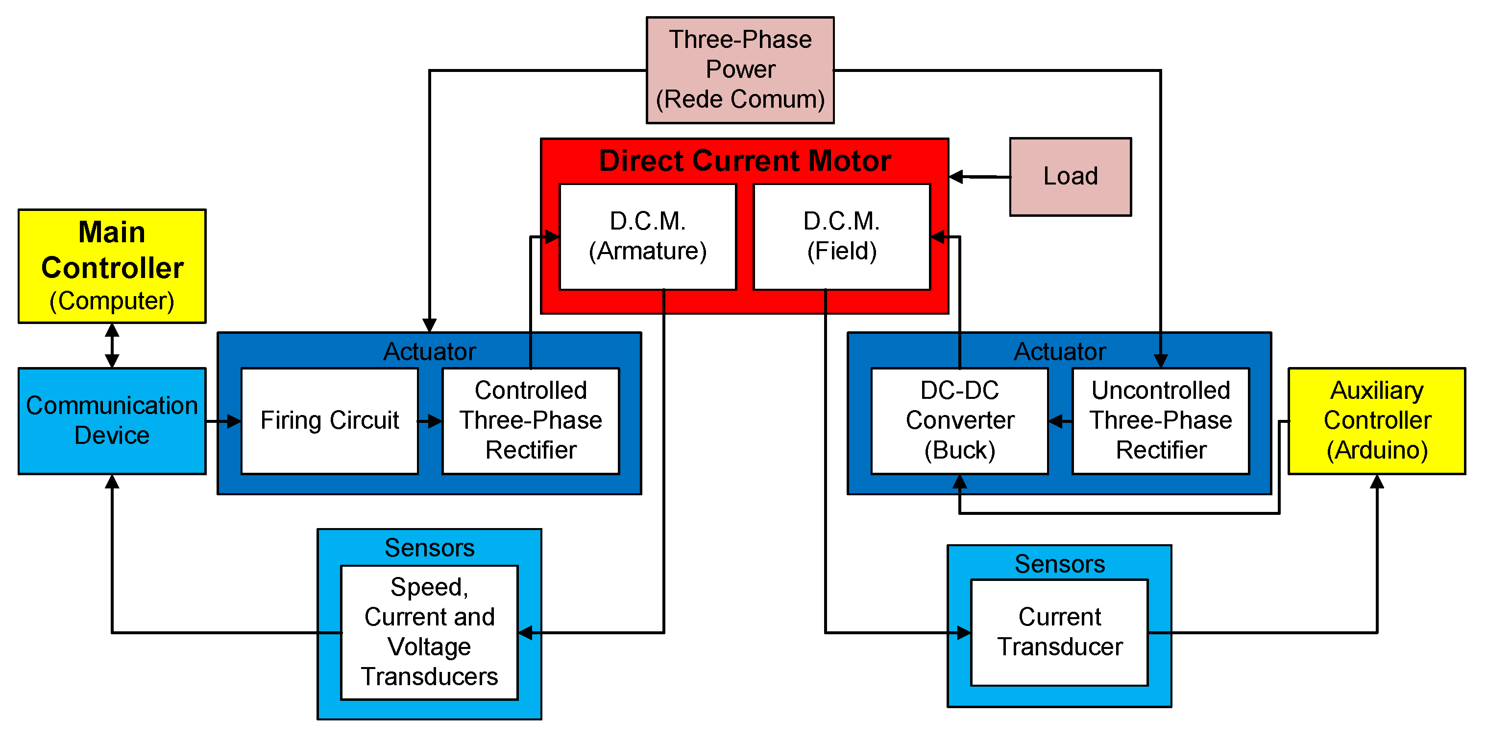
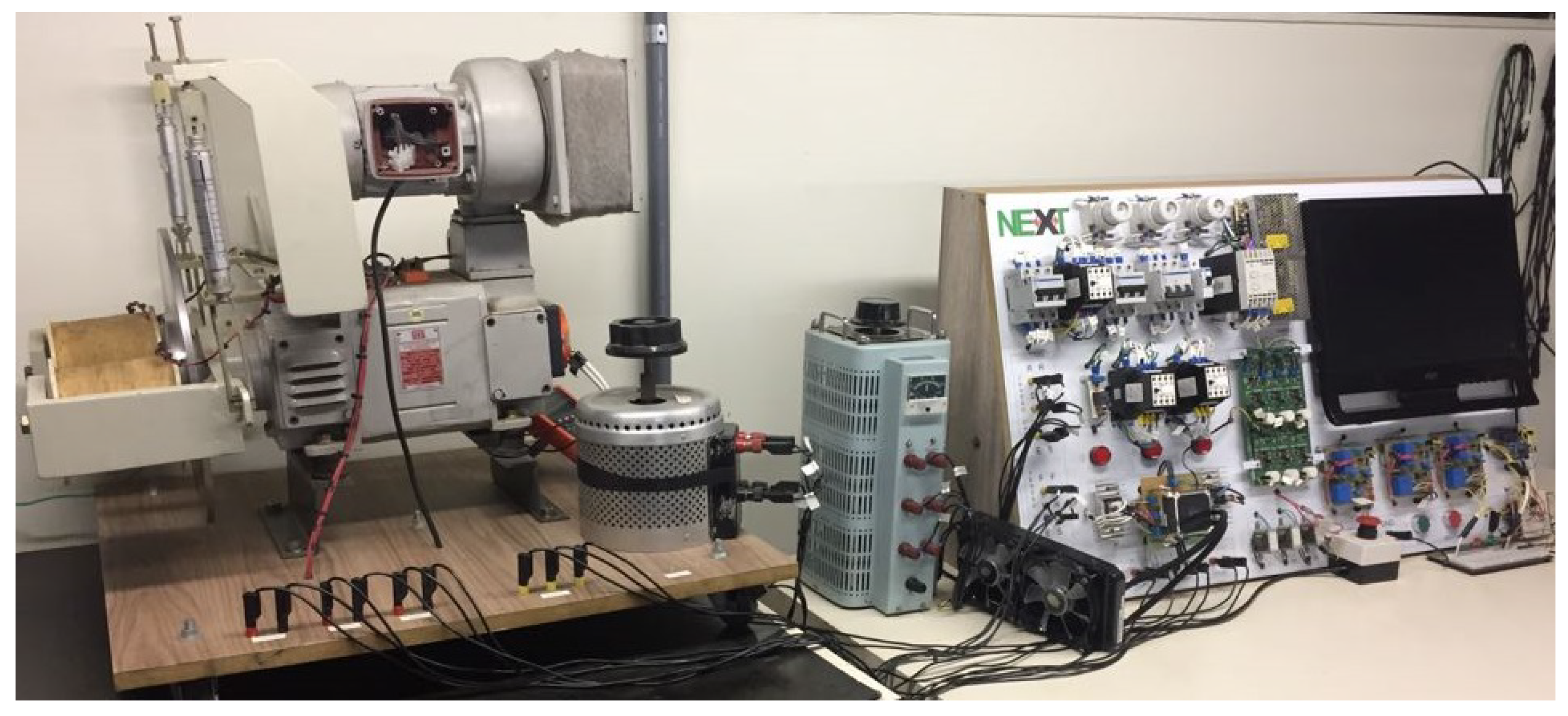
The proposed system is composed of a direct current motor (DC motor) powered by a three-phase fully controlled rectifier (TPFCR). Figure 5 shows the bench with the implemented system, in which the state of the current configuration is the result of the evolution promoted through improvements, substitutions and adjustments made to the bench initially designed and used in the works Dias et al. [21] and Ganzaroli et al. [40].

The main element of the system is the DC motor of independent excitation. Its main electrical characteristics indicated in the nameplate data are: (i) power of 1 kW, (ii) nominal armature voltage 220 V, (iii) nominal current in the armature of 5.5 A, (iv) nominal field voltage of 190 V and (v) nominal field current of 1.15 A. The DC motor has elements associated with its structure and installed by the manufacturer, such as forced ventilation system, electromagnetic brake and tachogenerator coupled to the shaft. 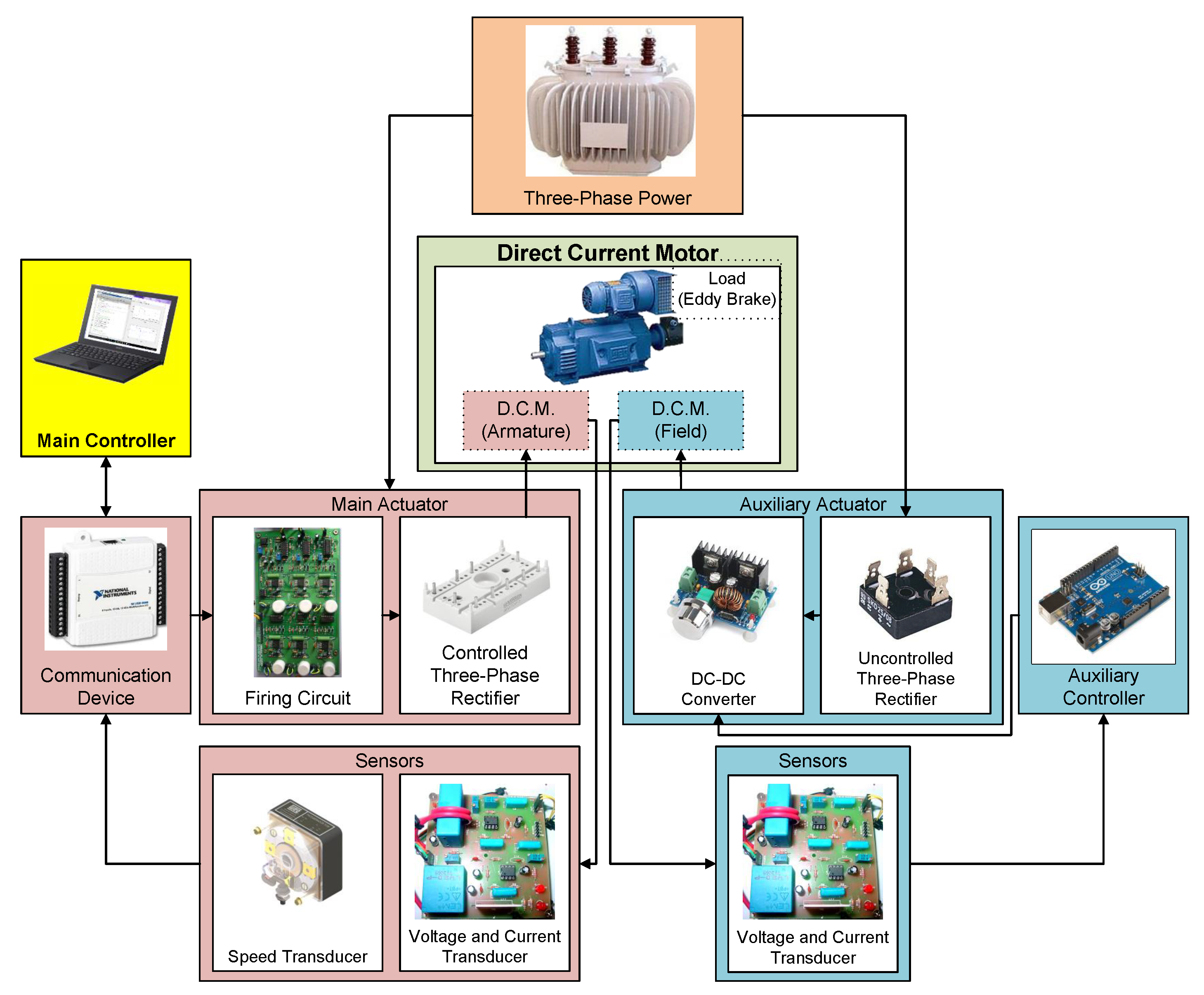Figure 6 shows the diagram of the association between the system components, trigger circuit, devices for communication, measurement and signal conditioning.

Among the possibilities of choosing the different connection configurations, independent excitation was chosen, in order to obtain a relationship between the armature voltage and the speed developed by the DC motor. The field voltage is provided by the auxiliary control system. The field voltage is provided by the auxiliary control system. In this system, the PID control action is calculated by a routine implemented in the development platform that uses the ATmega328P microcontroller. This platform receives the field current signal from the current sensors, calculates the control action and provides as a result the Pulse-width modulation (PWM) voltage signal and applies it to the Buck DC-DC converter. The Buck converter has, at its output, the average voltage value equal or lower than the input voltage, as the control signal applied to its static switch. For this application, the input voltage is generated by the uncontrolled three-phase SKD25/08 rectifier from the Semikron^® manufacturer.

The implementation of the main control action is performed through the armature voltage of the DC motor and is supplied through the fully controlled three-phase rectifier. For this element, the SK70DT16 bridge from the Semikron^® manufacturer was used. This bridge operates with voltages up to 1600 V and a current of 70 A. The generation of pulses and the control of the conduction period of the thyristors are performed by the electronic tripping circuit. This circuit is based on the use of three commercial TCA785, being the IC for each pair of thyristors. The operation of the integrated circuit is based on the application of a continuous voltage signal of low magnitude that proportionally promotes the displacement of the position of pulse generation within the range in which the thyristor is able to conduct.

The use of the TCA785 IC makes the logic that relates the control voltage signal from the circuit $V_c$ and the DC motor armature voltage $V_a$ is reversed. This establishes the relationship between the percentage control action, the control voltage signal from the trigger circuit $V_c$ and the DC motor armature voltage $V_a$: for 0.00% control action, $V_c=4.10$ where V represents $V_a\approx 0$ V; for 100% control action, $V_c=2.7$ where V represents $V_a\approx 230$ V. The speed signal was obtained by the tachogenerator coupled to the DC motor shaft. The voltage × speed ratio was 20 mV/rpm. Considering the possibility of speeds up to 2000 rpm and the specifications of the multifunctional input-output device, the resistive voltage divider was used, converting the value of this ratio to 5 mV/rpm. In addition, the output signal has high frequency noise characteristic of the tachogenerator, requiring the presence of the low-pass filter in order to condition the speed signal and reduce the noise.

The voltage and current signals from the armature circuit, the field circuit and the electromagnetic brake system come from Hall Effect sensors. The sensor used to measure the voltage was LV-25P, with a maximum voltage of 500 V. For the current, the LA-55P was used, which operates with currents of up to 55 A. These elements are associated with signal conditioners represented by the Butterworth filter of second order with active amplifier. The power supply for the electronic circuits was supplied by regulated 5 V and 12 V regulated voltage sources. The interface between the computer and the system was performed by means of the multifunctional input-output device. The USB-6008 from National Instruments^® was used. Among its main features are: (i) bus power supply; (ii) eight analog inputs with acquisition rate up to 10,000 samples/s, resolution up to 12 bits, −10 V to 10 V range with 37.5 mV accuracy; (iii) two analog outputs with an acquisition rate of up to 150 amostras/s, resolution up to 12 bits, 0 V to 5 V range with 7 mV of accuracy and current up to 10 mA; (iv) twelve digital channels configurable as input or output, all with 0 V to 5 V, range, 37.5 mV of accuracy, 5 mV and output current up to 102 mA; and (v) one 32 bit counter channel.

Table 1. Summary of DC motor parameters.

Parameter	Value
Power	1 kW
Nominal armature voltage	220 V
Nominal armature current	5.5 A
Nominal field voltage	190 V
Nominal field current	1.15 A

and

Table 2. Summary of three-phase fully controlled rectifier parameters.

Parameter	Value
Manufacturer	Semikron
Model	SK70DT16
Peak Repetitive Off-State Voltage $\left(V_{DRM}\right)$	1.6 kV
On State RMS Current $\left(I{T}_{RMS}\right)$	68 A
Gate trigger voltage $\left(V_{GT}\right)$	2 V
Gate Trigger Current $\left(I_{GT}\right)$	100 mA

provide a summary of the parameters of the DC motor and the three-phase fully controlled rectifier parameters (TPFCR).

4.2. Optimization Process Applied to the Model

The model used is the result of the identification process performed by the NARMAX method, considering two inputs and three outputs. The process of obtaining the model follows the main steps proposed by [41]: (i) dynamic testing and data collection, (ii) choice of the mathematical representation, (iii) structure selection, (iv) parameter estimation and (v) validation with the system. The dynamic tests were performed by applying the signal characterized basically by the gradual variation, increasing and decreasing at different levels within the voltage range supported by the DC motor.

The signal configuration was established in order to capture the transient behavior from the variations at different levels, the behavior on the permanent regime allowing the signal to remain long enough to stabilize the system response, as well as the various dynamics such as hysteresis through increasing and decreasing variation considering the same voltage levels and dead time, comparing the instant of transitions in the input signal and the output signal. The sampling period was set at $T_s=100$ ms, respecting the Nyquist theorem and the processing time required for the calculation and execution of the control action.

The characteristics of the mathematical representation using the NARMAX model are expressed by: (i) sigmoidal regressors, (ii) two inputs, control voltage and shaft load and (iii) three outputs, speed, armature voltage and armature current. Expressions (21) through (23) present the optimized parameters for defining the structure of the system model; expressions (24) through (30) ) present the optimized system model coefficients for speed outputs; expressions (31) through (37) present the optimized system model coefficients for armature voltage outputs; and expressions (38) through (44) present the optimized system model coefficients for armature current outputs.

Expressions (21) through (44) are values that determine the selection structure and parameters of the NARMAX model, resulting from the heuristic optimization process using genetic algorithm (GA). The implementation of the GA for determining the model parameters was performed considering: (i) initial randomly generated population with 15 individuals, (ii) linear crossover rate $P_{CL}=[90\%;30\%]$, (iii) linear mutation rate $P_{ML}=[30\%;90\%]$. The selection method adopted was the tournament involving four individuals, $\tau =4$ and the stopping criteria were set at 30 generations, $G_{max}=30$ or until obtaining $f\left(x\right)=0$. The uniform mutation operator and the crossover operator with a cutoff point were used. The evaluation function used is given by (45), which is formed by the motor speed IAE${}_{\omega }$ plus the penalties relative to the nominal armature voltage $V_n=230$ V and the peak current In $I_n=38$ A.

$$n_a=\left[\begin{array}{ccc}0& 3& 0\\ 0& 1& 1\\ 0& 1& 2\end{array}\right]$$

(21)

$$n_b=\left[\begin{array}{cc}3& 2\\ 4& 7\\ 2& 0\end{array}\right]$$

(22)

$$n_k=\left[\begin{array}{cc}0& 2\\ 0& 0\\ 0& 0\end{array}\right]$$

(23)

$$P_1=\left[\begin{array}{ccccc}1.29\times {10}^{-3}& 2.27\times {10}^{-3}& -1.66\times {10}^3& -1.25\times {10}^{-1}& -3.86\times {10}^{-1}\\ 1.43\times {10}^{-4}& -6.97\times {10}^{-4}& 1.31\times {10}^{-2}& 1.14& 3.50\\ 2.56\times {10}^{-7}& -3.16\times {10}^{-4}& 3.98\times {10}^{-3}& 3.23\times {10}^{-1}& -1.25\times {10}^1\\ 5.05\times {10}^{-5}& -2.82\times {10}^{-2}& -3.32\times {10}^{-1}& 3.46\times {10}^{-3}& 6.76\times {10}^{-3}\\ 5.07\times {10}^{-5}& -2.79\times {10}^{-2}& 3.36\times {10}^{-1}& -4.59\times {10}^{-2}& 1.64\times {10}^{-2}\end{array}\right]$$

(24)

$$L_1^{\prime }=\left[\begin{array}{ccccc}7.65\times {10}^2& -5.75& 1.19\times {10}^{-1}& 5.95& -3.35\end{array}\right]$$

(25)

$$d_1=\left[\begin{array}{c}1.19\times {10}^3\end{array}\right]$$

(26)

$$Q_1=\left[\begin{array}{ccccc}1.29\times {10}^{-3}& 2.27\times {10}^{-3}& -1.66\times {10}^3& -1.25\times {10}^{-1}& -3.86\times {10}^{-1}\\ 1.43\times {10}^{-4}& -6.97\times {10}^{-4}& 1.31\times {10}^{-2}& 1.14& 3.50\\ 2.56\times {10}^{-7}& -3.16\times {10}^{-4}& 3.98\times {10}^{-3}& 3.23\times {10}^{-1}& -1.25\times {10}^1\\ 5.05\times {10}^{-5}& -2.82\times {10}^{-2}& -3.32\times {10}^{-1}& 3.46\times {10}^{-3}& 6.76\times {10}^{-3}\\ 5.07\times {10}^{-5}& -2.79\times {10}^{-2}& 3.36\times {10}^{-1}& -4.59\times {10}^{-2}& 1.64\times {10}^{-2}\end{array}\right]$$

(27)

$$A_1=\left[\begin{array}{ccccc}-2.65\times {10}^2& 3.78\times {10}^1& -2.53\times {10}^2& 5.83& -6.45\end{array}\right]$$

(28)

$$B_1=\left[\begin{array}{ccccc}-1.42& 1.02& 1.12& 1.61& 1.98\\ 4.78\times {10}^{-1}& 1.96\times {10}^{-1}& -3.42\times {10}^{-1}& -7.71\times {10}^{-1}& 2.96\times {10}^{-1}\\ -3.94\times {10}^{-3}& -2.80\times {10}^{-2}& 5.16\times {10}^{-3}& -2.09\times {10}^{-2}& 6.47\times {10}^{-2}\\ -9.91\times {10}^{-2}& -9.59\times {10}^{-2}& 8.76\times {10}^{-2}& 9.59\times {10}^{-3}& 4.15\times {10}^{-2}\\ 2.14\times {10}^{-1}& -3.09\times {10}^{-1}& -2.04\times {10}^{-1}& -1.67\times {10}^{-1}& -1.22\times {10}^{-1}\end{array}\right]$$

(29)

$$C_1=\left[\begin{array}{ccccc}6.43& -5.12& -5.59& -2.85& -2.75\end{array}\right]$$

(30)

$$P_2=\left[\begin{array}{ccccc}1.29\times {10}^{-3}& 2.27\times {10}^{-3}& -1.66\times {10}^3& -1.25\times {10}^{-1}& -3.86\times {10}^{-1}\\ 1.43\times {10}^{-4}& -6.97\times {10}^{-4}& 1.31\times {10}^{-2}& 1.14& 3.50\\ 2.56\times {10}^{-7}& -3.16\times {10}^{-4}& 3.98\times {10}^{-3}& 3.23\times {10}^{-1}& -1.25\times {10}^1\\ 5.05\times {10}^{-5}& -2.82\times {10}^{-2}& -3.32\times {10}^{-1}& 3.46\times {10}^{-3}& 6.76\times {10}^{-3}\\ 5.07\times {10}^{-5}& -2.79\times {10}^{-2}& 3.36\times {10}^{-1}& -4.59\times {10}^{-2}& 1.64\times {10}^{-2}\end{array}\right]$$

(31)

$$L_2^{\prime }=\left[\begin{array}{ccccc}8.56\times {10}^1& -9.85\times {10}^{-1}& -5.09\times {10}^{-2}& 1.37& -6.58\times {10}^{-1}\end{array}\right]$$

(32)

$$d_2=\left[\begin{array}{c}1.32\times {10}^2\end{array}\right]$$

(33)

$$Q_2=\left[\begin{array}{ccccc}1.29\times {10}^{-3}& 2.27\times {10}^{-3}& -1.66\times {10}^3& -1.25\times {10}^{-1}& -3.86\times {10}^{-1}\\ 1.43\times {10}^{-4}& -6.97\times {10}^{-4}& 1.31\times {10}^{-2}& 1.14& 3.50\\ 2.56\times {10}^{-7}& -3.16\times {10}^{-4}& 3.98\times {10}^{-3}& 3.23\times {10}^{-1}& -1.25\times {10}^1\\ 5.05\times {10}^{-5}& -2.82\times {10}^{-2}& -3.32\times {10}^{-1}& 3.46\times {10}^{-3}& 6.76\times {10}^{-3}\\ 5.07\times {10}^{-5}& -2.79\times {10}^{-2}& 3.36\times {10}^{-1}& -4.59\times {10}^{-2}& 1.64\times {10}^{-2}\end{array}\right]$$

(34)

$$A_2=\left[\begin{array}{ccccc}-5.20& 2.86& -2.39& -3.90& -5.78\end{array}\right]$$

(35)

$$B_2=\left[\begin{array}{ccccc}1.08& -1.25& -1.83\times {10}^{-1}& 3.60\times {10}^{-2}& -8.95\times {10}^{-1}\\ 1.79\times {10}^{-1}& 1.02\times {10}^{-1}& 6.18\times {10}^{-1}& 5.70\times {10}^{-2}& 5.35\times {10}^{-1}\\ 7.80\times {10}^{-2}& -3.83\times {10}^{-2}& -1.11\times {10}^{-1}& -1.00\times {10}^{-1}& -7.32\times {10}^{-2}\\ 4.17\times {10}^{-2}& 1.50\times {10}^{-1}& -4.63\times {10}^{-2}& 1.41\times {10}^{-1}& 1.46\times {10}^{-1}\\ -2.76\times {10}^{-1}& 7.17\times {10}^{-2}& -2.87\times {10}^{-1}& -1.58\times {10}^{-1}& -1.07\times {10}^{-1}\end{array}\right]$$

(36)

$$C_2=\left[\begin{array}{ccccc}-6.25& 1.77& 1.46& -1.24& -1.93\end{array}\right]$$

(37)

$$P_3=\left[\begin{array}{ccccc}1.29\times {10}^{-3}& 2.27\times {10}^{-3}& -1.66\times {10}^3& -1.25\times {10}^{-1}& -3.86\times {10}^{-1}\\ 1.43\times {10}^{-4}& -6.97\times {10}^{-4}& 1.31\times {10}^{-2}& 1.14& 3.50\\ 2.56\times {10}^{-7}& -3.16\times {10}^{-4}& 3.98\times {10}^{-3}& 3.23\times {10}^{-1}& -1.25\times {10}^1\\ 5.05\times {10}^{-5}& -2.82\times {10}^{-2}& -3.32\times {10}^{-1}& 3.46\times {10}^{-3}& 6.76\times {10}^{-3}\\ 5.07\times {10}^{-5}& -2.79\times {10}^{-2}& 3.36\times {10}^{-1}& -4.59\times {10}^{-2}& 1.64\times {10}^{-2}\end{array}\right]$$

(38)

$$L_3^{\prime }=\left[\begin{array}{ccccc}2.73\times {10}^{-1}& -5.22\times {10}^{-1}& 3.32\times {10}^{-2}& 1.51\times {10}^{-1}& -1.38\times {10}^{-1}\end{array}\right]$$

(39)

$$d_3=\left[\begin{array}{c}3.03\end{array}\right]$$

(40)

$$Q_3=\left[\begin{array}{ccccc}1.29\times {10}^{-3}& 2.27\times {10}^{-3}& -1.66\times {10}^3& -1.25\times {10}^{-1}& -3.86\times {10}^{-1}\\ 1.43\times {10}^{-4}& -6.97\times {10}^{-4}& 1.31\times {10}^{-2}& 1.14& 3.50\\ 2.56\times {10}^{-7}& -3.16\times {10}^{-4}& 3.98\times {10}^{-3}& 3.23\times {10}^{-1}& -1.25\times {10}^1\\ 5.05\times {10}^{-5}& -2.82\times {10}^{-2}& -3.32\times {10}^{-1}& 3.46\times {10}^{-3}& 6.76\times {10}^{-3}\\ 5.07\times {10}^{-5}& -2.79\times {10}^{-2}& 3.36\times {10}^{-1}& -4.59\times {10}^{-2}& 1.64\times {10}^{-2}\end{array}\right]$$

(41)

$$A_3=\left[\begin{array}{ccccc}1.12& -1.52\times {10}^{-1}& 3.47& -9.41& 3.72\end{array}\right]$$

(42)

$$B_3=\left[\begin{array}{ccccc}-1.72& 1.68& -1.80& -1.03& 4.55\times {10}^{-1}\\ 5.24\times {10}^{-1}& -5.60\times {10}^{-1}& -1.80\times {10}^{-1}& -8.91\times {10}^{-3}& -5.67\times {10}^{-2}\\ -6.81\times {10}^{-2}& -9.69\times {10}^{-2}& 1.02\times {10}^{-1}& 6.90\times {10}^{-2}& -1.06\times {10}^{-1}\\ 7.22\times {10}^{-2}& -7.88\times {10}^{-2}& -1.74\times {10}^{-1}& -1.06\times {10}^{-1}& -1.63\times {10}^{-1}\\ 1.85\times {10}^{-1}& 4.36\times {10}^{-1}& 8.87\times {10}^{-2}& -3.01\times {10}^{-1}& -2.29\times {10}^{-1}\end{array}\right]$$

(43)

$$C_3=\left[\begin{array}{ccccc}5.06& -2.61& 4.48& 7.06\times {10}^{-1}& -3.70\times {10}^{-1}\end{array}\right]$$

(44)

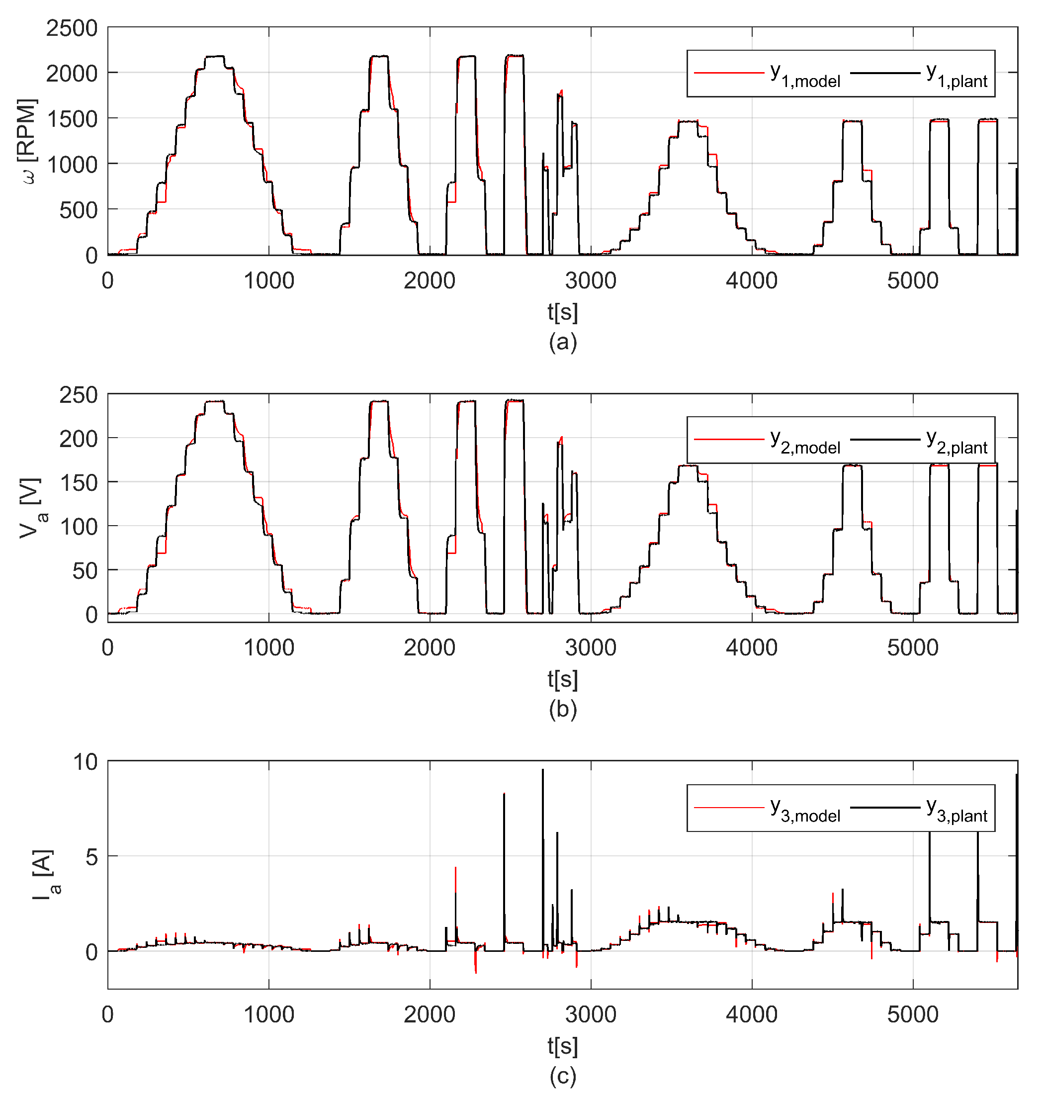
In the validation stage of the NARMAX model, the result generated by the model was compared with the signals obtained from the real system, Figure 5, considering the application of the same input signal to the model and for the plant with and without the presence of load. To evaluate the quality of the model, considering the existence of three outputs, different weights were established according to the relevance of each signal to the work. The weights adopted are: (i) 0.70 for approximation of the motor speed signal $\omega$, (ii) 0.20 for approximation of the armature voltage signal $V_a$ and (iii) 0.10 for approximation of the armature current signal $I_a$. The output signals of the real × model system are shown in Figure 7. The individual approximation rate for each output is 91.12% for the speed signal, 91.69% for the armature voltage signal and 86.04% for the armature current signal. After the assignment of the weights, the overall model evaluation criterion rate was 90.16%.

Figure 7 shows the unloaded tests in the range $[0;3.0\times {10}^3]$ and the loaded tests in the range $[3.0\times {10}^3;5.650\times {10}^3]$. The implementation of the load is identified in the response of the system through reduced speed levels and increased armature current levels when compared to the test without the presence of the load, despite the reference signal being the same for both tests. This behavior is characteristic of the DC motor operating in open loop, i.e., in the absence of the control system.

4.3. Applying the Optimization Process to Controllers

The tuning of the controllers is performed, as well as the optimization of the model parameters by the heuristic optimization method genetic algorithm (GA). The implementation of the GA for tuning the parameters of all the controllers studied was established based on the considerations: (i) initial randomly generated population with 50 individuals, (ii) linear crossover rate $P_{CL}=[90\%;30\%]$, (iii) linear mutation rate $P_{ML}=[30\%;90\%]$. The selection method adopted was the tournament involving five individuals, $\tau =5$ and the stopping criteria were set at 250 generations, $G_{max}=250$ or until obtaining $f\left(x\right)=0$. The Non-Uniform Mutation operator and the Simple Crossover operator were used. The evaluation function used is given by (45), which is formed by the IAE${}_{\omega }$ of engine speed plus penalties related to the nominal armature voltage $V_n=230$ V and the peak current $I_n=38$ A.

$$f\left(x\right)=IA{E}_{\omega }+P_V+P_I$$

(45)

Heuristic optimization searches for the best solution to the problem within the search space $\Omega$. The definition of $\Omega$ is directly related to the speed of convergence of the algorithm and thus, specific limits were established for the parameters of each controller based on a priori knowledge of the system. The proposed simulator used in the optimization process represents different scenarios, due to different setpoints, different dynamics and the insertion or removal of loads. This simulator allows the optimization to be performed considering the main characteristics and dynamics of the system. In this way, the optimized parameters of the various controllers, take into account the different dynamics for the different operating points.

4.3.1. Tuning of the PID Controller

The tuning of the PID controller sought to optimize the parameters in the sets referring to the search space $\Omega$ of each constant: (i) proportional constant $\{K_p\in \mathbb{R}|1\times {10}^{-6}\le K_p\le 100\}$, (ii) integral constant $\{K_i\in \mathbb{R}|0\le K_i\le 100\}$ and (iii) derivative constant $\{K_d\in \mathbb{R}|0\le K_d\le 100\}$.

Table 3. Optimized parameters for tuning the PID controller.

Parameters	${\mathit{K}}_{\mathit{p}}$	${\mathit{K}}_{\mathit{i}}$	${\mathit{K}}_{\mathit{d}}$
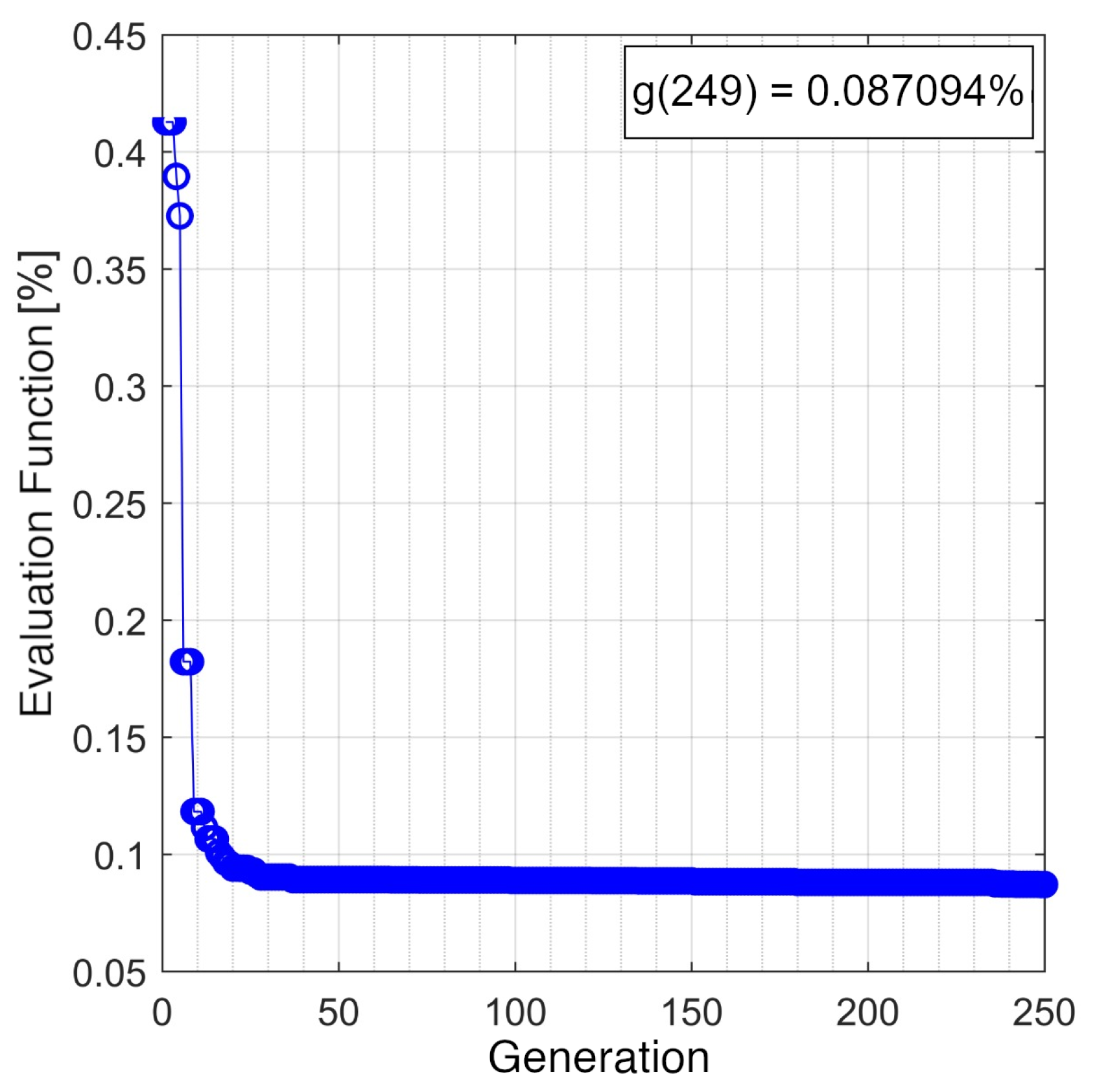
Values	0.0311	$1.37\times {10}^{-7}$	0.0112

provides the optimized values for the tuning parameters of the PID controller and Figure 8 presents the performance of the GA over the generations. It can be seen that the best individual was obtained in generation 249 with the value of $f\left(x\right)=0.087094\%$.

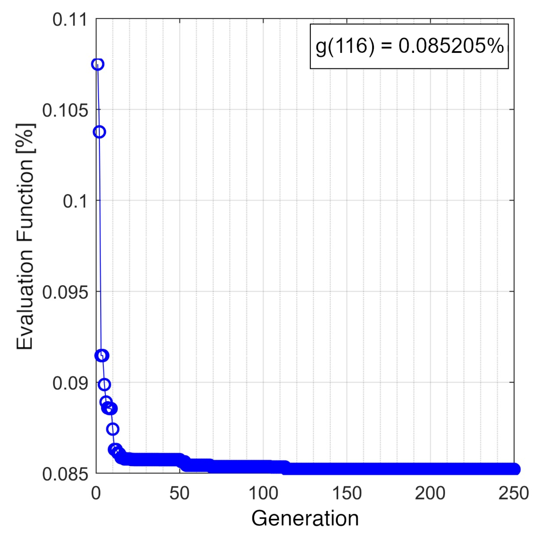
4.3.2. Tuning of the Practical Nonlinear Predictive Controller

The PNMPC controller was optimized by considering the parameters bounded by their respective search spaces $\Omega$: (i) prediction horizon: $\{N_y\in \mathbb{N}|1\le N_y\le 50\}$, (ii) control horizon: $\{N_u\in \mathbb{N}|1\le N_u\le N_y\}$, (iii) damping rate of the reference signal: $\{{\alpha }_r\in \mathbb{R}|0.00\le {\alpha }_r\le 1.00\}$, (iv) damping rate of the control action: $\{\lambda \in \mathbb{R}|0.00\le \lambda \le 1.00\times {10}^4\}$, (v) damping rate of nonlinearity of the $G_{PNMPC}$ matrix: $\{{\gamma }_G\in \mathbb{R}|0.00\le {\gamma }_G\le 1.00\}$ and (vi) variation for linearization at each sampling instant: $\{ϵ\in \mathbb{R}|-1.00\times {10}^6\le ϵ<-1.00;1.00<ϵ\le 1.00\times {10}^6\}$. The optimized parameters of the PNMPC controller are arranged in

Table 4. Optimized parameters for the Practical Nonlinear Predictive Controller.

Parameters	${\mathit{N}}_{\mathit{y}}$	${\mathit{N}}_{\mathit{u}}$	${\mathit{\alpha }}_{\mathit{r}}$	$\mathit{\lambda }$	${\mathit{\gamma }}_{\mathit{G}}$	$\mathit{ϵ}$
Values	10	1	$1.61\times {10}^{-4}$	$3.28\times {10}^{-4}$	$3.00\times {10}^{-4}$	$5.02\times {10}^2$

, and Figure 9 shows the performance of the GA over the generations in the optimization process, in which it is observed that the best individual was obtained in generation 116 with the value of $f\left(x\right)=0.085205\%$.

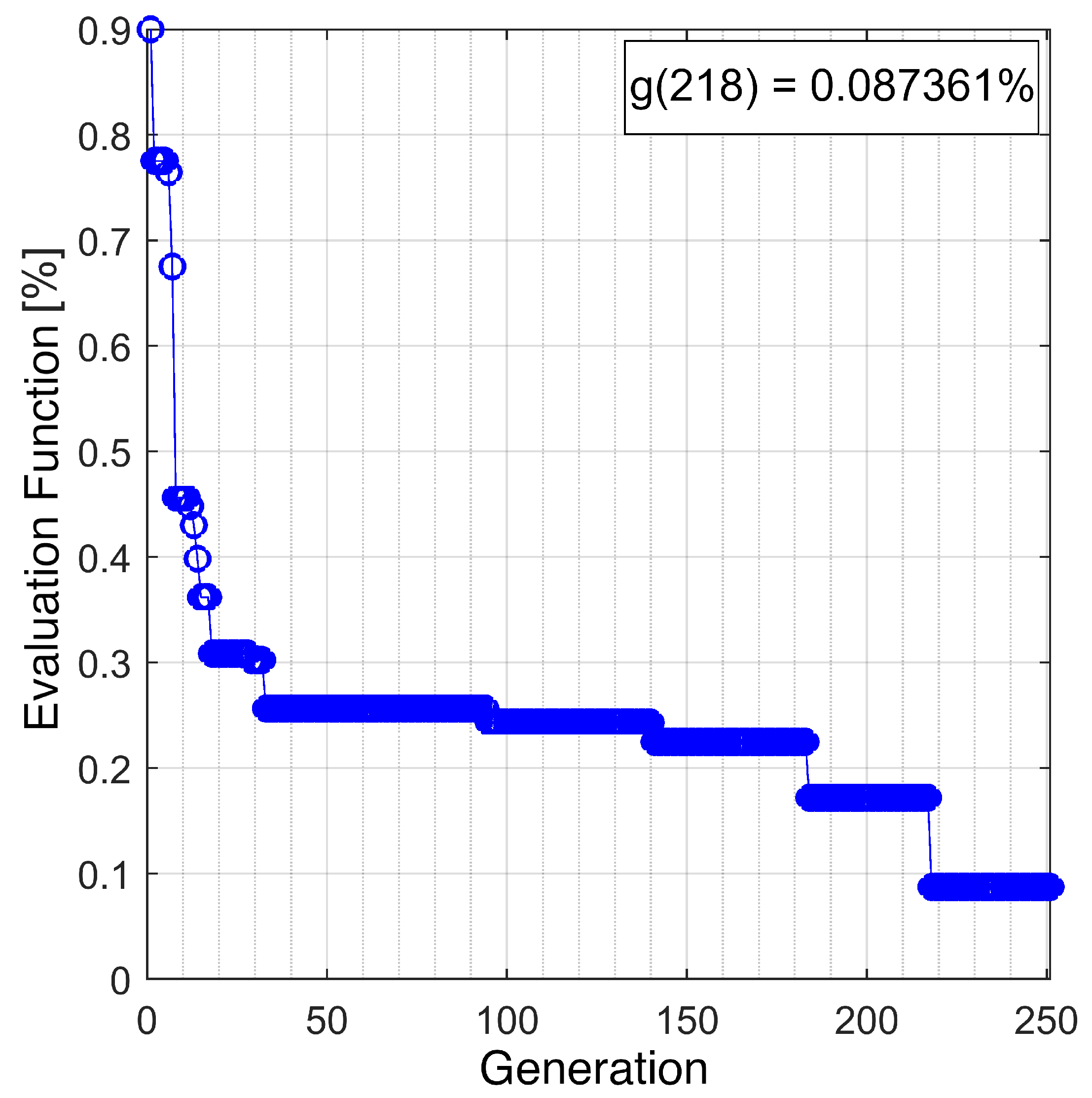
4.3.3. Tuning of the Fuzzy Controller

The optimization of the membership functions of the fuzzy controller resulted in the values of the limits shown in

Table 5. Limits of the membership functions for the input and output variables of the fuzzy controller.

Linguistic Variable—Error
$MF1$	$MF2$	$MF3$	$MF4$	$MF5$
$2.06\times {10}^2$	$1.23\times {10}^2$	$4\times {10}^{-1}$	$9.74\times {10}^1$	$-2.50\times {10}^3$
$8.42\times {10}^2$	$1.59\times {10}^2$	$2.32\times {10}^1$	$1.79\times {10}^3$	$7.05\times {10}^1$
$1.84\times {10}^3$	$1.86\times {10}^2$	$6.03\times {10}^1$	$2.50\times {10}^3$	$5.97\times {10}^2$
$2.50\times {10}^3$	$2.22\times {10}^3$	$2.11\times {10}^3$	$2.50\times {10}^3$	$8.16\times {10}^2$
Linguistic Variable—Error Variation
$3.65\times {10}^2$	$4.69\times {10}^1$	$-2.76\times {10}^2$	$-5.13$	$-4.16\times {10}^2$
$8.48\times {10}^2$	$1.84\times {10}^3$	$4.55\times {10}^1$	$4.09\times {10}^2$	$4.47\times {10}^2$
$1.43\times {10}^3$	$2.35\times {10}^3$	$1.47\times {10}^2$	$2.50\times {10}^3$	$4.49\times {10}^2$
$2.50\times {10}^3$	$2.35\times {10}^3$	$2.59\times {10}^2$	$2.50\times {10}^3$	$2.50\times {10}^3$
Linguistic Variable—Control Action
$4.99\times {10}^1$	$5\times {10}^1$	$5\times {10}^1$	$5.01\times {10}^1$	$4.29\times {10}^1$
$5.83\times {10}^1$	$7.28\times {10}^1$	$5.01\times {10}^1$	$7.73\times {10}^1$	$4.49\times {10}^1$
$6.39\times {10}^1$	$9.59\times {10}^1$	$5.08\times {10}^1$	$7.74\times {10}^1$	$5\times {10}^1$
$8.10\times {10}^1$	$1\times {10}^2$	$5.44\times {10}^1$	$1\times {10}^2$	$5\times {10}^1$

. The choice of trapezoidal shape is a consequence of the inability of the controller to meet the requirements of the output signal specification with triangular functions. The membership functions, $MF1$ to $MF5$, represent the degree of truth of the variables Error and Error Variation, considering their universes of discourse.

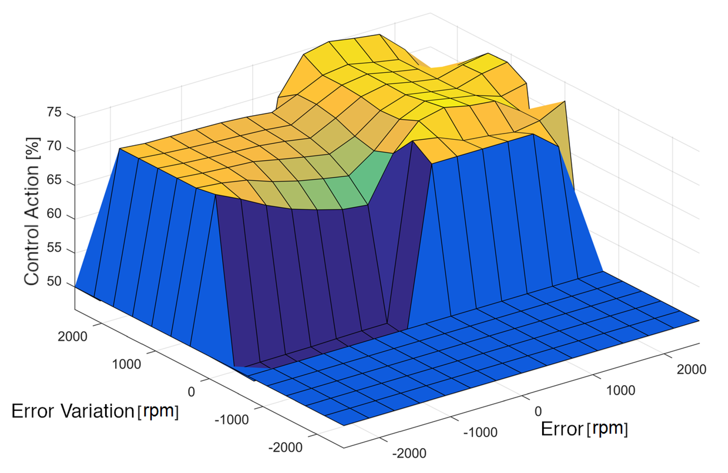
Figure 10 shows the performance of the GA over the generations in the process of fuzzy controller optimization. It can be seen that the best individual was obtained in generation 218 with the value of $f\left(x\right)=0.087361\%$. The fuzzy response surface, shown in Figure 11, indicates sharp transitions resulting from the irregular shapes obtained for the membership functions.

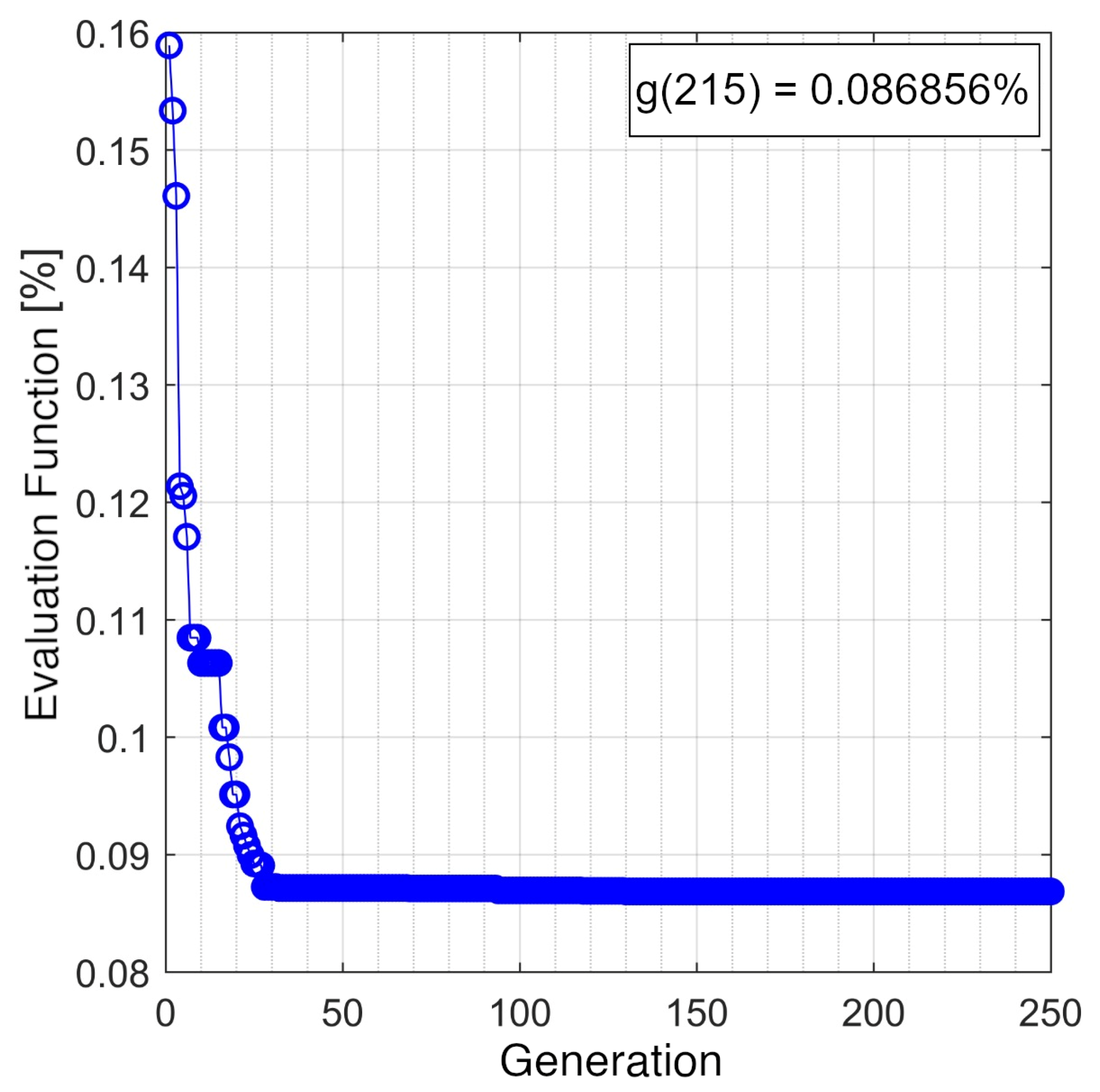
4.3.4. Tuning of the Discrete Sliding Mode Controller

The DSMC optimization considers the parameters: (i) B, which is associated with the second order sliding function, (ii) M, which determines the amplitude of the signal function and (iii) C, which enforces the dynamic behavior of the output variable. In the optimization, all parameters are bounded by their respective search spaces as: $\{B,M,C\in \mathbb{R}|0\le B,M,C\le 1\}$, in which the values optimized by the GA are arranged in

Table 6. Optimized parameters for tuning the sliding mode control.

Parameters	B	M	C
Values	0.00001	0.1	0.79

. Figure 12 shows the performance of the GA over the generations, in which the best individual was obtained in generation 215 with the value of $f\left(x\right)=0.086856\%$.

4.4. Comparison of Control Results from Simulations and Practical Tests

The individual performance of the PID, DSMC, Fuzzy and PNMPC controllers after having their parameters tuned is verified through simulations and test executions on the DC motor system. For each control technique presented, three tests were performed: (i) analysis of the transient response through the settling time and the possible occurrence of overshoot, (ii) analysis of the permanent response of the system at different levels of the reference signal and (iii) analysis of the response of the control system to disturbances in the output variable through load insertion and removal while keeping the reference speed signal constant.

4.4.1. Test with Application of Step Signal

In the first test, the step signal with amplitude 1000 rpm for the reference speed was used. The total duration time was 30 s. In this test, no load was applied to the DC motor.

Table 7. Speed signal of the analyzed controllers considering the application of step signal.

Controller	${\mathit{IAE}}_{\mathit{\omega }}$	${\mathit{T}}_{\mathit{r}}\left[\mathit{s}\right]$	${\mathit{T}}_{\mathit{s}}\left[\mathit{s}\right]$
PID	2.81%	3.10	5.50
PNMPC	2.31%	0.3	1.5
Fuzzy	2.01%	0.5	1.10
DSMC	3.43%	0.5	2.5

provides the values of $IA{E}_{\omega }$, rise time $T_r$ and settling time $T_s$ for each control technique. The speed and armature voltage signals regarding the application of each controller are presented in Figure 13.

In this first test, the four controllers present satisfactory results, but the Fuzzy controller presents lower values of $IA{E}_{\omega }$ and $T_s$, while the PNMPC obtained the best $T_r$.

4.4.2. Test with Varying Amplitude of the Reference Signal

For the second test, the reference signal with different amplitude values was applied with: (i) $0\le t<30$ s and speed reference at 500 rpm, (ii) $30s\le t<60$ s and speed reference at 1700 rpm, (iii) 60 s $\le t<120$ s and speed reference at 1000 rpm and (iv) $120s\le t\le 150$ s and speed reference speed reference at 1500 rpm. No load was applied to the DC motor in this test.

Table 8. System response with application of the reference signal with amplitude variation.

Controller	${\mathit{IAE}}_{\mathit{\omega }}$	Time Interval[s]	${\mathit{T}}_{\mathit{r}}\left[\mathit{s}\right]$	${\mathit{T}}_{\mathit{d}}\left[\mathit{s}\right]$	${\mathit{T}}_{\mathit{s}}\left[\mathit{s}\right]$
PID	3.78%	$0-30$	0.18	-	6.4
		30–60	3.2	-	4.1
		60–120	-	5	9
		120–150	2	-	5
PNMPC	3.34%	0–30	0.3	-	5
		30–60	2.5	-	2.5
		60–120	-	5	9
		120–150	1	-	4
Fuzzy	3.51%	0–30	0.17	-	5.58
		30–60	1.24	-	2.56
		60–120	-	5	9
		120–150	1.32	-	1.75
DSMC	3.89%	0–30	0.1	-	7
		30–60	0.4	-	4
		60–120	-	5	9
		120–150	1.5	-	4

provides the values of $IA{E}_{\omega }$, $T_r$ and $T_s$ for each control technique. The speed and armature voltage signals referring to the application of each controller are presented in Figure 14.

In this second test, PNMPC presented the best $IA{E}_{\omega }$ among the control techniques used. As for the values of $T_r$ and $T_s$, the controllers presented similarity in their results. It can be observed that $T_d$ had a high value for the four techniques. This occurs due to the inertia of the DC motor. Therefore, these values are normal for any control technique.

4.4.3. Load Application Test

In the third test, the reference speed was set at 1000 rpm and the load insertion occurred between $t=30$ s and $t=60$ s.

Table 9. System response with load application.

Controller	${\mathit{IAE}}_{\mathit{\omega }}$	${\mathit{T}}_{\mathit{r}}\left[\mathit{s}\right]$	${\mathit{T}}_{\mathit{s}}\left[\mathit{s}\right]$	${\mathit{T}}_{\mathbf{eic}}\left[\mathit{s}\right]$	${\mathit{T}}_{\mathbf{erc}}\left[\mathit{s}\right]$
PID	1.76%	0.56	5.5	3.2	4
PNMPC	1.41%	0.4	5	2	4
Fuzzy	1.55%	0.55	5	3	4
DSMC	2.25%	0.2	6	3	4

provides the values of $IA{E}_{\omega }$, $T_r$ and $T_s$ for each control technique. The speed and armature voltage signals referring to the application of each controller are presented in Figure 15.

It can be seen from this test that the DSMC controller obtains the lowest $T_r$ and equal value for load removal stabilization time $T_{erc}$, while the PNMPC controller obtained better values of $IA{E}_{\omega }$ and load insertion stabilization time $T_{eic}$.

4.5. Discussion

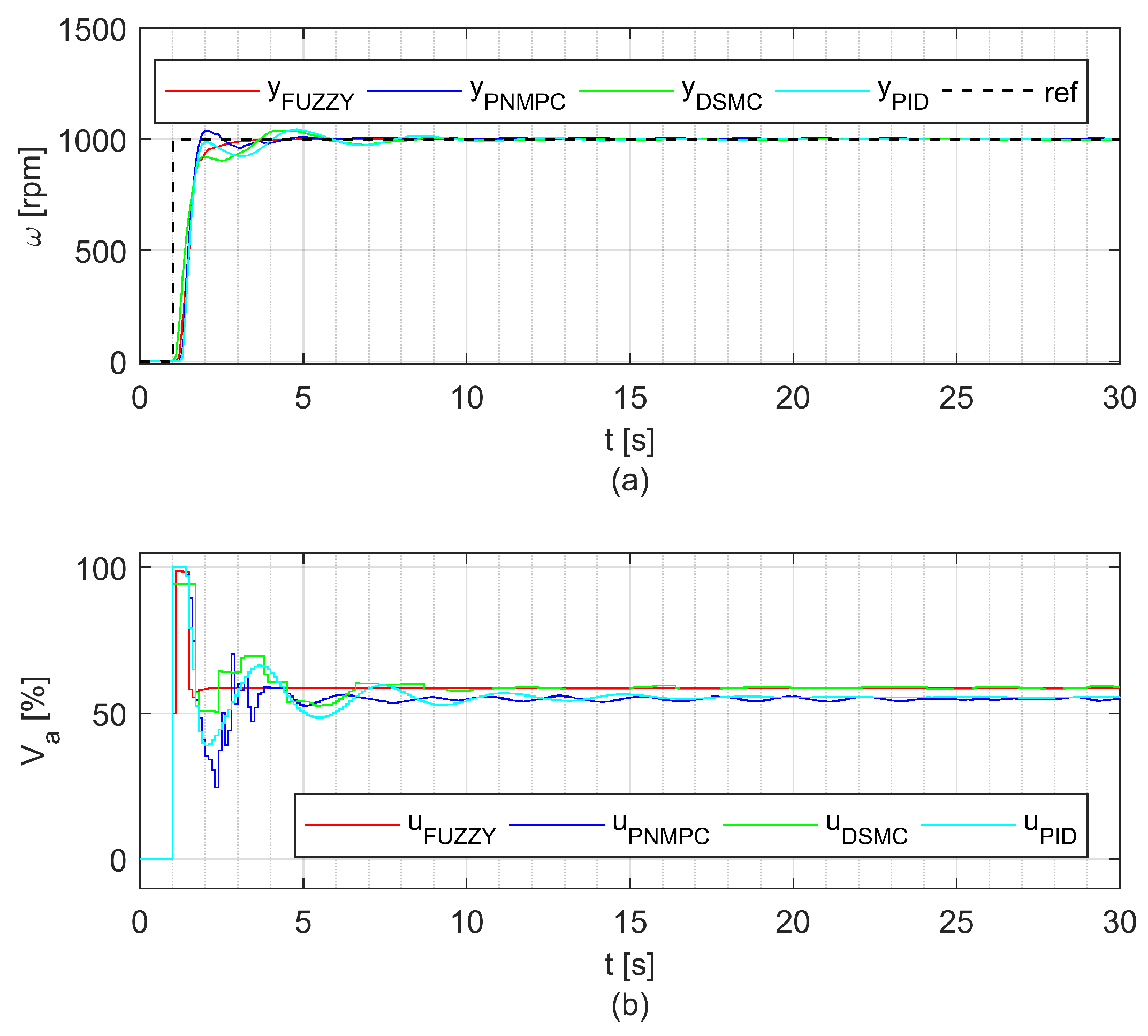
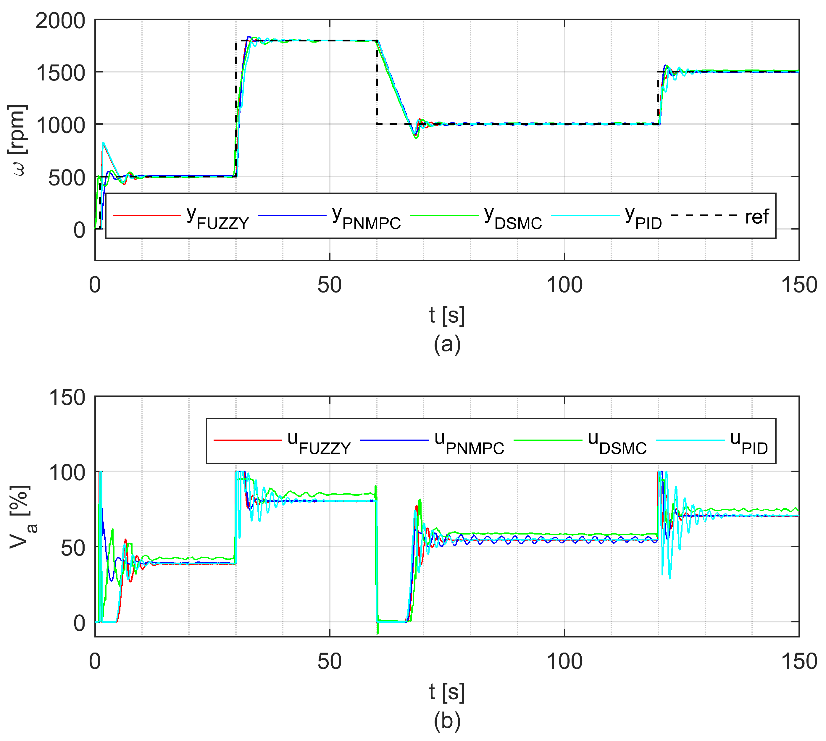
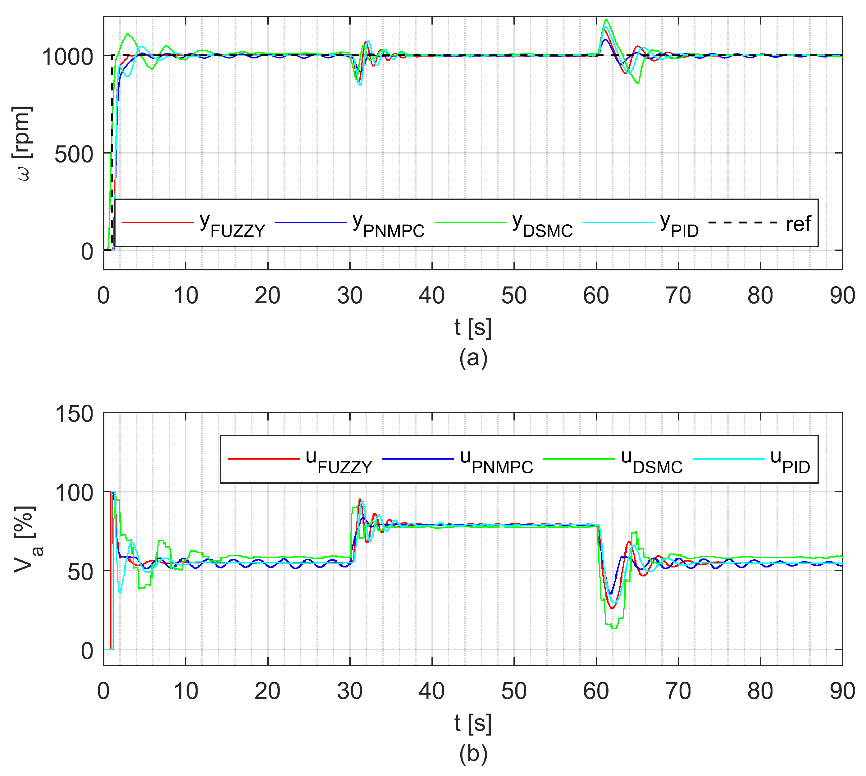
In the comparison between the four control techniques: (i) PID, (ii) PNMPC, (iii) Fuzzy and (iv) DSMC, we presented the characteristics in the performance of each of the controllers. The results indicate the expected performance for the controllers, low $IAE$ values, rise time $Tr$, settling time $T_s$, load insertion stabilization time $T_{eic}$ and load removal stabilization time $T_{erc}$.

In general, the controllers showed responses with similar dynamics, but from an implementation point of view, each technique has its own particularities: the PID control stood out for its simplicity in implementation; however, despite having wide applications, it has difficulties in situations of nonlinearities and noise. The PNMPC, despite being extremely efficient in nonlinear plants, is extremely dependent on the model and requires high computational effort, since it needs to run the model in parallel with the control. The Fuzzy controller showed low mathematical dependence, requiring only the knowledge of the system. The DSMC, despite using mathematical analysis, stands out in design for its robustness, presenting itself as insensitive to the parametric uncertainties of the plant.

The PID control showed a significant trade-off relationship between the spare signal value and the rise time, $Tr$, as verified by Dubey et al. [42]. This relationship shows that lower rise values are related to an increase in the overshoot. The responses of the Fuzzy, PNMPC controllers confirmed the direct model independence mentioned in the works of Kovacic and Bogdan [43] and Yang et al. [44]. The dynamic complexities associated with the control of nonlinear systems are generally factors that make it difficult to tune the PID control parameters. Thus, differently from the methodology of linearization of the plant for tuning these parameters, proposed by authors such as Wang [45], Lan and Woo [46] and Iplikci [47], the use of genetic algorithms allowed the results of PID control to be close to the other techniques studied. The PID controller is based on a linear control technique. To adjust the parameters of this controller in a non-linear system, it is necessary to consider several operating points. However, the optimized values obtained for these parameters use the proposed simulator, which considers several scenarios with different dynamics. Thus, it is expected that this controller can present satisfactory performance even though the plant is non-linear.

For the implementation of the PID control, an anti wind-up mechanism was used. This was necessary because the control action reached its maximum limit, remaining this value independent of the process output variable. Thus, if this mechanism was not implemented, the error would continue to be integrated and the integral term would become very large, which would promote a slow correction of the output variable.

In this way, this work contributes to the gathering and comparison of different control techniques applied to the same plant with nonlinear characteristics. These techniques have their tuning parameters obtained from the optimization by genetic algorithms. Since this is a practical implementation, it is worth mentioning the obstacles encountered in the construction and configuration of the system. During the execution of the work, changes in the plant were necessary, such as the implementation of field current control, in order to avoid variations in the armature voltage due to electromagnetic interactions. The switching of the converters inserted electrical and electromagnetic noise in the system, making it difficult to read the variables. To solve the problem, filters and shielded cables were installed for conditioning of the measurement of voltage, current and motor speed.

It was observed that the motor temperature has a direct influence on its performance, interfering with the output speed. Even with forced ventilation, periods of operation with prolonged machine running time can cause disturbances in the system. The three-phase converter also received ventilation, in order to provide more stability in the armature supply. The tripping circuit of the three-phase rectifier had ceramic capacitors replaced by polyester capacitors, for being more resistant to thermal alterations.

In the proposal of this work, since the system is composed of motor, converter, trigger circuit, acquisition board and others, it is necessary to represent all these elements in the modeling. As the PNMPC uses the model to calculate its control action, the closer the model is to the real system, the better results will be extracted from this controller. The approximation of the model has a direct effect on the controller tuning, enabling the genetic algorithm to find values for the controller parameters that have $IAE$ and acceptable dynamic behavior.

It was observed that operating under different conditions, the four controllers present similar behavior, in which both achieve satisfactory results. Despite having met the desired results, there is still to explore such as: (i) embed the controllers on the bench, eliminating the use of a computer, (ii) perform the system modeling by using other methods such as neural networks, (iii) replace the three-phase fully controlled rectifier by a dual converter, enabling reversal in the direction of rotation of the motor and (iv) replace the AC-DC converter by a DC-DC converter.

For the speed control methodology adopted, changing the armature voltage and keeping the field constant, it is essential that the field exists before the application of the armature voltage. Hence, it is necessary that the electric control logic does not allow the existence of armature voltage without the presence of a magnetic field because if this condition is not met, there will be increasing acceleration of the rotor until the armature winding breaks, and the mechanical components of the motor may be compromised.

5. Conclusions

This work carried out the implementation, analysis and comparison of the control techniques: (i) PID, (ii) PNMPC, (iii) Fuzzy and (iv) DSMC applied to the DC motor speed control with independent excitation and driven by a three-phase fully controlled rectifier of six pulses. In order to compare the four controllers, similar working conditions were sought, such as: same system, same model, same controller tuning and same performance analysis method.

The methodology presented the design of the bench, the model of the real system using the system identification method, and the adjustments of the controllers’ parameters using an optimization process. For the tuning of the controllers, the genetic algorithm was used. A detailed analysis of the PID, PNMPC, Fuzzy and DSMC controllers was performed, in which three tests were presented: (i) test with fixed speed reference and without load insertion in the motor, (ii) test with variable amplitude speed reference and without load insertion in the motor and (iii) test with fixed speed reference and load insertion and removal in the motor. The verification of the controllers’ efficiency used the $IAE$ values, settling time $T_s$, rise time $T_r$, fall time $Td$, insertion stabilization time $T_{eic}$ and load removal stabilization time $T_{erc}$.

In the comparisons between the techniques, the characteristics and performance when executed under similar conditions were highlighted, presenting the robustness of each control technique when acting on the proposed non-linear system. Thus, it is concluded that the controllers tuned by genetic algorithm, applied to the speed control of DC motor driven by three-phase fully controlled rectifier present satisfactory results. However, the PNMPC controller, when compared to other control techniques, presents better performance. Regarding the robustness and precision of the techniques, even operating with a nonlinear system, it obtained desired results when: (i) in the transient regime time, (ii) in the overspeed and (iii) in the integral of the absolute error between the requested reference and the speed developed by the motor.

References

1. Dorf, R.; Bishop, R. Modern Control Systems, 13th ed.; Pearson Education Limited: London, UK, 2016. [Google Scholar]
2. Paraskevopoulos, P.N. Modern Control Engineering; CRC Press: Boca Raton, FL, USA, 2017. [Google Scholar]
3. Nise, N.S. Control Systems Engineering; John Wiley & Sons: Hoboken, NJ, USA, 2020. [Google Scholar]
4. Airikka, P. Advanced control methods for industrial process control. Comput. Control. Eng. 2004, 15, 18–23. [Google Scholar] [CrossRef]
5. Rodríguez, J.; Pontt, J.; Silva, C.; Cortes, P.; Amman, U.; Rees, S. Predictive current control of a voltage source inverter. In Proceedings of the 2004 IEEE 35th Annual Power Electronics Specialists Conference (IEEE Cat. No. 04CH37551), Aachen, Germany, 20–25 June 2004; Volume 3, pp. 2192–2196. [Google Scholar]
6. Ma, Y.; Borrelli, F.; Hencey, B.; Coffey, B.; Bengea, S.; Haves, P. Model predictive control for the operation of building cooling systems. IEEE Trans. Control. Syst. Technol. 2011, 20, 796–803. [Google Scholar]
7. Khatun, P.; Bingham, C.M.; Schofield, N.; Mellor, P. Application of fuzzy control algorithms for electric vehicle antilock braking/traction control systems. IEEE Trans. Veh. Technol. 2003, 52, 1356–1364. [Google Scholar] [CrossRef]
8. Cupertino, F.; Giordano, V.; Naso, D.; Delfine, L. Fuzzy control of a mobile robot. IEEE Robot. Autom. Mag. 2006, 13, 74–81. [Google Scholar]
9. Camboim, W.; da Silva, S.A.; Gomes, H.P. Application of Fuzzy techniques to control pressure in water supply systems. Eng. Sanit. Ambient. 2014, 19, 67–77. [Google Scholar] [CrossRef] [Green Version]
10. Utkin, V.I. Sliding mode control design principles and applications to electric drives. IEEE Trans. Ind. Electron. 1993, 40, 23–36. [Google Scholar] [CrossRef] [Green Version]
11. Feng, Y.; Yu, X.; Man, Z. Non-singular terminal sliding mode control of rigid manipulators. Automatica 2002, 38, 2159–2167. [Google Scholar]
12. Khadija, D.; Majda, L.; Said, N.A. Discrete second order sliding mode control for nonlinear multivariable systems. In Proceedings of the Electrotechnical Conference (MELECON), 2012 16th IEEE Mediterranean, Yasmine Hammamet, Tunisia, 25–28 March 2012; pp. 387–390. [Google Scholar]
13. Gouaisbaut, F.; Dambrine, M.; Richard, J.P. Robust control of delay systems: A sliding mode control design via LMI. Syst. Control. Lett. 2002, 46, 219–230. [Google Scholar] [CrossRef] [Green Version]
14. Oliveira, T.R.; Peixoto, A.J.; Leite, A.C.; Hsu, L. Sliding mode control of uncertain multivariable nonlinear systems applied to uncalibrated robotics visual servoing. In Proceedings of the 2009 American Control Conference, St. Louis, MO, USA, 10–12 June 2009; pp. 71–76. [Google Scholar]
15. Ganzaroli, C.A.; de Carvalho, D.F.; Dias, R.N.H.M.; Reis, M.R.C.; Alves, A.; Domingos, J.L.; Calixto, W. Heuristic and deterministic strategies applied on a cascade PI controller tuning for speed control of a DC motor. In Proceedings of the 2015 CHILEAN Conference on Electrical, Electronics Engineering, Information and Communication Technologies (CHILECON), Santiago, Chile, 28–30 October 2015. [Google Scholar]
16. Ławryńczuk, M. Nonlinear Predictive Control Using Wiener Models: Computationally Efficient Approaches for Polynomial and Neural Structures; Springer International Publishing: Berlin/Heidelberg, Germany, 2022. [Google Scholar]
17. Fehér, M.; Straka, O.; Šmídl, V. Model predictive control of electric drive system with L1-norm. Eur. J. Control. 2020, 56, 242–253. [Google Scholar] [CrossRef]
18. Ogonowski, S. On-Line Optimization of Energy Consumption in Electromagnetic Mill Installation. Energies 2021, 14, 2380. [Google Scholar] [CrossRef]
19. Su, X.; Wen, Y.; Shi, P.; Wang, S.; Assawinchaichote, W. Event-triggered fuzzy control for nonlinear systems via sliding mode approach. IEEE Trans. Fuzzy Syst. 2019, 29, 336–344. [Google Scholar] [CrossRef]
20. Marino, A.; Neri, F. Pid tuning with neural networks. In Proceedings of the Asian Conference on Intelligent Information and Database Systems, Yogyakarta, Indonesia, 8–11 April 2019; Springer: Berlin/Heidelberg, Germany, 2019; pp. 476–487. [Google Scholar]
21. Dias, R.N.; Ganzaroli, C.A.; de Carvalho, D.F.; Furriel, G.P.; Couto, L.A.; Calixto, W.P. Comparative study between optimized controllers fuzzy X MPC. In Proceedings of the Electric Power Engineering (EPE), 2017 18th International Scientific Conference, Kouty nad Desnou, Czech Republic, 17–19 May 2017; pp. 1–5. [Google Scholar]
22. De Carvalho, D.F.; Ganzaroli, C.A.; Dias, R.N.; Couto, L.A.; Calixto, W.P. Optimization process applied to tuning of dynamic matrix control: Study case with DC motor. In Proceedings of the Environment and Electrical Engineering (EEEIC), 2016 IEEE 16th International Conference, Florence, Italy, 7–10 June 2016; pp. 1–6. [Google Scholar]
23. Mayne, D.Q.; Rawlings, J.B.; Rao, C.V.; Scokaert, P.O. Constrained model predictive control: Stability and optimality. Automatica 2000, 36, 789–814. [Google Scholar] [CrossRef]
24. Plucenio, A.; Pagano, D.; Bruciapaglia, A.; Normey-Rico, J. A practical approach to predictive control for nonlinear processes. IFAC Proc. Vol. 2007, 40, 210–215. [Google Scholar] [CrossRef]
25. Zimmermann, H.J. Fuzzy control. In Fuzzy Set Theory and Its Applications; Springer: Berlin/Heidelberg, Germany, 1996; pp. 203–240. [Google Scholar]
26. Zadeh, L.A. Fuzzy sets. Inf. Control. 1965, 8, 338–353. [Google Scholar] [CrossRef] [Green Version]
27. Cox, E. The Fuzzy Systems Handbook: A Guide to Building, Using and Maintaining Fuzzy Systems; AP Professional: New York, NY, USA, 1994. [Google Scholar]
28. Klir, G.; Yuan, B. Fuzzy Sets and Fuzzy Logic: Theory and Applications; Prentice Hall: New Jersey, NY, USA, 1995. [Google Scholar]
29. Mamdani, E.H. Application of Fuzzy Algorithms for Control of Simple Dynamic Plant; Institution of Electrical Engineers: London, UK, 1974; Volume 121, pp. 1585–1588. [Google Scholar]
30. Takagi, T.; Sugeno, M. Derivation of fuzzy control rules from human operator’s control actions. IFAC Proc. Vol. 1983, 16, 55–60. [Google Scholar] [CrossRef]
31. Lee, C.C. Fuzzy Logic in Control Systems: Fuzzy Logic Controller, part I and II. Syst. Man Cybern. 1990, 20, 404–435. [Google Scholar] [CrossRef] [Green Version]
32. Precup, R.E.; Hellendoorn, H. A survey on industrial applications of fuzzy control. Comput. Ind. 2011, 62, 213–226. [Google Scholar] [CrossRef]
33. Slotine, J.J.E.; Li, W. Applied Nonlinear Control; Prentice Hall Englewood Cliffs: New Jersey, NJ, USA, 1991; Volume 199. [Google Scholar]
34. Utkin, V. Variable structure systems with sliding modes. IEEE Trans. Autom. Control. 1977, 22, 212–222. [Google Scholar] [CrossRef]
35. Utkin, V.I. Sliding Modes and Their Applications in Variable Structure Systems; Mir: Moscow, Russia, 1978. [Google Scholar]
36. Furuta, K. VSS type self-tuning control. IEEE Trans. Ind. Electron. 1993, 40, 37–44. [Google Scholar] [CrossRef]
37. Houda, R.; Khadija, D.; Said, N.A. Discrete second order sliding mode control for input-output model. In Proceedings of the International Conference on Control, Engineering and Information Technology, Chengdu, China, 16–17 November 2013; Volume 4, pp. 73–77. [Google Scholar]
38. Leontaritis, I.; Billings, S.A. Input-output parametric models for non-linear systems part I: Deterministic non-linear systems. Int. J. Control. 1985, 41, 303–328. [Google Scholar] [CrossRef]
39. Lathi, B.P.; Green, R.A. Signal Processing and Linear Systems; Oxford University Press: New York, NY, USA, 1998. [Google Scholar]
40. Ganzaroli, C.A.; Do Couto, L.A.; Neto, D.P.; de Carvalho, D.F.; Dias, R.N.H.M.; Calixto, W.P. Nonlinear practical model based predictive control: Study case with DC motor. In Proceedings of the 2017 CHILEAN Conference on Electrical, Electronics Engineering, Information and Communication Technologies (CHILECON), Pucon, Chile, 18–20 October 2017; pp. 1–6. [Google Scholar] [CrossRef]
41. Retes, P.F.L.; Aguirre, L.A. NARMAX model identification using a randomised approach. Int. J. Model. Identif. Control. 2019, 31, 205–216. [Google Scholar] [CrossRef]
42. Dubey, S.; Srivastava, S. A PID controlled real time analysis of DC motor. Int. J. Innov. Res. Comput. Commun. Eng. 2013, 1, 1965–1973. [Google Scholar]
43. Kovacic, Z.; Bogdan, S. Fuzzy Controller Design: Theory and Applications; CRC Press: Boca Raton, FL, USA, 2018. [Google Scholar]
44. Yang, B.P.; Plucenio, A.; E Sistemas, D.D.A. Practical Non-Linear Model Predictive Control PNMCP: Algorithm Implementations. In Proceedings of the Congresso Brasileiro de Automática CBA, Vitória, Brasil, 3–7 October 2016. [Google Scholar]
45. Wang, L. PID Control System Design and Automatic Tuning Using MATLAB/Simulink; John Wiley & Sons: Hoboken, NJ, USA, 2020. [Google Scholar]
46. Lan, S.; Woo, P. Linearization and PID parameters design for nonlinear systems. In Proceedings of the 1992 IEEE International Conference on Systems Engineering, Kobe, Japan, 17–19 September 1992; pp. 444–447. [Google Scholar]
47. Iplikci, S. A comparative study on a novel model-based PID tuning and control mechanism for nonlinear systems. Int. J. Robust Nonlinear Control. 2010, 20, 1483–1501. [Google Scholar] [CrossRef]
Figure 1. Flowchart of the model-based predictive control technique.
Energies 15 04139 g001
Figure 2. Flowchart of the optimization process applied to controllers.
Energies 15 04139 g002
Figure 3. Model for the proposed real system.
Energies 15 04139 g003
Figure 4. Composition of the integral of the absolute error.
Energies 15 04139 g004
Figure 5. Workbench with the implemented system.
Energies 15 04139 g005
Figure 6. Block diagram of the implemented system.
Energies 15 04139 g006
Figure 7. DC motor output signal at model and plant: (a) speed, (b) armature voltage and (c) armature current.
Energies 15 04139 g007
Figure 8. Presentation of the evaluation function values in the optimization process of the PID controller.
Energies 15 04139 g008
Figure 9. Presentation of the evaluation function values in the optimization process of the Practical Nonlinear Predictive Controller.
Energies 15 04139 g009
Figure 10. Presentation of the evaluation function values in the fuzzy controller optimization process.
Energies 15 04139 g010
Figure 11. Fuzzy response surface.
Energies 15 04139 g011
Figure 12. Presentation of the evaluation function values in the sliding controller optimization process.
Energies 15 04139 g012
Figure 13. Output signal of the DC motor system in the test with application of step signal: (a) speed and (b) armature voltage.
Energies 15 04139 g013
Figure 14. Output signal of the DC motor system in the test with application of step signal: (a) speed and (b) armature voltage.
Energies 15 04139 g014
Figure 15. Output signal of the DC motor system with amplitude variation of the reference signal: (a) speed and (b) armature voltage.
Energies 15 04139 g015