Development of Fault Diagnosing System for Ice-Storage Air-Conditioning Systems

Abstract

This paper proposes a fault diagnosing system for the Ice-Storage Air-Conditioning System (ISACS) to supervise the operation conditions of the brine chillers. Combining the Radial Basis Function Network (RBFN) and Robust Quality Design (RQD), an Enhanced RBFN (ERBFN) is proposed to pursue fast and accurate fault diagnosis. The RQD method is used to adjust the parameters in the RBFN training stage to improve the searching ability, and good performance with a close spike tracking capability can be seen. The efficiency of the brine chiller in the ISACS was considered as the quality characteristics, the values measured by all instruments were considered as control factors, and noise factors were abnormal variable control factors in the system. ERBFN can improve the efficiency of the ISACS and prevent the equipment from being damaged without warning. ERBFN is used for fault diagnosis to ensure the ISACS performance is normal. Experimental results are provided to show the effectiveness of the proposed method. The new artificial neural network algorithm proposed in this paper was successfully applied to the fault diagnosis of ISACS. It not only provides a reference for enterprises but can also be applied to studies on other topics in the future.

1. Introduction

In an Ice-Storage Air-Conditioning System (ISACS), the brine chillers run during off-peak hours to store cold energy as latent heat and sensible heat, and the systems melt ice into the water during peak hours of electricity consumption to release cold energy [1,2]. ISACS can meet the needs of cooling loads and reduce electricity consumption during daytime peak periods. It can also save electricity bills, reduce the capacity of power equipment and transfer the system’s peak load during peak periods. ISACS has begun to be used as a demand-side management strategy for reducing energy consumption [3,4]. It has the functions of transferring electricity demands during peak hours, balancing electrical load, and reducing energy consumption. ISACS can make full use of the characteristics of brine chillers and ice storage tanks to achieve their optimal operation. A good ISACS should realize the optimal economic benefits and save electricity costs according to its characteristics and electricity prices in different periods. However, ISACS needs to ensure the normal operation and promote the operation’s reliability. A successful fault diagnosis can save 20–40% energy consumption for ISACS [5]. It will play a critical role in increasing the energy efficiency of buildings. Preventive techniques for early detection can find out the incipient faults and avoid outages during the operating periods. Operating data constitute important information in identifying faults; however, there are a few concerns with the fault diagnosis of ISACS. They generally have high development costs and relatively high initial hardware and software costs. Therefore, a good design of ISACS requires high-efficiency, simple and low-cost fault diagnosis.

According to the working process, an ISACS can be simply divided into four small systems, namely, the cooling system, refrigerant system, secondary refrigerant system, and tertiary refrigerant system [6,7]. This study mainly explored the fault diagnosis of brine chiller in the ISACS. This paper proposed an Enhanced Radial Basis Function Network (ERBFN) algorithm, which combines the Radial Basis Function Network (RBFN) [8] and Robust Quality Design (RQD) [9,10]. The deriving of a model to diagnose the faults of the brine chiller in the ISACS can ensure the ISACS runs in the optimal state and avoid improper electricity costs and high warranty costs caused by no warning of equipment failure. In recent years, the research on equipment fault detection and diagnosis of chillers in the ISACS has become a popular topic [11,12,13]. Generally, there are two fault detection methods: model-based analysis and data-driven analysis. The so-called model-based analysis is to obtain the predicted values of unknown targets by mathematical conservation equations of physical relations and then use the differences between the actual values of output targets measured by the actual system and the predicted values as the indexes of fault detection [14,15,16]. However, the primary condition of model-based analysis is to establish an accurate mathematical model, which is the difficulty of this method. For sudden and large changes in operating conditions, many parameters differ in the before and after faults, so it is easy to detect faults. The so-called data-driven analysis is, without considering the conservation of physical relations, based on all the data parameters that can be collected from supervision systems, such as current, voltage, and pressure, to understand the relationship between parameters in systems for analysis no matter it is in normal or faulty conditions [17,18,19]. However, they are not easy to detect stable and small changes in operating conditions or natural aging of equipment from changes in system parameters.

In the past, Artificial Neural Network (ANN) was widely used to solve the fault diagnosis of air-conditioning systems [20,21,22,23,24,25]. A neural system was presented for automotive air-conditioner blower fault diagnosis using noise emission signals [20,21]. In reference [22], the authors developed an easy-to-use tool for fault detection and diagnosis in building air-conditioning systems. Fault detection techniques have been researched for specific parts of air-conditioning systems, such as chillers, coils, variable air volume units, etc. It used the classification rules to reduce the information data and to train the neural network to infer appropriate parameters. Three Principal Component Analysis (PCA) models, based on energy balance and air side and water side flow pressure balances, were set up to detect whether any abnormality occurred in the HVAC system [23,24]. An optimal Multilayer Perceptron (MLP) neural network classifier was proposed for the fault detection of a three-phase induction motor [25]. Among ANNs, the Radial Basis Function Network (RBFN) proved its classification abilities, with the advantages of a simple structure and higher learning efficiency than other networks [26]. However, radial basis function networks are very likely to lead to “overlearning” due to excessive parameter adjustments, and their learning effects are greatly affected by the weights of connections in the network architecture, locations of center points, and smoothing parameters [27]. Therefore, there are still limitations in practical applications, especially fault diagnosis and forecast analysis, which requires a large amount of historical data of sensors in systems. In order to solve this problem, a Robust Quality Design (RQD) method [28] was proposed in this paper to enhance the traditional radial basis function networks. The robust quality design method, as a mechanism that can effectively find the optimal parameters, can be used to obtain the optimal parameter combination through experimental planning and statistical analysis in order to improve the quality of solutions obtained through neural networks.

In this paper, the efficiency of the brine chiller was considered as the quality characteristics, the values measured by all instruments in the brine chiller system were considered as control factors, and noise factors were abnormal variable control factors in the system. All measured values taken from the database of the supervision system were selected by the robust quality design. Then, the measured values with good quality characteristics will be considered as a system parameter set and fed into the radial basis neural network for training. On the other hand, parameter sets with low-quality characteristics were considered as system fault feature vectors and input into the radial basis neural network for training to become a database of fault diagnosis. The RQD method is used to adjust the parameters in the RBFN training stage to improve the ability, and good performance with a close spike tracking capability can be seen. The ERBFN-based diagnosing system is used to supervise the operation conditions and identify six abnormal types. Experimental results are provided to show the effectiveness of the proposed method.

2. Robust Quality Design

The Robust Quality Design (RQD), also known as the Taguchi method [28], has been widely used in industrial and academic circles. In the robust parameter design method, quality characteristics are measurable system outputs, and all items that affect the quality characteristics are factors. Factors can be divided into three categories: control factors, signal factors, and noise factors. Control factors are internal design parameters of systems and can be controlled by engineers. Signal factors are values that are input from outside and that can be adjusted by users at will. If control factors and signal factors are known, all other factors that influence quality characteristics are noise factors and are beyond the control of engineers.

2.1. Construct Robust Parameters

In this study, the operation data of all chillers were collected firstly, and abnormal data caused by instrument variation and signal attenuation were removed from the operation data by robust quality design. The parameters of the brine chiller in the refrigerant system were considered as control factors in Taguchi’s orthogonal experiment, such as high pressure, low pressure, low-pressure return pipe temperature, brine outlet temperature, brine inlet temperature, brine flow rate, cooling water flow, and external air temperature. The control factors of a system are the variables that can affect the quality characteristics, but different control factors have different effects. On the other hand, control factors becoming abnormal due to sensor degradation or system failure are regarded as noise factors. In the brine chiller fault diagnosis plan, the relationships between robust quality design factors and system parameters are shown in

Table 1. Factor relations.

Robust Quality Design	System Parameters	Descriptions
Quality characteristics	Electricity consumption	The electricity consumption per ton is in KW/USRT and represents the operating efficiency of the brine chiller.
Control factors	Values measured by instruments	The values measured by instruments or sensors represent the operating conditions of the brine chiller. Different operating conditions have different measured value combinations.
Noise factors	Abnormal values measured by instruments	Noise factors may be considered as abnormal measured values due to failure, sensor degradation, or electrical interference of other instruments.
Signal factors	Capacity ratio	The capacity ratio is automatically adjusted according to the load of the brine chiller, but the quality characteristics of the system shall remain high regardless of the capacity of a brine chiller.

.

2.2. Set Control Factors and Levels

Eight control factors that may affect the efficiency of the brine chiller were selected from all values measured by instruments, and each factor had three change levels, as shown in

Table 2. Control factors and their levels.

Factor	Factor Name	Level 1	Level 2	Level 3
A	external air temperature	$A_1$	$A_1$	$A_3$
B	high pressure	$B_1$	$B_2$	$B_3$
C	low pressure	$C_1$	$C_2$	$C_3$
D	low-pressure return pipe temperature	$D_1$	$D_2$	$D_3$
E	brine outlet temperature	$E_1$	$E_2$	$E_3$
F	brine inlet temperature,	$F_1$	$F_2$	$F_3$
G	brine flow rate	$G_1$	$G_2$	$G_3$
H	cooling water flow	$H_1$	$H_2$	$H_3$

.

2.3. Conduct Taguchi’s Orthogonal Experiment

An orthogonal array with $F$ factors and $Q$ levels can be denoted as L_B(Q^F), here “L” denotes a Latin square, B is the chosen number of combinations of levels. The notion of using orthogonal arrays has been associated with Latin Square from the outset. We let L_B(Q^F) = [e_bf]_B×F, where the f-th factor in the b-th combination has level value e_bf and e_bf ∈{1, 2, …, Q}. In this paper, an orthogonal array with 8 factors and 3 levels is denoted as $L_{18}\left(2^1\times 3^7\right)$. An orthogonal array of $L_{18}\left(2^1\times 3^7\right)$ is shown in

Table 3. Orthogonal array of $L_{18}\left(2^1\times 3^7\right)$.

Exp	A	B	C	D	E	F	G	H	M1	M2	Ave	S/N
									N1	N2	N1	N2
1	1	1	1	1	1	1	1	1
2	1	1	2	2	2	2	2	2
3	1	1	3	3	3	3	3	3
4	1	2	1	1	2	2	3	3
5	1	2	2	2	3	3	1	1
6	1	2	3	3	1	1	2	2
7	1	3	1	2	1	3	2	3
8	1	3	2	3	2	1	3	1
9	1	3	3	1	3	2	1	2
10	2	1	1	3	3	2	2	1
11	2	1	2	1	1	3	3	1
12	2	1	3	2	2	1	1	3
13	2	2	1	2	3	1	3	2
14	2	2	2	3	1	2	1	3
15	2	2	3	1	2	3	2	1
16	2	3	1	3	2	3	1	2
17	2	3	2	1	3	1	2	3
18	2	3	3	2	1	2	3	1

M1: adjustment factor, the capacity ratio of the brine chiller is 100–75%. M2: adjustment factor, the capacity ratio of the brine chiller is 75–50%. N1: noise factor, the working voltage of the brine chiller is 380–440. N2: noise factor, the working voltage of the brine chiller is 220–380. Ave: average quality characteristics (KW/USRT). S/N: signal to noise ratio.

. In Table 3, the blank will be filled with experimental values.

This research adopted Signal/Noise (S/N) with smaller-the-better type characteristics, and the equation definition is shown in Equation (1):

$$\mathrm{S}/\mathrm{N}=-10 \log \frac{{{\displaystyle \sum }}_{i=1}^n{y}_i^2}{n}$$

(1)

where $y_i$ is the quality characteristic (KW/USRT).

In ISACS, USRT is the unit of freezing capacity of the chiller, and KW is the unit of power consumption of it. Both KW and USRT are able to collect with instruments directly. Thus, KW/USRT, $y_i$ and S/N are all original data in Equation (1).

2.4. Factor Response Analysis

The factor response analysis of the experimental data in Table 3 is shown in

Table 4. Response table.

	A	B	C	D	E	F	G	H
Level 1	XXX	XXX	XXX	XXX	XXX	XXX	XXX	XXX
Level 2
Level 3
Effect
Rank

. The effects of control factors and noise factors on the system were analyzed by factor response. The significant effects of noise factors N1 and N2 on the quality characteristics of the system indicate that noise factors were important elements that must be overcome through the selection of control factor levels. According to Table 3 and Table 4, the control factor combinations can be selected, which are less affected by signal factors and noise factors and have good quality characteristics. According to Table 3 and Table 4, the control factor combinations can be selected, which are less affected by signal factors and noise factors and have good quality characteristics. It is a robust quality design.

3. Enhanced Radial Basis Function Network

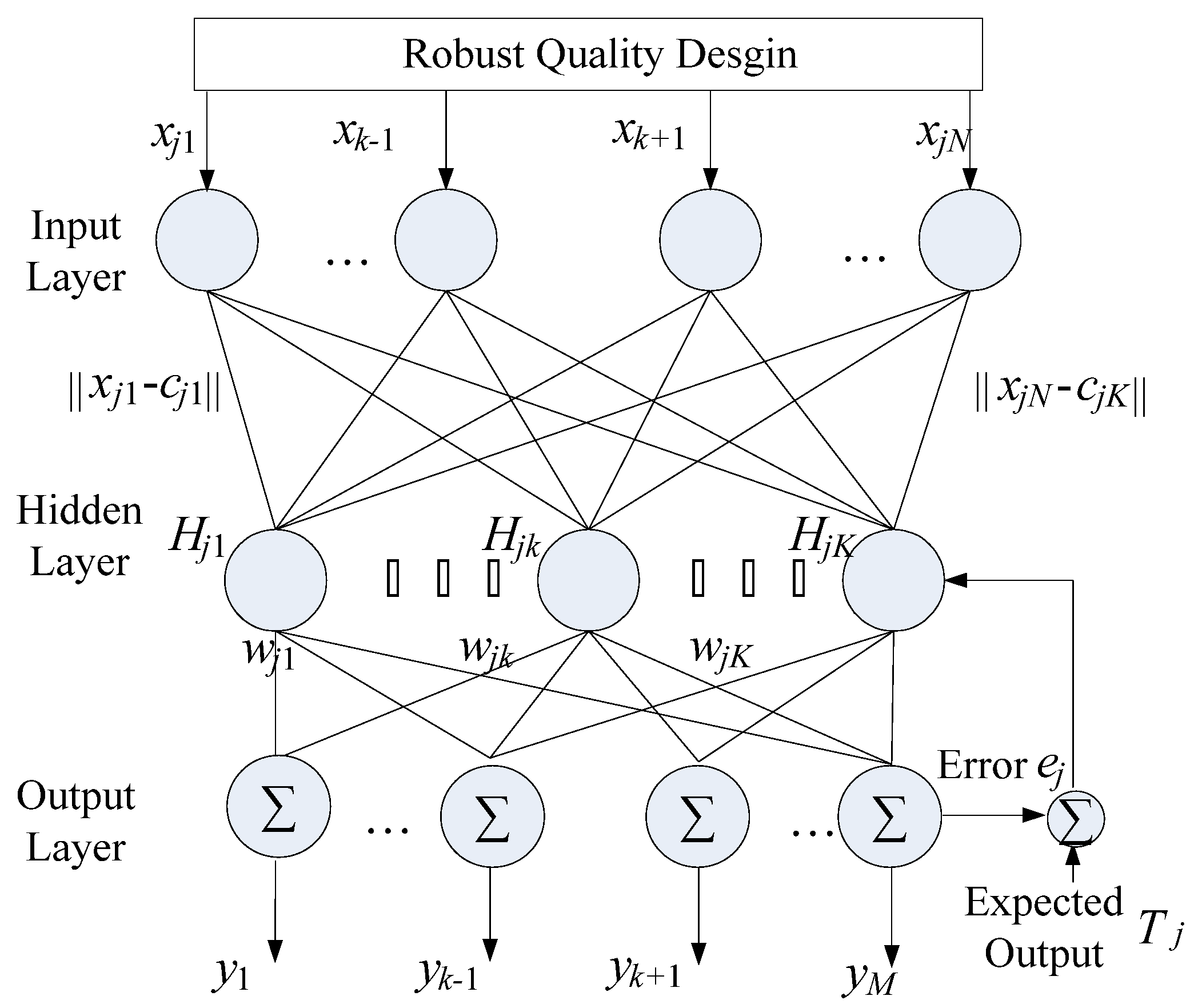
Enhanced Radial Basis Function Networks (ERBFNs) consist of the input, hidden, and output layers. The ERBFN structure is shown in Figure 1. The unknown j-th input vector $X_j=\left[x_{j1}, x_{j2},\cdots , x_{ji}, \cdots , x_{jN}\right]$, i = 1, 2, …, N, j = 1, 2, …, M, is connected to the input layer.

The number of output nodes yj, j = 1, 2, …, M, is equal to the number of training input–output data pairs, i.e., the input nodes (a matrix) and output nodes (a vector) are paired. The j-th hidden nodes vector $H_j=\left[H_{j1}, H_{j2},\cdots , H_{ji}, \cdots , H_{jK}\right]$, k = 1, 2, …, K, j = 1, 2, …, M. The weights w_jk connect the k-th hidden node with the j-th output node.

3.1. Input Layer

In this paper, xi is the i-th variable of the expected output. For each training data pair, set the input matrix as X = [xji] M × N, j = 1, 2, …, M, i = 1, 2, …, N.

3.2. Hidden Layer

In the hidden layer, $C_j=[ c_{j1}, \dots . , c_{jk} , \dots . , c_{jK}]$ is called the j-th center of the ERBFN. $\left|\right|x_{ji}-c_{jk}\left|\right|$ is the Euclidean distance between the i-th node of the input layer and the k-th node of the hidden layer. The Euclidean distance is determined by Equation (2). The k-th hidden layer output is defined as Equation (3):

$$\Vert x_{ji}-c_{jk}\Vert =\sqrt{{\displaystyle \sum _{i=1}^N{(x_{ji}^{}-c_{jk})}^2}}$$

(2)

$$H_{jk}^{}={\phi }_{jk}^{}(\sqrt{{\displaystyle \sum _{i=1}^N{(x_{ji}^{}-c_{jk})}^2}})$$

(3)

$$\phi (x)=e^{-x^2/{\sigma }^2}$$

(4)

where, in Equation (4), the function $\phi \left(·\right)$ is a Gaussian distribution function, and σ is a smoothing parameter.

3.3. Output Layer

In the output layer, let w_jk be the weight between hidden node H_jk and output node y_j and the j-th output of the output layer be as in Equation (5).

$$y_j={\displaystyle \sum _{k=1}^{K}w{}_{jk}{}^{}H{}_{jk}^{} , j=1,2,\dots ,M}$$

(5)

The error between the simulation output y_j and its expected value T_j is calculated by an error function. The error function is defined as Equation (6):

$$\begin{array}{l}{e}_j^{}(n)={\left[T_j-y_j(n)\right]}^{{ }^2}\\ ={\left[T_j-{\displaystyle \sum _{k=1}^K{w}_{jk}(n)\exp \left(-\frac{{\Vert X_j(n)-C_{jk}(n)\Vert }^2}{{\sigma }_{jk}^2(n)}\right)}\right]}^2\end{array}$$

(6)

where e_j(n) and y_j(n) are the j-th error and the j-th simulation output of the n-th epoch, respectively.

In order to adjust three parameters, which are weights w_jk, the center of ERBFN C and the smoothing parameters σ_jk of function $\phi \left(·\right)$, the related parameters are updated by Equations (7)–(9).

$$w_{jk}(n+1)=w_{jk(n)}-{\mu }_{jw}\frac{\partial }{\partial w_{jk}}{e}_j(n)$$

(7)

$$c_{jk}(n+1)=c_{jk(n)}-{\mu }_{jc}\frac{\partial }{\partial c_{jk}}{e}_j(n)$$

(8)

$${\sigma }_{jk}(n+1)={\sigma }_{jk(n)}-{\mu }_{j\sigma }\frac{\partial }{\partial {\sigma }_{jk}}{e}_j(n)$$

(9)

3.4. Stopping Criteria

One thousand generations (Epoch) or $e_j(n)\le 0.00001$ is set in this paper as the stopping criteria.

A trained enhanced radial basis function network was used for fault diagnosis, as shown in Figure 2. The parameters to be tested $x_1^{new},x_2^{new},\dots ,x_k^{new},\dots ,x_N^{new}$ for fault diagnosis were first input into the trained and convergent ERBFN, and then a set of outputs $x_1^{\prime },x_2^{\prime },\dots ,x_k^{\prime },\dots ,x_N^{\prime }$ could be outputted from the EBRFN. Equation (10) is used to obtain variations of the two parameter sets.

$${\Sigma }_i={\left(x_i^{new }-x_i^{\prime }\right)}^2 , i=1,2,\cdots N$$

(10)

For finding the fault sources, the parameters to be tested were observed at all their variations. As shown in Equation (11), $\epsilon$ is a very small number. In Equation (11), if each variation is very small and their values are very close to each other, this means that there is no fault source for the parameters to be tested, and the system is normal. Equation (12) means that the system is in a fault state, in which the variation is very small, and the other (N-1) ${\sigma }_{i}s$ are large. Simultaneously, the state indicates that $x_i$ is the fault sources, and this parameter sensor fails.

$$({\sigma }_1\cong {\sigma }_2\cong \dots .\cong {\sigma }_N)<\epsilon ({\mathsf{\sigma }}_1\approx {\mathsf{\sigma }}_2\approx \cdots \approx {\mathsf{\sigma }}_{\mathrm{N}})<\mathsf{\epsilon }$$

(11)

$${\sigma }_k<\epsilon <{\sigma }_i i=1,2,\cdots , N i\ne k$$

(12)

Data of the ice-storage air-conditioning system were collected in this paper, including high pressure, low pressure, low-pressure return pipe temperature, brine outlet temperature, brine inlet temperature, brine flow rate, cooling water flow, and external air temperature. In the real world, training data can be collected from field data. ERBFN training is carried out in order to minimize the fitting error for a sample training set. For a given training data, the fitness function is defined as in Equation (6). The new training data are presented to the ERBFN, and the corresponding hidden nodes will continue to grow. Additionally, Equations (7)–(9) are used to adjust the relative parameters in order to minimize the fitting error for a sample training set. This process results in very fast training, and the network is adaptive to data changes. The diagnostic system’s database can always be enhanced, with each new sample added to the current database. Training data in the database can be selected for diagnosis, addition, and deletion with Matlab-Excel Link to construct the ERBFN. Matlab-Excel Link is a software add-on to integrate the Matlab computing environment and Excel workspace. It also provides data management with data from the Excel workspace and the evaluation command from the Matlab workspace. Excel workspace becomes a data-storage and application-development front end for Matlab, which is a computational processor for developing the diagnostic tool.

4. Test Results and Discussion

The proposed algorithm was tested in a hospital with six chillers (two sets of 550RT chillers and four sets of 1000RT chillers and an 18,000RT-h ice storage tank. Data of the ice-storage-air-conditioning system were measured in the field. Simulations were carried out with MATLAB 7.6 on a Core i5-7300HQ, 2.5 GHz personal computer with 8 GB of RAM. The Excel file was used to store 1746 training data with Matlab-Excel Link to construct a computational process. We have 1744 training data for the ERBFN with four operational types and eight key data. To show the effectiveness of the proposed diagnostic system, three cases were chosen for investigation.

4.1. Robust Parameter Design

Seven factors with three levels and one factor with two levels that were consistent with the orthogonal table of Table 3 were selected from the historical data of brine chillers’ operation. The effect analysis in the orthogonal table shows the optimal experimental parameter combinations of the effects, namely A–H in Table 2. This parameter set represents the optimal effects of this period selected from the historical data. Therefore, provided that the control logic of the brine chiller is correct, without violating natural physical constraints, this parameter set must be an undisturbed measured value. If the controller controls the brine chiller with disturbed parameters, the brine chiller must run in poor operating conditions. For example, the distortion of low pressure will make the refrigerant superheat of the brine chiller too high or too low. Too high superheat makes the electronic expansion valve open too large so that too many refrigerants will enter the suction end of the refrigerant circulation system, and some liquid refrigerants will run into the compressor, resulting in an instant increase in the compressor’s energy consumption, efficiency decrease, and damage to the compressor. On the other hand, too low superheat makes the electronic expansion valve open too small so that too few refrigerants will enter the evaporator and the pressure is too low, leading to an increase in the compressor’s energy consumption, efficiency decrease, and even triggering the low-pressure alarm (false alarm).

Table 5. Control factors and their levels.

Factor	Explanation	Level 1	Level 2	Level 3
A	external air temperature (°C)	24.2	24.1
B	high pressure (kgf/cm2)	7.4	7.5	7.6
C	low pressure (kgf/cm2)	1.1	1.2	1.3
D	low-pressure return pipe temperature (°C)	−9.1	−8.9	−8.8
E	brine outlet temperature (°C)	−4.5	−4.4	−4.1
F	brine inlet temperature (°C)	−2.3	−2.2	−2.1
G	cooling outlet water temperature (°C)	29.9	30.1	30.2
H	cooling inlet water temperature (°C)	27.2	27.3	27.4

shows the analysis parameters of the orthogonal table to be used in this experiment.

Except for the experiment with optimal effects, other experiments indicate that the parameters used may be interfered with by other factors. The optimal effect parameters from the analysis of an orthogonal table were considered as the signals measured by the health sensor in this study because disturbed parameters cannot make the brine chiller have good effects when the control logic of the brine chiller is correct, and the optimal effect (electricity consumption per ton) is the control objective. Even if the parameter set with the optimal effect does not fully conform to the physical identical equation, the fault diagnosis ability of the enhanced radial basis function network will not be affected, which is one of the biggest advantages of artificial neural networks. In contrast, these experiments with different levels of parameters could be considered to be caused by interference or drift. The parameters selected by robust quality design were input into the radial basis function network for training until the artificial neural network converged. After training data were pre-processed by robust quality design, the trained artificial neural network could be used to judge whether the brine chiller was in a normal state, as shown in

Table 6. L₁₈ (2¹ × 3⁷) orthogonal array (KW/USRT).

Exp	A	B	C	D	E	F	G	H	M1 (%)		M2 (%)		Ave. (KW/USRT)	S/N
									N1	N2	N1	N2
1	1	1	1	1	1	1	1	1	0.847	0.845	0.815	0.842	0.837	1.542
2	1	1	2	2	2	2	2	2	0.849	0.832	0.812	0.835	0.832	1.596
3	1	1	3	3	3	3	3	3	0.851	0.837	0.828	0.791	0.827	1.649
4	1	2	1	1	2	2	3	3	0.797	0.849	0.819	0.850	0.829	1.628
5	1	2	2	2	3	3	1	1	0.845	0.834	0.837	0.844	0.840	1.514
6	1	2	3	3	1	1	2	2	0.868	0.841	0.815	0.849	0.843	1.479
7	1	3	1	2	1	3	2	3	0.823	0.833	0.790	0.831	0.819	1.730
8	1	3	2	3	2	1	3	1	0.796	0.847	0.829	0.824	0.824	1.679
9	1	3	3	1	3	2	1	2	0.809	0.834	0.792	0.836	0.818	1.745
10	2	1	1	3	3	2	2	1	0.831	0.851	0.836	0.858	0.844	1.472
11	2	1	2	1	1	3	3	1	0.823	0.832	0.842	0.801	0.825	1.675
12	2	1	3	2	2	1	1	3	0.850	0.807	0.850	0.851	0.840	1.517
13	2	2	1	2	3	1	3	2	0.844	0.838	0.798	0.852	0.833	1.584
14	2	2	2	3	1	2	1	3	0.799	0.837	0.808	0.795	0.810	1.831
15	2	2	3	1	2	3	2	1	0.808	0.822	0.819	0.833	0.821	1.718
16	2	3	1	3	2	3	1	2	0.845	0.849	0.851	0.825	0.843	1.488
17	2	3	2	1	3	1	2	3	0.797	0.811	0.848	0.817	0.818	1.740
18	2	3	3	2	1	2	3	1	0.862	0.843	0.793	0.809	0.827	1.648

.

Table 6 and

Table 7. Effect Response Table.

	A	B	C	D	E	F	G	H
Level 1 (S/N)	1.618	1.575	1.574	1.675	1.651	1.590	1.606	1.596
Level 2 (S/N)	1.630	1.626	1.673	1.598	1.605	1.654	1.623	1.595
Level 3 (S/N)	□	1.672	1.626	1.600	1.618	1.629	1.644	1.683
Effect	0.012	0.096	0.099	0.076	0.046	0.063	0.038	0.088
Rank	8	2	1	4	6	5	7	3

show the robust quality design experiment results and its factor response, respectively. The data in Table 7 are calculated based on robust quality design principles. There are 8 factors in Table 7, and these factors affect the performance of a chiller. From Table 7, we can obtain the effect of each factor on the experimental system. According to Table 7 and Figure 3, the optimal combinations of the robust quality design are as follows:

Table 8. Best Factor Combination.

Best Factor	Factor	Value
A2	external air temperature (°C)	24.1
B3	high pressure (kgf/cm2)	7.6
C2	low pressure (kgf/cm2)	1.2
D1	low-pressure return pipe temperature (°C)	−9.1
E1	brine outlet temperature (°C)	−4.5
F2	brine inlet temperature (°C)	−2.2
G3	cooling outlet water temperature (°C)	30.2
H3	cooling inlet water temperature (°C)	27.4

shows the values of optimal factors. The parameters selected by Taguchi’s orthogonal experiment were used as the training data to be input into the radial basis function network, and the artificial neural network trained with a large number of parameters obtained through the robust quality design would be complete. As these parameters selected by the robust orthogonal design can make the brine chiller in the ice-storage-air-conditioning system run at high efficiency, it can be identified that the system runs in a normal state. No matter whether the input data are the actual historical data or violate the real physical constraints of the system, artificial neural networks trained with a large number of data can provide low-error predicted values for the to-be-detected inputs in the future.

4.2. The Efficacy Analysis of RBFN

Figure 4 shows the prediction of a brine chiller’s efficacy by using RBFN. From Figure 4, most of the predicted values are close to the true value; that is, RBFN has the ability to predict and identify the operation status of a brine chiller. However, it can also be shown from Figure 4 (High Pressure, HP) that some predicted values are not very accurate, and the largest prediction is as high as 5% or more. Obviously, if only the RBFN is used to perform the fault diagnosis of the brine chiller, it is very likely to generate false alarms. The reason for the false alarm is probably that the RBFN is distributed by various uncertain factors. Therefore, robust parameter design is applied to data preprocessing tools for RBFN. Since undistributed healthy signals are selected through robust parameter design, the diagnostic capability of RBFN will be enhanced.

In addition, the sensitivity of RBFN fault diagnosis mainly depends on the quantity and quality of training samples (Figure 5).

4.3. Fault Diagnosis of ERBFN

Historical data were used as the samples to train ERBFN, and the converged ERBFN after training were used to determine whether there were anomalies in the brine chiller and find fault sources. As shown in

Table 9. The results of fault diagnosis.

Case	σA	σB	σC	σD	σE	σF	σG	σH	State
1	0.0015	0.0024	0.0024	0.0011	0.0017	0.0020	0.0018	0.0013	Normal
2	0.0068	0.0099	0.0122	0.0172	0.0204	0.0195	0.0179	0.0192	OA offset
3	0.0042	0.0028	0.0078	0.0041	0.0051	0.0076	0.0054	0.0078	HP offset
4	0.0118	0.0082	0.0012	0.0046	0.0098	0.0089	0.0101	0.0079	LP offset
5	0.0116	0.0104	0.0099	0.0063	0.0121	0.0091	0.0078	0.0083	LR offset

OA offset: Outside Air Temperature Offset. HP offset: High-Pressure Offset. LP offset: Low-Pressure Offset. LR offset: low-pressure return pipe temperature.

, there are parameters of eight orthogonal tables in this experiment, indicating eight sensor failure sources of the brine chiller. The fault diagnosis results are shown in Table 9; if there was no fault in the brine system (Case 1), the diagnostic variations of eight sensors (σA, σB, σC, σD, σE, σF, σG, σH) were very small. According to Equation (11), Case 1 can be used to determine that the brine chiller is in a normal state. According to Equation (12), the diagnostic variation σA of parameter A (external air temperature) is very small, and the variations of other parameters are significantly large. In Case 2, its fault source is an external air temperature sensor. By the same analysis, the fault sources of Cases 3 to 5 are, respectively, parameter B of the high-pressure sensor, parameter C of the low-pressure sensor, and D of the low-pressure return pipe temperature sensor.

In this research, a fault simulator was used, as shown in Equation (13), to simulate the signal drift of the sensor.

$$x_i={\overline{x}}_i+f_i+v_i , i=1,2,\dots .,N$$

(13)

where ${\overline{x}}_i$ is the true value; $f_i$ is the drift value; and $v_i$ is the interference. In this study, the drift value was set at 10% and the interference was set at 5%. In fact, signal drift is common in systems. However, as some special situations are different from the training samples of artificial neural networks, ERBFN may make incorrect diagnoses; hence, the system can still generate fault alarms in a normal state. In order to avoid fault alarms, more system operating states need to be trained. In addition to fault alarms, missed alarms often occur in real systems. Artificial neural networks may not be able to detect minor faults because the data of minor faults are similar to those of the normal state. Fault sample accumulation should be able to avoid missed alarms and increase the success rate of fault diagnosis.

5. Conclusions

This paper proposes a fault diagnosing system for the ice-storage air-conditioning system, which is used to supervise the operation status of a chiller and detect possible fault sources in advance. The important contributions of this paper are as follows: (1.) This paper provides a system fault diagnosis method based on the artificial intelligence algorithm, ERBFN. (2.) This paper successfully integrates artificial neural network and Robust Quality Design (RQD) into a new high-efficiency artificial intelligence algorithm ERBFN. (3.) This paper successfully uses RQD to select the best operating parameters of a chiller and uses these parameters to establish an artificial neural network training database. (4.) This paper successfully uses RDQ to improve the robustness and search ability of the AI algorithm. (5.) In this paper, ERBFN is successfully used to perform fault diagnosis of the ice-storage air-conditioning system. The new artificial neural network algorithm proposed in this research was successfully applied to the fault diagnosis and fault prediction of ice-storage air-conditioning systems. It not only provides a reference for enterprises but can also be applied to studies on other topics in the future. The proposed algorithm should be a considerable academic contribution. When enterprises have energy saving and warranty issues, the findings of this research can be provided as a strategic policy to which enterprises can adhere. Meanwhile, this improvement can also increase company competitiveness and sustainable management abilities while enriching the existing studies on air conditioning energy saving.

References

1. Stoecker, W.F.; Jones, J.W. Refrigeration and Air Conditioning, 2nd ed.; McGraw-Hill, Inc.: New York, NY, USA, 1982. [Google Scholar]
2. Mancin, S.; Noro, M. Reversible Heat Pump Coupled with Ground Ice Storage for Annual Air Conditioning: An Energy Analysis. Energies 2020, 13, 6182. [Google Scholar] [CrossRef]
3. Lin, W.M.; Tu, C.T.; Tsai, M.T.; Lo, C.C. Optimal Energy Reduction Schedules for Ice Storage Air-Conditioning Systems. Energies 2015, 8, 10504–10521. [Google Scholar] [CrossRef] [Green Version]
4. Rismanchi, B.; Saidur, R.; Masjuki, H.H.; Mahlia, T.M. Energetic, economic and environment benefits of utilizing the ice thermal storage systems for office building application. Energy Build. 2012, 50, 347–354. [Google Scholar] [CrossRef]
5. Wu, S.; Sun, J.Q. A top-down strategy with temporal and spatial partition for fault detection and diagnosis of building HVAC systems. Energy Build. 2011, 43, 2134–2139. [Google Scholar] [CrossRef]
6. Sanaye, S.; Shirazi, A. Thermo-economic optimization of an ice thermal energy storage system for air-conditioning applications. Energy Build. 2013, 60, 100–109. [Google Scholar] [CrossRef]
7. Hajiah, A.; Krarti, M. Optimal control of building storage systems using both ice storage and thermal mass—Part II: Parametic analysis. Energy Convers. Manag. 2012, 64, 509–515. [Google Scholar] [CrossRef]
8. Dong, X.J.; Shen, J.N.; He, G.X.; Ma, Z.F.; He, Y.J. A general radial basis function neural network assisted hybrid modeling method for photovoltaic cell operating temperature prediction. Energies 2021, 234, 121212. [Google Scholar] [CrossRef]
9. Ogunleye, O.; Singh, R.M.; Cecinato, F. Assessing the thermal efficiency of energy tunnels using numerical methods and Taguchi statistical approach. Appl. Therm. Eng. 2021, 185, 116377. [Google Scholar] [CrossRef]
10. Mosca, E. Optimal predictive and adaptive control. In Prentice Hall International Editions; Prentice-Hall Inc.: Hoboken, NJ, USA, 1995. [Google Scholar]
11. Kang, Z.; Wang, R.; Zhou, X.; Feng, G. Research Status of Ice-storage Air-conditioning System. Procedia Eng. 2017, 205, 1741–1747. [Google Scholar] [CrossRef]
12. Yao, W.; Li, D.; Gao, L. Fault detection and diagnosis using tree-based ensemble learning methods and multivariate control charts for centrifugal chillers. J. Build. Eng. 2022, 51, 104243. [Google Scholar] [CrossRef]
13. Li, G.; Hu, Y.; Liu, J.; Fang, X.; Kang, J. Review on Fault Detection and Diagnosis Feature Engineering in Building Heating, Ventilation, Air Conditioning and Refrigeration Systems. IEEE Access 2021, 9, 2153–2187. [Google Scholar] [CrossRef]
14. Guo, Y.; Chen, H. Fault diagnosis of VRF air-conditioning system based on improved Gaussian mixture model with PCA approach. Int. J. Refrig. 2020, 118, 1–11. [Google Scholar] [CrossRef]
15. Zhu, X.; Du, Z.; Chen, Z.; Jin, X.; Huang, X. Hybrid model based refrigerant charge fault estimation for the data center air conditioning system. Int. J. Refrig. 2019, 106, 392–406. [Google Scholar] [CrossRef]
16. Rohit, C.; Jon, W.; Xin, J. Automated fault detection of residential air-conditioning systems using thermostat drive cycles. Energy Build. 2021, 236, 110691. [Google Scholar]
17. Wang, Y.; Li, Z.; Chen, H.; Zhang, J.; Liu, Q.; Wu, J.; Shen, L. Research on diagnostic strategy for faults in VRF air conditioning system using hybrid data mining methods. Energy Build. 2021, 247, 111144. [Google Scholar] [CrossRef]
18. Zhu, X.; Du, Z.; Jin, X.; Chen, Z. Fault diagnosis based operation risk evaluation for air conditioning systems in data centers. Build. Environ. 2019, 163, 106319. [Google Scholar] [CrossRef]
19. Guo, Y.; Tan, Z.; Chen, H.; Li, G.; Wang, J.; Huang, R.; Liu, J.; Ahmad, T. Deep learning-based fault diagnosis of variable refrigerant flow air-conditioning system for building energy saving. Appl. Energy 2018, 225, 732–745. [Google Scholar] [CrossRef]
20. Wu, J.D.; Liao, S.Y. Fault diagnosis of an automotive air-conditioner blower using noise emission signal. Expert Syst. Appl. 2010, 37, 1438–1445. [Google Scholar] [CrossRef]
21. Wu, J.D.; Liao, S.Y. A self-adaptive data analysis for fault diagnosis of an automotive air-conditioner blower. Expert Syst. Appl. 2011, 38, 545–552. [Google Scholar] [CrossRef]
22. Song, Y.K.; Akashi, Y.; Yee, J.J. A development of easy-to-use for fault detection and diagnosis in building air-conditioning systems. Energy Build. 2008, 40, 71–82. [Google Scholar] [CrossRef]
23. Du, Z.; Jin, X. Detection and diagnosis for sensor fault in HVAC system. Energy Convers. Manag. 2007, 48, 693–702. [Google Scholar] [CrossRef]
24. Du, Z.; Jin, X. Detection and diagnosis for multiple faults in VAV systems. Energy Build. 2007, 39, 923–934. [Google Scholar] [CrossRef]
25. Ghate, V.N.; Dudul, S.V. Optimal MLP neural network classifier for fault detection of three phase induction motor. Expert Syst. Appl. 2010, 37, 3468–3481. [Google Scholar] [CrossRef]
26. Ham, F.M.; Kostanic, I. Principal of Neurocomputing for Science and Engineering; McGraw-Hill Companies, Inc.: New York, NJ, USA, 2001. [Google Scholar]
27. Lin, W.M.; Yan, C.D.; Lin, C.H.; Tsay, M.T. A Fault Classification Method by RBF Neural Network with OLS Learning Procedure. IEEE Trans. Power Deliv. 2001, 16, 473–477. [Google Scholar] [CrossRef]
28. Ross, P.J. Taguchi Techniques for Quality Engineering, 2nd ed.; McGraw-Hill Companies, Inc.: New York, NY, USA, 1988; pp. 203–243. [Google Scholar]
Figure 1. The ERBFN structure.
Energies 15 03981 g001
Figure 2. Diagram of ERBFN fault diagnosis.
Energies 15 03981 g002
Figure 3. The Construction of Factor Response.
Energies 15 03981 g003
Figure 4. The prediction of a brine chiller’s efficacy.
Energies 15 03981 g004
Figure 5. The variance curve of brine inlet water temperature T1 diagnosis efficiency test.
Energies 15 03981 g005