Heuristic Intrusion Detection Based on Traffic Flow Statistical Analysis

Abstract

As telecommunications are becoming increasingly important for modern systems, ensuring secure data transmission is getting more and more critical. Specialised numerous devices that form smart grids are a potential attack vector and therefore is a challenge for cybersecurity. It requires the continuous development of methods to counteract this risk. This paper presents a heuristic approach to detecting threats in network traffic using statistical analysis of packet flows. The important advantage of this method is ability of intrusion detection also in encrypted transmissions. Flow information is processing by neural networks to detect malicious traffic. The architectures of subsequent versions of the artificial neural networks were generated based on the results obtained by previous iterations by searching the hyperparameter space, resulting in more refined models. Finally, the networks prepared in this way exhibited high performance while maintaining a small size—thereby making them an effective method of attacks detection in network environment to protect smart grids.

1. Introduction

Cybersecurity is a challenge of smart grids [1,2,3]. The rise of digitization brings many benefits but also creates potential risks. The number of attack vectors and the amount of available data are constantly growing [4,5]. To ensure the security of rapidly evolving networks, new methods of attack detection must be developed.

The remainder of the paper proceeds as follows: Section 2 provides an introduction to cybersecurity, neural networks, and detection methods. Dataset and its modifications are shown in Section 3. The creation of heuristic algorithms is presented in Section 4. The experimental results are presented and discussed in Section 5. Finally, Section 6 contains discussion of results and Section 7 concludes the paper.

1.1. Rationale

Network attack detection is a costly process. Current methods mostly rely on signatures, the presence of characteristic features of attacks. An example of software that uses this methodology is Snort. Such an approach is very effective but has significant limitations.

The first disadvantage is the inability to detect new attacks (so-called zero-day). Often, a small change in the signature by replacing one or more bits in a packet avoids detection while maintaining the underlying threat. Stopping such a modified attack requires manual alteration of the signature.

Another disadvantage is the limited ability to work with encrypted traffic. Some signatures are based on information that is usually encrypted. Since encryption is omnipresent, these signatures cannot be used without costly decryption of the communication. Additionally, effective detection on higher layers requires storing packets that are fragments of the complete message being transmitted. This approach becomes unachievable in networks that generate a lot of traffic.

Machine learning, especially using artificial neural networks, is able to overcome these problems. With their ability to generalise, making small changes to attacks will not allow detection to be bypassed. The characteristics of attacks are learned automatically by finding anomalies. It reduces the need for manual modification. Additionally, an approach based on flow statistics performs detection of encrypted traffic without decryption and packet storage.

1.2. Related Works

Two main types of intrusion detection approaches can be distinguished: algorithms based on the predefined attacks’ signatures [6] and methods analysing behaviours to detect anomalies in network traffic [7]. The second group contains machine learning to detect threats—a common research topic now [8,9,10].

Dini et al. [11] used K-nearest neighbors and artificial neural network. Both methods achieved high performance on datasets created from simulating a US Air Force LAN. However, the dataset was relatively small. Kao et al. [12] used a two-stage method. It utilised Denoising Auto-Encoder (DAE) and Gate Recurrent Units (GRU). Achieved accuracy was over 90%. Ullah et al. [13] proposed a hybrid neural network containing long short-term memory (LSTM) and gated recurrent unit (GRU). Multiple datasets were merged into DDoS and car hacks sets. The corresponding accuracy were 99.5% and 99.9%. The combined datasets did not contain all of the original data, which may have affected the results. Almaraz-Rivera et al. [14] tested multiple models, including Support Vector Machine (SVM), Decision Tree and Long-Short Term Memory (LSTM). Part of the Bot-IoT dataset used was imbalanced and most samples were attack attempts. Few methods obtained nearly 100% accuracy. Le et al. [15] used convolutional neural network (CNN). Additionally, a generative adversarial network (GAN) was used to produce extra samples. The results reached approximately 0.97 F-score. Kurt et al. [16] defined attack as a partially observable Markov decision process (POMDP) problem. The proposed reinforcement learning (RL) algorithm has the ability to detect anomalies in smart grid networks in real-time. Boyaci et al. [17] proposed an algorithm based on graph neural network (GNN) to detect and localise false data injection (FDIA) attacks. He et al. [18] proposed a conditional deep belief network (CDBN) and tested it on IEEE 118-bus and IEEE 300-bus systems.

1.3. Contributions

The main contributions of this work are summarised as follows:

• The authors have chosen heuristic detection approach based on traffic flow statistical analysis. It supports attack detection in encrypted network traffic.
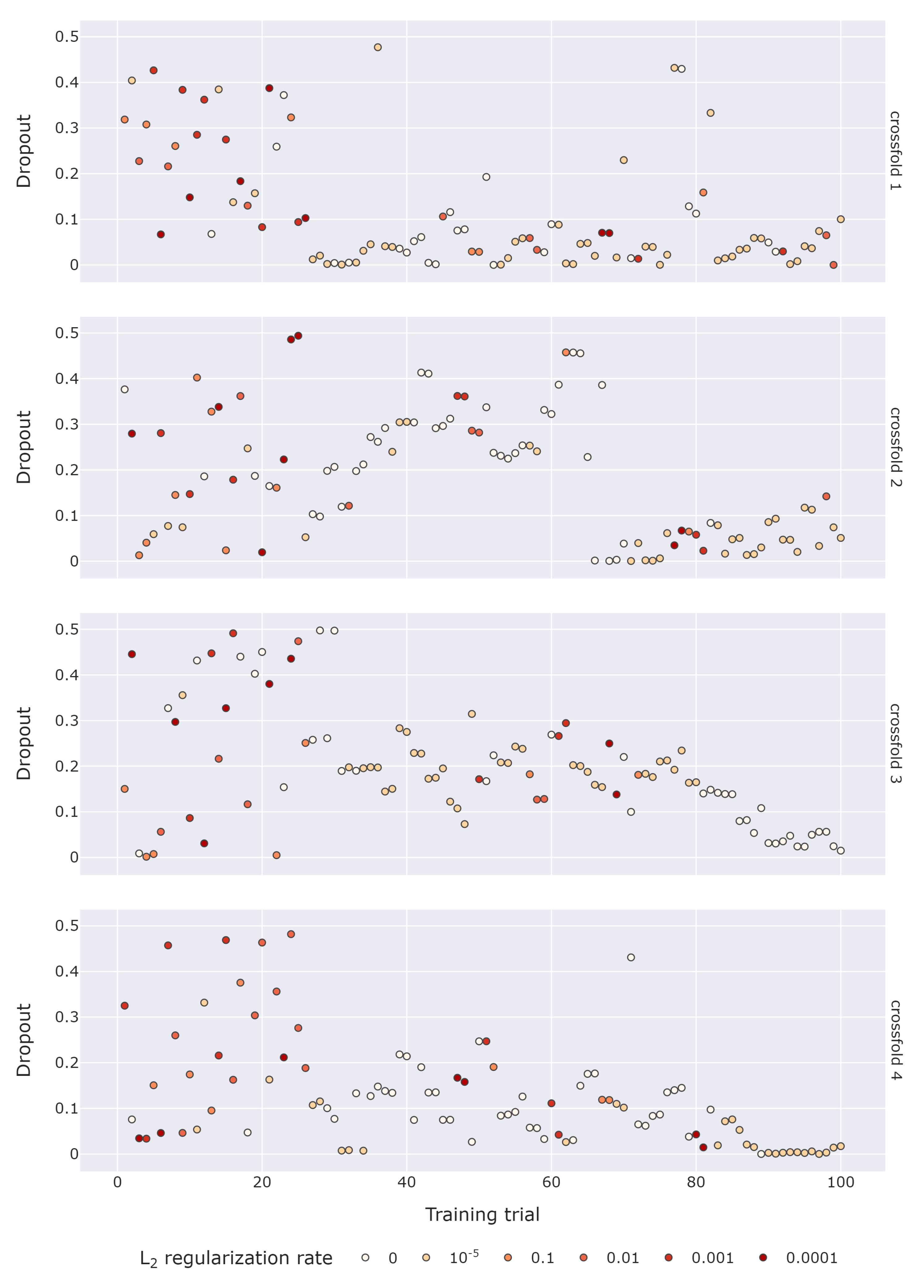
• The process of searching the hyperparameter space to create neural network with high performance in detecting network attacks was presented. The assessment is focused on the ${\mathrm{F}}_2$ score metric, which prioritises marking packets as representing an attack over reducing false alarms.
• A modified normalization method was used. This solution provides better performance during the conducted trials.

2. Cybersecurity and Artificial Intelligence

Cybersecurity is a very broad concept. In short, it is the assurance of security for computer systems and networks [19]. The importance of electronic devices is growing more and more these days. This is ubiquitous and essential for automation and communication in the modern world. The increase in its presence also raises the likelihood and magnitude of threats arising from it.

Network security is provided by the devices of which a network consists. Firewalls are specialised equipment designed to prevent attacks through analysis of traffic. Usually, they operate as part of an Intrusion Prevention System (IPS)—they detect threats and block them. Intrusion Detection System (IDS) only detects the occurrence of an attack, without taking further action. However, it is not always possible to discover a malicious activity at the very beginning of an attack.

Threat detection might rely on signatures or anomalies [20,21]. In this paper, neural networks are used for anomaly detection and they are considered a heuristic approach [22]. There is no absolute confidence in the correctness of the prediction, but the results can be good enough for practical purposes. They might outperform the speed of the signature based approach.

2.1. Artificial Neural Networks

Machine learning is a subset of artificial intelligence. These are algorithms that are capable of learning autonomously from available data to accomplish their goal [23]. There are a plethora of different approaches and architectures. In machine learning, numerous types of models are distinguished including decision trees, support vector machine, Bayesian methods, neural networks and others.

Nowadays, the most rapidly growing domain of machine learning is neural networks, particularly deep learning, which is a subset of them. This field has wide applications for which various architectures are used depending on the data available and the expected outcome. A multilayer perceptron (MLP) [24] network was employed to perform network attack detection from statistical information about the flow in this paper.

An MLP can consist of a varying number of layers. Each layer can contain a different number of nodes called neurons. These layers are known as dense because each value returned by the neurons of a layer is used by each neuron of the next layer.

A neuron defined that way is restricted to linear regression due to the absence of nonlinearities. This limitation is solved by using an activation function to introduce nonlinearities. Examples of such functions are ReLU, LeakyReLU [25], and Swish [26] expressed successively by the equations:

$$\varphi \left(z\right)=max(0,z)$$

(1)

$$\varphi \left(z\right)=max(\alpha z,z)$$

(2)

$$\varphi \left(z\right)=\frac{z}{1+e^{-z}}$$

(3)

where z is output of neuron, and $\alpha$ is a variable within the interval $(0,1)$.

The learning of neural networks is done by a backpropagation algorithm. One of its modification is called Adam [27] (adaptive moment estimation), which is one the most popular optimization algorithms. This method combines RMSProp [28] and AdaGrad [29] allowing for even faster adjustment of weights.

By optimizing the loss function, the network adapts to the training set. One of the advantages of neural networks is the ability to generalise, a capability that could be forfeited by overfitting. For the classification problem, it involves accurately remembering the values of features belonging to categories, which allows us to classify elements of the training set with high confidence; however, this does not translate to the validation set, having virtually no identical samples. While increasing the size increases the potential capabilities of the model, the susceptibility to overfitting also becomes greater. Therefore, some techniques have been developed to mitigate this phenomenon.

The first technique is regularization [30]. It involves adding a value to the loss function that depends on the network coefficients to serve as a penalty to reduce their magnitude. The purpose of this action is to counteract overfitting. The following formula is often applied:

$${\mathrm{L}}_x=\sum _i{\left|\alpha {\theta }_i\right|}^x$$

(4)

where i is the index of the coefficient, and $\alpha$ is the penalty factor. The value of x is most often replaced by 1 to obtain the ${\mathrm{L}}_1$ loss or 2 to form the ${\mathrm{L}}_2$ loss. It is also possible to combine these two functions using their sum. Although $\alpha$ and x can be different for each coefficient, in most cases, they are identical for the entire network or layer. Regularization can be applied to biases b, although it is not recommended. Most often, it only limits the weights w.

Another technique to prevent overfitting is dropout [31]. It involves randomly setting some of the inputs to the neurons as 0 with probability d for each. The remaining values are scaled according to the formula:

$$x^{\prime }=\frac{x}{1-d}$$

(5)

so that the sum remains unchanged. The action is justified by preventing reliance on only selected features and assigning large weights to them, but promotes discovery of relationships between all features which alleviates the problem of missing a particular input. Dropout is only applied when training the network and may cause the performance on the validation set outperforms that on the training set where dropout was applied.

2.2. Performance Indexes

Appropriate measurement methodologies must be selected when designing an experiment. The classification approach involves finding the category to which a given sample belongs. For the binary classification adopted in this paper, only two conditions are present—Positive (P) and Negative (N). The assignment to classes only swaps the numerical values of the analogous derivative metrics. Considering the greater focus on detecting attacks rather than the absence of them, P condition was assigned to malicious traffic, while N condition was given to a benign one.

Binary classification algorithms make a decision based on whether the threshold is exceeded. If the value obtained lies above the threshold, the sample is classified as positive. While obtaining a lower value classifies the sample as negative, if the algorithm correctly classifies the sample, then the prediction for class P is referred to as True Positive (TP) and for class N as True Negative (TN).

A classification of the sample N as P results in a False Positive (FP) prediction. This is a Type I error resulting in a false alarm. In the case of IDS, this is classifying benign traffic as an attack attempt. Classification of sample P as N results in a False Negative (FN) prediction. This is a Type II error showing a miss. For an attempted attack, it is a failure to detect one.

The basic metric used in classification is accuracy (ACC). It is expressed by the formula:

$$\mathrm{accuracy}=\frac{\mathrm{TP}+\mathrm{TN}}{\mathrm{P}+\mathrm{N}}=\frac{\mathrm{TP}+\mathrm{TN}}{\mathrm{TP}+\mathrm{TN}+\mathrm{FP}+\mathrm{FN}}$$

(6)

Accuracy compares the ratio of correctly assigned labels to all checked samples. Its disadvantage is the necessity of balanced sample quantities among classes. In the case of a heavily unbalanced dataset, predicting only the most frequently occurring category yields a decent result, but this does not indicate that the algorithm is performing well, as it neglects the less frequent samples. For this reason, in the case of an unbalanced set, different metrics are applied in addition or instead.

Recall also referred to as sensitivity, recall, hit rate, or true positive rate (TPR) is one metric better indicating the effectiveness of classification on unbalanced datasets. Expressed by the formula:

$$\mathrm{recall}=\frac{\mathrm{TP}}{\mathrm{P}}=\frac{\mathrm{TP}}{\mathrm{TP}+\mathrm{FN}}$$

(7)

recall is the quotient of correctly classified positive samples (TP) to all positive samples. Actual negative labels are not taken into consideration. This is important when the P class is significantly underrepresented. The problem that arises from using this metric alone is the promoting of marking all samples as positive to maximise its value. For this reason, recall is not used as the sole metric, but rather as only one of many to analyse the problem.

Precision also referred to as positive predictive value (PPV) is another metric for evaluating the performance of algorithms on unbalanced datasets. The formula is:

$$\mathrm{precision}=\frac{\mathrm{TP}}{\mathrm{TP}+\mathrm{FP}}$$

(8)

In contrast to recall, the denominator is the number of samples classified as positive, rather than the real number. Precision introduces, in a way, a penalty for incorrectly labeling negative samples as positive. Again, it cannot be relied upon as an exclusive metric, as it promotes restrained assignment to the positive class.

An ${\mathrm{F}}_1$ score is next metric. It is the harmonic mean of recall and precision given by the formula:

$${\mathrm{F}}_1=\frac{2}{{\mathrm{recall}}^{-1}+{\mathrm{precision}}^{-1}}=2\times \frac{\mathrm{precision}\times \mathrm{recall}}{\mathrm{precision}+\mathrm{recall}}$$

(9)

${\mathrm{F}}_1$ score incorporates both of its components. The resulting values are in the range from 0 to 1. Obtaining greater values requires high recall as well as precision. A generalised version is the ${\mathrm{F}}_{\beta }$ score expressed by the formula:

$${\mathrm{F}}_{\beta }=(1+{\beta }^2)\times \frac{\mathrm{precision}\times \mathrm{recall}}{({\beta }^2\times \mathrm{precision})+\mathrm{recall}}$$

(10)

The $\beta$ coefficient is responsible for the weight of the factors. Values below 1 and greater than 0 assign higher weight to precision. Conversely, values greater than 1 give higher weight to recall. Depending on the $\beta$ value selected, the name of the metric is changed. In this paper, the authors decided to put more emphasis on recall; therefore, $\beta$ was set to 2, and the metric ${\mathrm{F}}_2$ score was applied.

3. Dataset

The dataset is an essential element during the development of a network threat detection algorithm. Although it is possible to create an anomaly detection algorithm based on a dataset containing only benign traffic, having malicious samples enables learning its characteristics and verifying performance.

3.1. Dataset Description

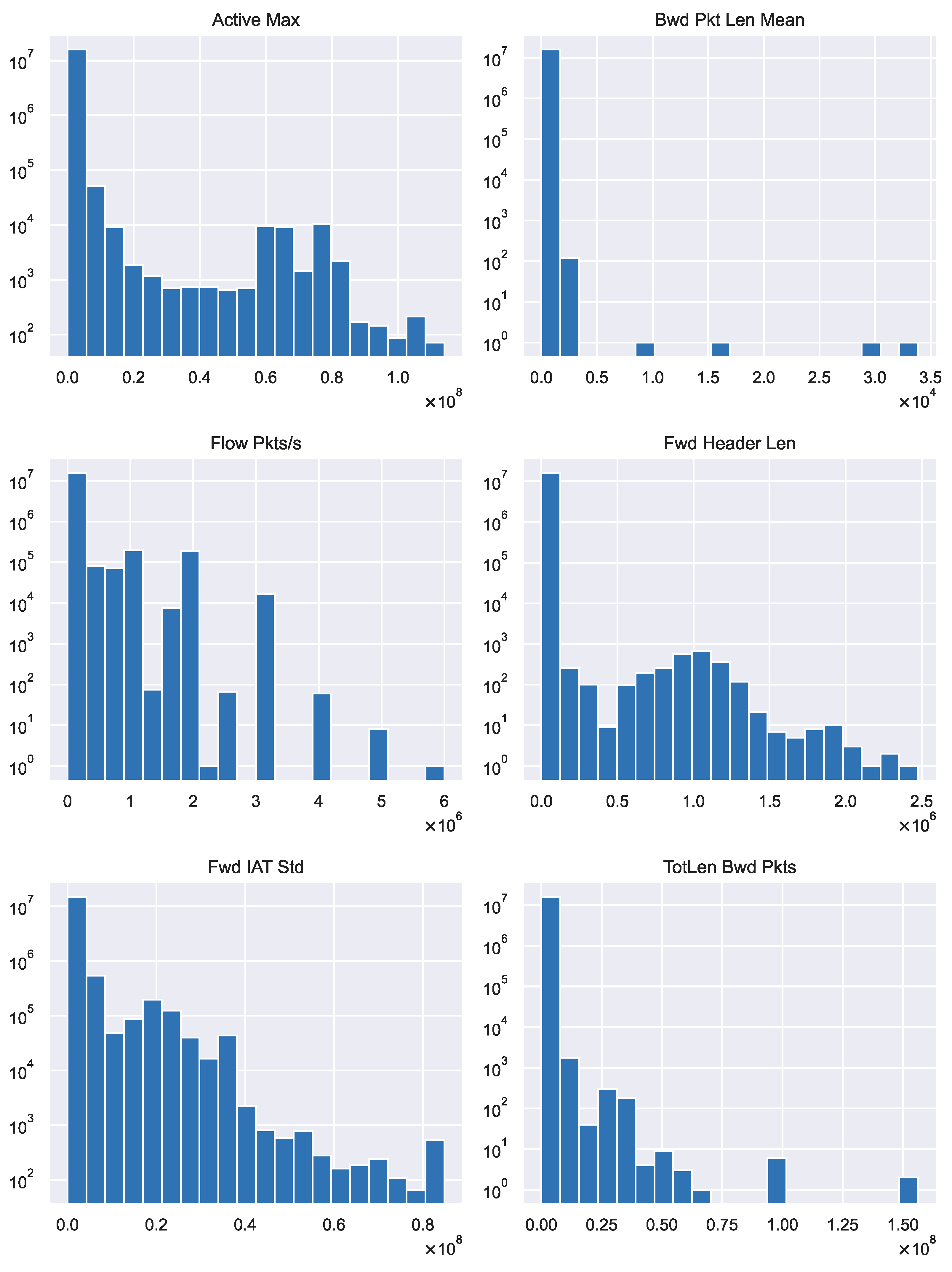
The CSE-CIC-IDS2018 [32] dataset was chosen to train the models. It was created using a network consisting of a total of 500 appliances. HTTPS, HTTP, SMTP, POP3, IMAP, SSH, and FTP protocols were used in the simulations. According to the observations, the majority of the traffic was HTTP and HTTPS. The environment contained both Linux and Windows operating system devices.

The CSE-CIC-IDS2018 provides both all packets constituting traffic in the prepared network as well as statistical information about the flows. Due to the enormous overhead required for processing individual packets, the resources for which might not be sufficient in a real network devices, a flow-based approach was adopted.

This dataset contains traffic related to following attacks: Brute-force attack, Heartbleed attack, Botnet, Denial-of-Service, Distributed Denial-of-Service, Web Attacks, and Infiltration of the network from inside. The counts of traffic categories are displayed in

Table 1. Types of flows in dataset with number of occurrences.

Type	Count
Benign	13,390,234
DDOS attack-HOIC	686,012
DDoS attacks-LOIC-HTTP	576,191
DoS attacks-Hulk	461,912
Bot	286,191
FTP-BruteForce	193,354
SSH-Bruteforce	187,589
Infiltration	160,639
DoS attacks-SlowHTTPTest	139,890
DoS attacks-GoldenEye	41,508
DoS attacks-Slowloris	10,990
DDOS attack-LOIC-UDP	1730
Brute Force -Web	611
Brute Force -XSS	230
SQL Injection	87

. The traffic was created with the flow generator CICFlowMeter [33]. A total of 83 statistical features were collected from bidirectional flows. Raw packets and system event logs were also generated, but this paper uses only summarised statistics from the flows saved in CSV file format. All data can be accessed at the Registry of Open Data on AWS [34].

3.2. Data Cleaning

The dataset contained 10 days of data stored in separate files. In order to preprocess the information, they were merged into a single file. The columns Flow ID, Src IP, Dst IP, Src Port were only present in the file from Thursday 20 February 2018 and were removed prior to merging. Timestamp did not carry any information about characteristics of the flow statistics, only the time of its occurrence. Future testing on a different date range might become impaired by the learned timing of the performed attacks. Because of these reasons, it was decided to remove the column containing Timestamp.

The information about the destination port cannot be treated as a numeric value. To be correctly used, it would need to be regarded as categorical data and converted by applying, for example, one-hot encoding. The problem involved the number of ports (over 60,000), which would result in a significant overhead. A potential solution might have been to group ports into categories (e.g., treating all ephemeral ports the equally, frequently used ports such as 80 and 443 separately). In this paper, the decision was made to drop the Dst Port column implying a potentially disproportionate increase in performance with a significant rise in computational cost.

During data analysis, it was discovered that the columns: Fwd Byts/b Avg, Fwd Pkts/b Avg, Fwd Blk Rate Avg, Bwd Byts/b Avg, Bwd Pkts/b Avg, Bwd Blk Rate Avg, Bwd PSH Flags, Bwd URG Flags contained only a single unique value. Consequently, no information was carried by these columns and therefore they were removed. Additionally, Flow Byts/s and Flow Pkts/s columns contained NaN and Inf values which could not be utilised by the detection algorithm. These values were produced by attempts to divide by zero. These records were also removed. Some columns contained rows with value $-1$, which indicated a lack of relevant data. An example is Init Fwd Win Byts or Init Bwd Win Byts informing the type of transport layer protocol (window is used only by TCP, but other protocols do not have this field). In such cases, the absence of values was changed from $-1$ to 0.

The Protocol column contained three unique values 0, 6, 17 corresponding, respectively, to the HOPOPT, TCP and UDP protocols. Similarly to the destination port, it should be handled as categorical data. Given the low count of protocols encountered, the decision was made to convert the Protocol column into three new ones by applying one-hot encoding.

3.3. Dataset Manipulation

The difference between the most numerous class and the least numerous class is several orders of magnitude. Applying a categorical approach for each individual label in this case would be challenging. Differentiating the class of an attack is not as crucial as detecting the attack itself. Because of these reasons, it was decided to use binary classification. Only benign and malicious traffic were distinguished. All labels with attacks were transferred to a single class containing malicious traffic, whereas labels of benign flows were left unchanged.

The resulting dataset prepared in this manner was divided into two parts: one for training and validation, and the second for testing. A split ratio of 80–20 was used. For such an extensive dataset, the test part is relatively large. The rationale for splitting the dataset in such a ratio was to examine the generalization ability. Before splitting, the dataset was shuffled. This procedure was to prevent certain attacks from appearing in only one set, making it impossible to train and validate or test it.

The dataset for training and validation was divided into $k=4$ equal parts, and k-fold crossvalidation was applied. Meaning, after a one-time shuffle, a division into k subsets was performed and k experiments were conducted. Each time, the training set consisted of $k-1$ subsets, while the validation set was the remaining 1 subset, and the iterations were done in such a way that each subset served as the validation subset only once. Further references to crossfold were meant as one of the k divisions forming the training and validation set.

Employing this procedure helps to observe the randomness introduced by the different sample distributions in the subsets, which can affect the difficulty of each subset. The effect of that, for instance, might be obtaining better results by selecting simpler examples for the validation set, whose crossvalidation counteracts by checking multiple combinations.

The cleaned data can be used in algorithm training, but further processing of the data will improve its effectiveness. Scaling the features helps to unify the algorithm’s perception of their importance. Without this, features with a larger range of values would be perceived as possessing greater significance, which could be changed by multiplying them by a factor.

Features were rescaled to range from 0 to 1 applying min-max normalization. It is a linear transformation expressed by the formula:

$$x^{\prime }=\frac{x-min\left(x_{train}\right)}{max\left(x_{train}\right)-min\left(x_{train}\right)}$$

(11)

where $x^{\prime }$ is the normalised value. The normalization was applied to the training and validation and for the test subset. For each crossfold and complete set, normalization applied the minimum and maximum values from the currently extracted training subset. Use of data from the validation set would introduce information not available during training, which might have affected the final result.

The distribution of features was not uniform, as shown in Figure 1. The majority of the values are concentrated near zero. This may affect the performance of the algorithm in a negative manner. Accordingly, a second set was prepared to benchmark the performance. Before normalizing, the logarithmic transformation was applied, expressed by the formula:

$$x=ln(1+x_1)$$

(12)

where $x_1$ is the original value, and x is substituted later into Equation (11). The minimum and maximum values were chosen from the converted training set. The transformation using the natural logarithm preserves monotonicity and alters the distribution towards being closer to uniform. The constant term 1 is intended to avoid calculating the logarithm from 0 and to ensure non-negativity of the values.

4. Model and Training

The dataset contains statistical flow information; therefore, the decision was made to implement dense neural networks. In the case of flow analysis based on all packets, the usage of another type of architecture could have produced superior results. However, analysis based solely on statistics is faster due to fewer computations required and less memory intensive. Other architectures could potentially be explored, but this paper focused on the development and optimization of dense networks.

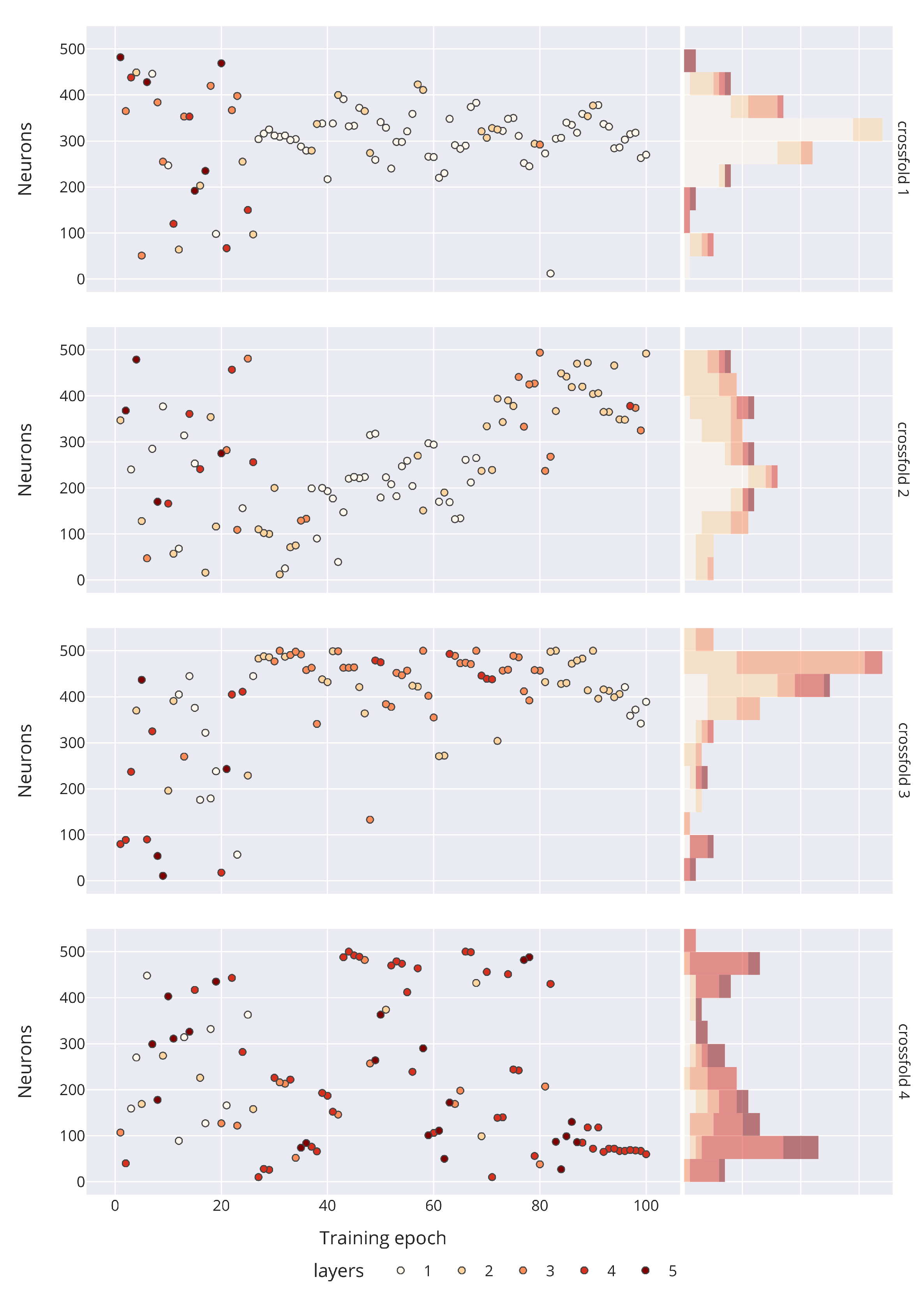
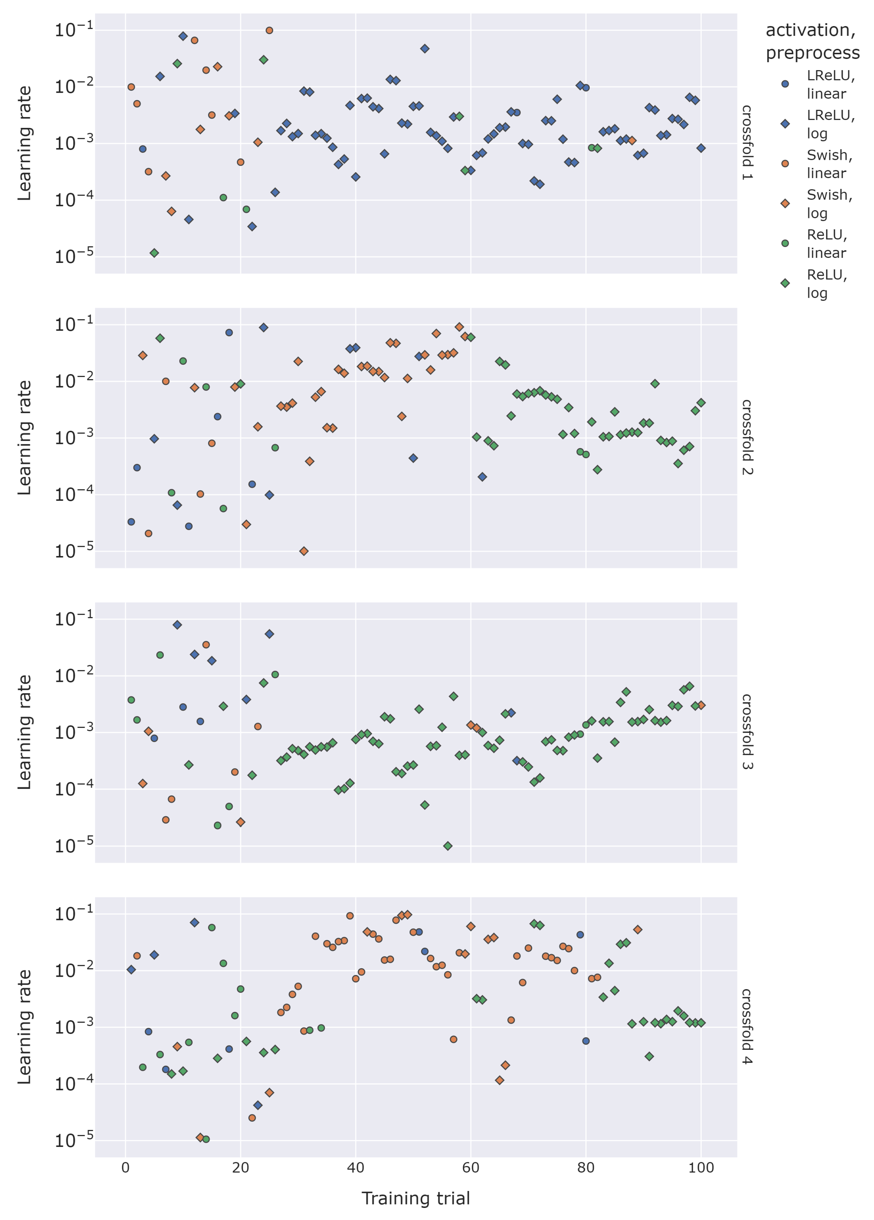
4.1. Model Architecture Exploration

The influence of the number of hidden layers on the performance of the network was investigated. The more layers, the higher fitting ability, possibly ending up in overfitting. A model with fewer layers runs faster; however, it lacks the same fitting capability. Therefore, networks having between one and five hidden layers were examined. The output layer for a binary classification problem should have one neuron with a sigmoid function, e.g., expressed by the logistic function.

The data normalization method, number of layers, number of neurons in each layer, learning rate, dropout rate, regularization rate, and activation function for the hidden layers were selected as the parameters forming the searched hyperspace. The choice of additional hyperparameters could allow for training a more efficient network, but it would involve an exponential increase of possible combinations. The selected parameters were considered to have a potentially significant contribution to the performance of the neural network.

The optimal number of layers was searched from the range $[1,5]$ and as an integer. Similarly, the number of neurons in each hidden layer was chosen. An integer number was picked uniformly from the range $[10,500]$, which was motivated by preserving speed, consuming low amount of memory, and maintaining the ability to generalise. Due to limitations of the algorithms used for searching the hyperparameter space, the number of neurons for each layer was generated once for all layers rather than separately for each one. This could potentially have an adverse effect on the results obtained.

Adam was selected as the optimization algorithm [27]. The parameters were set respectively: ${\beta }_1=0.9$, ${\beta }_2=0.999$, $ϵ={10}^{-7}$. The learning rate value was sampled from a lognormal distribution on the interval $[{10}^{-5},{10}^{-1}]$ and remained unchanged over the span of training epochs.

Dropout was implemented during training following each hidden layer. The dropout rate was drawn from a uniform distribution from interval $[0,0.5]$. The purpose of its implementation was maintaining the generalization ability of the network and comparing the effect of altering it with respect to the learning capability of the model.

The second type of used regularization involved adding a penalty to the total loss function. This was based on the ${\mathrm{L}}_2$ function (Equation (4)) applied to the weights of all neurons possessing them excluding the neuron in the last layer. The bias values were not affected by this function. The penalty factor was randomly drawn among the values $0.1$, $0.01$, $0.001$, $0.0001$, $0.00001$, 0, where the last value indicates that it was not applied. The reason for using a discrete variable instead of a continuous lognormal distribution was the inability to obtain zero to make the comparison of not involving ${\mathrm{L}}_2$ regularization.

The last examined hyperparameter was neuron activation function. By excluding the network output, it was applied identically to all neurons. Among the analysed functions were ReLU [25], LeakyReLU, and Swish [26]. In the case of LeakyReLU, whose coefficient $\alpha =0.2$, the purpose of the application was to compare whether it would perform better than ReLU. Swish is a relatively new activation function that in testing outperformed the other currently available solutions [26], so it was chosen as an alternative to the most widely applied activation functions.

4.2. Training Phase Setup

As a result of the unbalanced dataset, the random prediction prior to training would show poor performance by imputing equal likelihoods of belonging to either class. To counteract this, the bias of the last neuron in the network was initially set as:

$$b_{output}=ln\left(\frac{\mathrm{P}}{\mathrm{N}}\right)$$

(13)

where P is the number of positive samples in the training set, while N is the number of negative samples. Adjusting this value in this manner provides information to the network about unequal class sizes and helps avoid changing the bias to reach this value, thus speeding up training and reducing the value of the loss function in the initial steps.

The weights for all neurons in the network were initialised by the Glorot uniform initialiser [35] from range $[-l,l]$, where

$$l=\sqrt{\frac{6}{n_{in}+n_{out}}}$$

(14)

and $n_{in}$ is number of inputs connected to a given neuron, $n_{out}$ is number of output units. Biases were set to 0, with the exception of the output of the last layer.

Batch size is among the many factors that can affect the training of networks and consequently the performance achieved by them. The authors decided to set its size as 2048 as a compromise between training speed and maintaining generalization ability. The reason for not seeking the optimal value was caused by the large number of hyperparameters searched, as it would exponentially increase the possible combinations. Not searching the hyperparameter space thoroughly would have resulted in a larger difference between the best parameters obtained and their optimum values.

For the used dataset, the class sizes were unbalanced, which during training would adversely affect the less numerous P class denoting malicious traffic. Countermeasures against this include oversampling and assigning weights to the categories, which was applied. The calculated gradient was scaled in inverse proportion to the class numerosity in the training set.

Tune [36] is a unified framework which provides user and scheduler APIs for model training and selection. Implemented on top of the Ray [37] framework, it enables resource management and distributed execution. The optimization software Optuna [38] was selected to perform hyperparameter suggestion.

The tree-structured Parzen estimator (TPE) [39] algorithm was utilised to propose hyperparameters. It modifies the prior distributions to enhance the likelihood of locating the optimal values of the specified hyperparameters. The probability distributions are modified accordingly: uniform to truncated Gaussian mixture, log-uniform to exponentiated truncated Gaussian mixture, categorical to re-weighted categorical. Before launching the TPE algorithm, a random search was applied in the first 25 runs to provide a broader search of the available hyperspace before modifying the distributions.

In contrast to model training, which may have various goals (e.g., maximizing accuracy) but for most types of networks relies on minimizing the loss function, the objective and way of optimizing hyperparameters could be identical. Optuna allows the user to choose any metric to be the objective function to minimise or maximise. In the case of this paper, the decision was made to choose the metric ${\mathrm{F}}_2$ score given by Section 2.2 and maximise it. Due to the unbalanced set, accuracy would not be a suitable metric, while ${\mathrm{F}}_2$ score takes into consideration precision and recall, which describe such sets better. The use of $\beta =2$ in the ${\mathrm{F}}_{\beta }$ score is intended to give more weight to recall, which reflects the higher importance of ignoring malicious traffic than precision, which represents the misclassification of benign traffic.

Another additional optimization algorithm utilised was ASHA [40], which was implemented in Tune. It assists in searching by limiting resources for less promising trials. In practice, this means stopping training for an unpromising set of hyperparameters and proceeding to the next one suggested by the sampler. As with TPE, the objective function was the ${\mathrm{F}}_2$ score, which was maximised. Training iteration, or epoch, was set as the time attribute. The maximum training time was set to 25 epochs, the grace period denoting the minimum number of training iterations after which ASHA may declare the hyperparameters unpromising and stop training was set to 1. The reduction factor $\eta$ defining the number of steps after which approximately $1/\eta$ of runs shall remain and increasing their budget by $\eta$, which, upon reaching, rescreening will occur again, was set to 3.

Training was performed on four crossfolds from a subset designated for training and validation. Each time, 100 configurations were tested, the last 75 of which were suggested by the TPE algorithm on the basis of previously achieved ${\mathrm{F}}_2$ score values. This yielded 400 configurations.

For each crossfold, five configurations were selected for which the largest ${\mathrm{F}}_2$ score values were obtained on the corresponding validation set. Twenty new models were created and trained on the complete subset designated for training and validation. Normalization was applied using the new set. A test set representing 20% of the entire dataset was used as a validation subset. The purpose of this procedure was to exclude differences caused by how the original set was divided. Each time, the training lasted 25 epochs and was done without additional interference.

5. Results

The detailed results for the top five achieved values of ${\mathrm{F}}_2$ on the validation set for each crossfold are shown in

Table 2. The best five results for each crossfold (the highest values are underlined).

Id/ Crossfold	Train. Accuracy	Train. Recall	Train. Precision	Train. ${\mathbf{F}}_2$	Valid. Accuracy	Valid. Recall	Valid. Precision	Valid. ${\mathbf{F}}_2$
1/1	0.985279	0.953011	0.952642	0.952938	0.985035	0.953709	0.952691	0.953505
2/1	0.985187	0.952982	0.952175	0.952821	0.985194	0.953672	0.950938	0.953124
3/1	0.984720	0.951857	0.949798	0.951445	0.984740	0.953398	0.951399	0.952997
4/1	0.984624	0.951583	0.949958	0.951257	0.984706	0.953201	0.951103	0.952781
5/1	0.984882	0.952582	0.951060	0.952277	0.984641	0.953459	0.950000	0.952765
6/2	0.985692	0.953451	0.956237	0.954007	0.985788	0.954082	0.959513	0.955164
7/2	0.984982	0.952545	0.950739	0.952183	0.985490	0.953705	0.959159	0.954791
8/2	0.985753	0.953149	0.957078	0.953932	0.985614	0.954214	0.957105	0.954790
9/2	0.985165	0.952379	0.952324	0.952368	0.985624	0.953886	0.957250	0.954557
10/2	0.985511	0.953122	0.955194	0.953535	0.985433	0.954117	0.956280	0.954549
11/3	0.985379	0.953305	0.952827	0.953210	0.985560	0.953694	0.961175	0.955181
12/3	0.985684	0.953531	0.955238	0.953872	0.985958	0.953829	0.960620	0.955179
13/3	0.985661	0.953270	0.955329	0.953681	0.985936	0.953439	0.961442	0.955029
14/3	0.985669	0.953469	0.955617	0.953898	0.986002	0.953506	0.961032	0.955002
15/3	0.985751	0.953546	0.955750	0.953986	0.985892	0.953739	0.960023	0.954990
16/4	0.984692	0.951712	0.950179	0.951405	0.985614	0.953164	0.954426	0.953416
17/4	0.984678	0.952081	0.949842	0.951632	0.985164	0.953404	0.952390	0.953201
18/4	0.984547	0.951736	0.948676	0.951123	0.984852	0.953241	0.952025	0.952997
19/4	0.984425	0.951777	0.948229	0.951065	0.984818	0.953062	0.951772	0.952804
20/4	0.984702	0.952451	0.949359	0.951831	0.984788	0.953401	0.950232	0.952765

. The differences in the achieved metrics computed from identical sets vary on the thousandths position, which may suggest a proximity to a local or global maximum for the hyperparameter space. The differences between the crossfolds may be caused by the different difficulties of the validation sets or by the achieving selection of different probability distributions corresponding to different local maxima by the TPE algorithm.

A comparison of the performance of the metrics during the last training epoch on the training set and the validation set for the top 20 values of ${\mathrm{F}}_2$ achieved on the validation set is shown in Figure 2. As expected, the accuracy reaches the highest value, which is caused by the unbalanced set. In most instances, for each metric, the value is higher on the validation set, which should not happen since training, i.e., fitting the network to the dataset, is performed on the training set. The explanation behind this is dropout, which is only present during training. It helps to preserve generalization ability, which comes at the cost of reduced ability to fit the training set. Eliminating the dropout after training eliminates this problem. It likewise would allow for better performance on the training set.

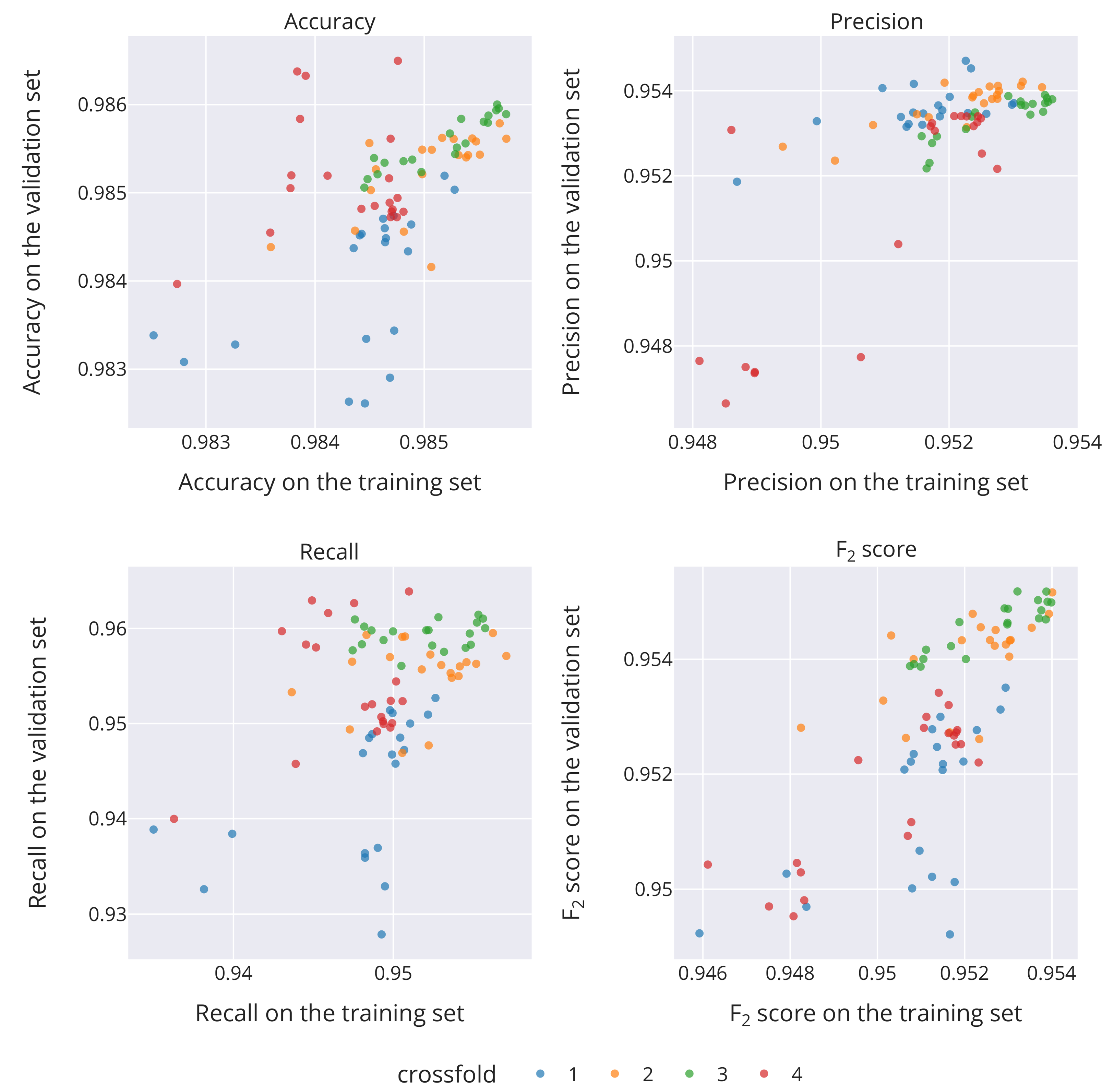
5.1. Analysis of Crossfolds

Hyperparameters in the models during each crossfold were generated independently. Every time after the first 25 random iterations, the TPE algorithm analysed the results and changed the probability distributions of the variables. During the remaining 75 iterations, the algorithm parameters continued to evolve incorporating the new results. The hyperparameter values for the best five ${\mathrm{F}}_2$ score values were obtained on the validation set and are shown in

Table 3. The best five configurations for each crossfold (all models used logarithmic normalization).

Id/ Crossfold	Layers	Neurons	Activation	Learing Rate	${\mathbf{L}}_2$ reg.	Dropout	Train. ${\mathbf{L}}_2$	Valid. ${\mathbf{L}}_2$
1/1	1	332	LReLU	$4.147\times {10}^3$	0	0.001494	0.952938	0.953505
2/1	1	312	LReLU	$1.499\times {10}^{-3}$	0	0.004133	0.952821	0.953124
3/1	1	338	LReLU	$4.708\times {10}^{-3}$	0	0.035715	0.951445	0.952997
4/1	2	321	LReLU	$1.000\times {10}^{-3}$	${10}^{-5}$	0.016339	0.951257	0.952781
5/1	1	325	LReLU	$1.325\times {10}^{-3}$	${10}^{-5}$	0.002084	0.952277	0.952765
6/2	2	237	ReLU	$5.391\times {10}^{-3}$	0	0.003140	0.954007	0.955164
7/2	2	367	ReLU	$1.049\times {10}^{-3}$	${10}^{-5}$	0.078722	0.952183	0.954791
8/2	1	265	ReLU	$5.977\times {10}^{-3}$	0	0.000635	0.953932	0.954790
9/2	2	419	ReLU	$1.145\times {10}^{-3}$	${10}^{-5}$	0.050924	0.952368	0.954557
10/2	1	261	ReLU	$1.952\times {10}^{-2}$	0	0.001476	0.953535	0.954549
11/3	2	414	ReLU	$1.559\times {10}^{-3}$	0	0.108125	0.953210	0.955181
12/3	2	396	ReLU	$2.535\times {10}^{-3}$	0	0.030578	0.953872	0.955179
13/3	1	421	ReLU	$2.892\times {10}^{-3}$	0	0.049736	0.953681	0.955029
14/3	1	342	ReLU	$2.941\times {10}^{-3}$	0	0.024507	0.953898	0.955002
15/3	2	500	ReLU	$1.696\times {10}^{-3}$	0	0.031615	0.953986	0.954990
16/4	4	67	ReLU	$1.943\times {10}^{-3}$	${10}^{-5}$	0.005776	0.951405	0.953416
17/4	4	85	ReLU	$1.149\times {10}^{-3}$	${10}^{-5}$	0.015252	0.951632	0.953201
18/4	1	166	ReLU	$5.624\times {10}^{-4}$	${10}^{-5}$	0.163120	0.951123	0.952997
19/4	4	67	ReLU	$1.194\times {10}^{-3}$	${10}^{-5}$	0.014062	0.951065	0.952804
20/4	4	65	ReLU	$1.202\times {10}^{-3}$	${10}^{-5}$	0.002810	0.951831	0.952765

.

Both similarities and differences are noticeable among the models, often a different value appears during a distinct crossfold. The applied algorithms did not guarantee that optimal (in this case maximum) values would be found. Most probably, different local maxima were found, which is caused by various numbers drawn by the pseudorandom generators as well as differences between the datasets.

The number of layers in the most effective models is relatively low. The change in its value along with the number of neurons in each of them over train trials is presented in Figure 3. During the first 25 iterations, parameters were generated from uniform distributions, after which subsequent suggestions were determined by the TPE algorithm. If the results for higher numbers of layers were not good, subsequent selection was less likely. This situation is particularly evident in the first crossfold. The inverse of this is the fourth crossfold in which greater weights were given to higher numbers of layers. In both cases, no conversion took place, making it impossible to draw clear conclusions about the optimal number of layers given the similar results.

The number of neurons in each layer showed more variation. In the second crossfold, better values were obtained by increasing the number of neurons. Determining the optimal number of them is not possible, but, for most models, increasing their number brings improvement. An exception can be observed in crossfold no. 4, which may be caused by the larger number of layers used. From the combination of these influences, the model could overfit.

Learning rates, activation functions, and methods of preprocessing selected during trials were presented in Figure 4. The absence of Swish activation functions among the most accurate models must have been caused by its lesser suitability to the classification problem being undertaken. In crossfolds no. 2 and no. 4, it was superseded by ReLU. The latter cannot be unequivocally considered superior to LReLU, although it was more frequently selected.

The consistent use of normalization with prior logarithmic transformation is supported by the graphs. Only in case 4 of the crossfold linear normalization performed better until more tests involving logarithmic were conducted. This clear result confirms the increase in performance achievable by attempting to converge the initial distribution of features to a uniform one.

Learning rate is one of the hyperparameters purely responsible for training. The Adam optimization algorithm was used for each model, and the only difference within it was the change in learning rate $\alpha$. This permits a more meaningful comparison of the learning rate parameter, since among the hyperparameters searched, only the number of layers had a large effect on it. In each case, the best values were found in the range $[0.001,0.01]$, despite attempts to search a wider interval. Since throughout training the learning rate was constant and the change in gradient was modified only by the Adam algorithm, this value was forced to become the highest that provides effective training. Lower values, despite the ability to learn the network, were eliminated by the ASHA algorithm stopping unpromising trials, i.e., those that do not achieve high enough performance quickly.

The evolution of hyperparameters that directly influence against overfitting is shown in Figure 5. In the case of ${\mathrm{L}}_2$ regularization rate, lower values were most frequently adopted: ${10}^{-5}$ and 0. A potential explanation is the inability to accurately match the training set, which may have been caused by the limited capabilities of the network. Another factor that may have contributed to these results may have been the similarity of the training and validation sets. Regularization slows down the matching and therefore the ASHA algorithm may have also terminated trials prematurely. Even during later trials, large values of ${\mathrm{L}}_2$ regularization rate were tested. The logarithmic uniform distribution was replaced by a categorical one with weights, in order to be able to underutilise the regularization by setting its value to 0. The probability weights were adjusted separately for each value, which resulted in larger values also appearing in later trials.

Dropout rates, similarly to ${\mathrm{L}}_2$ regularization, eventually take on lower values. Higher values were also tested in each crossfold, but ultimately remained lower than $0.1$. As with regularization, the cause may lie in similarity of sets, low network capacity, or premature termination by the ASHA algorithm. The values became low but remained clearly above zero, which may suggest the usefulness of dropout.

5.2. Complete Dataset

To decouple the results from variations in the samples contained in each crossfold, the networks were re-trained for the top five sets of hyperparameters for each crossfold. The training set consisted of the entire subset used to search the hyperparameter space while the validation set constituted the test subset, which until now had not been used by any of the models. The achieved results are shown in

Table 4. Results of best model configurations on a complete dataset (the highest values are underlined).

Id	Train. Accuracy	Train. Recall	Train. Precision	Train. ${\mathbf{F}}_2$	Valid. Accuracy	Valid. Recall	Valid. Precision	Valid. ${\mathbf{F}}_2$
1	0.985487	0.953338	0.953400	0.953351	0.985623	0.954242	0.960193	0.955426
2	0.985770	0.953545	0.955593	0.953954	0.986016	0.954449	0.959681	0.955491
3	0.985740	0.953497	0.956524	0.954101	0.985968	0.953800	0.959513	0.954937
4	0.985785	0.953557	0.956156	0.954075	0.985951	0.954351	0.959907	0.955457
5	0.985790	0.953463	0.956371	0.954043	0.986057	0.953903	0.961583	0.955430
6	0.985799	0.953694	0.955807	0.954116	0.985986	0.954495	0.958517	0.955297
7	0.985114	0.952619	0.951175	0.952330	0.985563	0.952987	0.960972	0.954573
8	0.985877	0.953384	0.958321	0.954367	0.985748	0.954353	0.959537	0.955385
9	0.985319	0.952743	0.952580	0.952711	0.985581	0.953927	0.958010	0.954741
10	0.985503	0.953170	0.955167	0.953569	0.985391	0.954318	0.956221	0.954698
11	0.985487	0.953093	0.953714	0.953217	0.985589	0.954371	0.955108	0.954518
12	0.984550	0.951748	0.949164	0.951230	0.984963	0.953843	0.950701	0.953213
13	0.984738	0.951941	0.949854	0.951523	0.985582	0.953640	0.953506	0.953613
14	0.985280	0.953007	0.952763	0.952959	0.985375	0.954340	0.953199	0.954112
15	0.984895	0.952168	0.950591	0.951852	0.985389	0.953303	0.960285	0.954691
16	0.984724	0.951835	0.950323	0.951532	0.984730	0.954145	0.949748	0.953263
17	0.984427	0.951339	0.948442	0.950758	0.984880	0.953596	0.953865	0.953650
18	0.984565	0.951510	0.949802	0.951168	0.984657	0.954147	0.947953	0.952902
19	0.984889	0.952499	0.951215	0.952242	0.984685	0.954169	0.949517	0.953235
20	0.984774	0.952610	0.949929	0.952073	0.985427	0.954007	0.952854	0.953776

. The values in the id column correspond to those in Table 3.

The new results were slightly better than those achieved on a fraction of the dataset, which may be due to increasing the training set from 60 to 80 percent of the total available samples while keeping the validation set at 20 percent. This also implies that the dataset was properly shuffled before splitting. The ranking order of the best hyperparameters changed slightly, which could have been caused by changing the datasets or initialization of the weights. The best ${\mathrm{F}}_2$ score value was achieved by model 2 and reached $0.955491$.

6. Discussion

The models with high performance in detecting various network attacks were trained. However, the performance for each type of attack was also examined (for the best model). The chosen binary classification approach allowed only the detection of malicious traffic without specifying its category. It is worth discussing effectiveness in the detection of each type of attack in order to compare different types and determine which type characterises the highest detection ratios.

During the analysis, the authors find that the achieved performance for most attacks was very high. False alarms occurred in about 0.8% cases, but model development based on the ${\mathrm{F}}_2$ score metric was more focused on attack detection. Lower performance was achieved for Infiltration, Brute Force-Web, Brute Force-XSS, and SQL Injection attacks. In the case of the first of these, the reason may have been the similarity of the traffic generated by the compromised host to other users, which may have significantly hindered detection. The remaining attacks also do not have characteristic features that distinguish them from benign traffic. However, treating all types of traffic equally could be considered as the main reason, and because of the smaller number of samples, the performance achieved on them would be lower, as it was more profitable for the network in terms of loss function to match more numerous classes. Countermeasures could have been oversampling or increasing the weight for samples from less numerous attacks.

7. Conclusions

Security in cyberspace is a major challenge of modern IT systems, including smart grids. Most of the attacks are performed by leveraging the communication channel to gain unauthorised access or disrupt services. This paper presents a method for detecting attacks by analysing network traffic using traffic flow statistical analysis, which works on encrypted traffic. The results indicate very high effectiveness; however, this is a heuristic-based method—thus it does not provide complete guarantee of detection. Therefore, it should be used in conjunction with other techniques, e.g., signature-based attack detection approach.

The paper described the principles of a heuristic algorithm based on a neural network. The used dataset was presented, including details related to data processing and needed modifications before machine learning step. The process of learning the artificial neural networks and fine-tuning its hyperparameters was demonstrated. The final results proved the high effectiveness and precision of this approach—the models achieved accuracy higher than 98% and ${\mathrm{F}}_2$ score higher than 95%. It allows for very effective intrusion detection in practice.

Future research can be focused on setting of neural network hyperparameters aiming for improved results. There is also a possibility to test the applied methodology on a new dataset and implement the solution in a practical network environment to verify heuristic detection in real-time scenarios. Additionally, an attempt to obtain similar performance indexes while reducing the number of features of each flow could be made.

References

1. Tufail, S.; Parvez, I.; Batool, S.; Sarwat, A. A Survey on Cybersecurity Challenges, Detection, and Mitigation Techniques for the Smart Grid. Energies 2021, 14, 5894. [Google Scholar] [CrossRef]
2. Liang, G.; Zhao, J.; Luo, F.; Weller, S.R.; Dong, Z.Y. A Review of False Data Injection Attacks Against Modern Power Systems. IEEE Trans. Smart Grid 2017, 8, 1630–1638. [Google Scholar] [CrossRef]
3. Alghassab, M. Analyzing the Impact of Cybersecurity on Monitoring and Control Systems in the Energy Sector. Energies 2022, 15, 218. [Google Scholar] [CrossRef]
4. Nait Belaid, Y.; Coudray, P.; Sanchez-Torres, J.; Fang, Y.P.; Zeng, Z.; Barros, A. Resilience Quantification of Smart Distribution Networks—A Bird’s Eye View Perspective. Energies 2021, 14, 2888. [Google Scholar] [CrossRef]
5. Liu, X.; Song, Y.; Li, Z. Dummy Data Attacks in Power Systems. IEEE Trans. Smart Grid 2020, 11, 1792–1795. [Google Scholar] [CrossRef]
6. Al-Asli, M.; Ghaleb, T.A. Review of Signature-based Techniques in Antivirus Products. In Proceedings of the 2019 International Conference on Computer and Information Sciences (ICCIS), Sakaka, Saudi Arabia, 3–4 April 2019; pp. 1–6. [Google Scholar]
7. Samrin, R.; Vasumathi, D. Review on anomaly based network intrusion detection system. In Proceedings of the 2017 International Conference on Electrical, Electronics, Communication, Computer, and Optimization Techniques (ICEECCOT), Mysuru, India, 15–16 December 2017. [Google Scholar]
8. Sun, C.C.; Sebastian Cardenas, D.J.; Hahn, A.; Liu, C.C. Intrusion Detection for Cybersecurity of Smart Meters. IEEE Trans. Smart Grid 2021, 12, 612–622. [Google Scholar] [CrossRef]
9. Musleh, A.S.; Chen, G.; Dong, Z.Y. A Survey on the Detection Algorithms for False Data Injection Attacks in Smart Grids. IEEE Trans. Smart Grid 2020, 11, 2218–2234. [Google Scholar] [CrossRef]
10. Karimipour, H.; Dehghantanha, A.; Parizi, R.M.; Choo, K.K.R.; Leung, H. A Deep and Scalable Unsupervised Machine Learning System for Cyber-Attack Detection in Large-Scale Smart Grids. IEEE Access 2019, 7, 80778. [Google Scholar] [CrossRef]
11. Dini, P.; Saponara, S. Analysis, Design, and Comparison of Machine-Learning Techniques for Networking Intrusion Detection. Designs 2021, 5, 9. [Google Scholar] [CrossRef]
12. Kao, M.T.; Sung, D.Y.; Kao, S.J.; Chang, F.M. A Novel Two-Stage Deep Learning Structure for Network Flow Anomaly Detection. Electronics 2022, 11, 1531. [Google Scholar] [CrossRef]
13. Ullah, S.; Khan, M.A.; Ahmad, J.; Jamal, S.S.; e Huma, Z.; Hassan, M.T.; Pitropakis, N.; Arshad; Buchanan, W.J. HDL-IDS: A Hybrid Deep Learning Architecture for Intrusion Detection in the Internet of Vehicles. Sensors 2022, 22, 1340. [Google Scholar] [CrossRef] [PubMed]
14. Almaraz-Rivera, J.G.; Perez-Diaz, J.A.; Cantoral-Ceballos, J.A. Transport and Application Layer DDoS Attacks Detection to IoT Devices by Using Machine Learning and Deep Learning Models. Sensors 2022, 22, 3367. [Google Scholar] [CrossRef]
15. Le, K.H.; Nguyen, M.H.; Tran, T.D.; Tran, N.D. IMIDS: An Intelligent Intrusion Detection System against Cyber Threats in IoT. Electronics 2022, 11, 524. [Google Scholar] [CrossRef]
16. Kurt, M.N.; Ogundijo, O.; Li, C.; Wang, X. Online Cyber-Attack Detection in Smart Grid: AReinforcement Learning Approach. IEEE Trans. Smart Grid 2019, 10, 5174–5185. [Google Scholar] [CrossRef] [Green Version]
17. Boyaci, O.; Narimani, M.R.; Davis, K.R.; Ismail, M.; Overbye, T.J.; Serpedin, E. Joint Detection and Localization of Stealth False Data Injection Attacks in Smart Grids Using Graph Neural Networks. IEEE Trans. Smart Grid 2022, 13, 807–819. [Google Scholar] [CrossRef]
18. He, Y.; Mendis, G.J.; Wei, J. Real-Time Detection of False Data Injection Attacks in Smart Grid: A Deep Learning-Based Intelligent Mechanism. IEEE Trans. Smart Grid 2017, 8, 2505–2516. [Google Scholar] [CrossRef]
19. Singer, P.W.P.W. Cybersecurity and Cyberwar: What Everyone Needs to Know; Oxford University Press: Cary, NC, USA, 2014. [Google Scholar]
20. Smolarczyk, M.; Plamowski, S.; Pawluk, J.; Szczypiorski, K. Anomaly Detection in Cyclic Communication in OT Protocols. Energies 2022, 15, 1517. [Google Scholar] [CrossRef]
21. Mittal, M.; de Prado, R.P.; Kawai, Y.; Nakajima, S.; Muñoz-Expósito, J.E. Machine Learning Techniques for Energy Efficiency and Anomaly Detection in Hybrid Wireless Sensor Networks. Energies 2021, 14, 3125. [Google Scholar] [CrossRef]
22. Niemiec, M.; Kościej, R.; Gdowski, B. Multivariable Heuristic Approach to Intrusion Detection in Network Environments. Entropy 2021, 23, 776. [Google Scholar] [CrossRef] [PubMed]
23. Shaukat, K.; Luo, S.; Varadharajan, V.; Hameed, I.A.; Chen, S.; Liu, D.; Li, J. Performance Comparison and Current Challenges of Using Machine Learning Techniques in Cybersecurity. Energies 2020, 13, 2509. [Google Scholar] [CrossRef]
24. Goodfellow, I.; Bengio, Y.; Courville, A. Deep Learning; MIT Press: Cambridge, MA, USA, 2016. [Google Scholar]
25. Arora, R.; Basu, A.; Mianjy, P.; Mukherjee, A. Understanding Deep Neural Networks with Rectified Linear Units. arXiv 2016, arXiv:1611.01491. [Google Scholar] [CrossRef]
26. Ramachandran, P.; Zoph, B.; Le, Q.V. Searching for Activation Functions. arXiv 2017, arXiv:1710.05941. [Google Scholar]
27. Kingma, D.P.; Ba, J. Adam: A method for stochastic optimization. arXiv 2014, arXiv:1412.6980. [Google Scholar]
28. Tieleman, T.; Hinton, G. Lecture 6.5-rmsprop: Divide the gradient by a running average of its recent magnitude. Neural Netw. Mach. Learn. 2012, 4, 26–31. [Google Scholar]
29. Duchi, J.; Hazan, E.; Singer, Y. Adaptive subgradient methods for online learning and stochastic optimization. J. Mach. Learn. Res. 2011, 12, 2121–2159. [Google Scholar]
30. Cortes, C.; Mohri, M.; Rostamizadeh, A. L2 Regularization for Learning Kernels. In Proceedings of the Twenty-Fifth Conference on Uncertainty in Artificial Intelligence, Montreal, QC, Canada, 18–21 June 2009; AUAI Press: Arlington, VI, USA, 2009; pp. 109–116. [Google Scholar]
31. Hinton, G.E.; Srivastava, N.; Krizhevsky, A.; Sutskever, I.; Salakhutdinov, R.R. Improving neural networks by preventing co-adaptation of feature detectors. arXiv 2012, arXiv:1207.0580. [Google Scholar]
32. Sharafaldin, I.; Lashkari, A.H.; Ghorbani, A.A. Toward generating a new intrusion detection dataset and intrusion traffic characterization. ICISSP 2018, 1, 108–116. [Google Scholar] [CrossRef]
33. CICFlowMeter. Available online: https://www.unb.ca/cic/research/applications.html#CICFlowMeter (accessed on 16 May 2022).
34. A Realistic Cyber Defense Dataset (CSE-CIC-IDS2018). Available online: https://registry.opendata.aws/cse-cic-ids2018/ (accessed on 16 May 2022).
35. Glorot, X.; Bengio, Y. Understanding the difficulty of training deep feedforward neural networks. In Proceedings of the 13th International Conference on Artificial Intelligence and Statistics, Sardinia, Italy, 13–15 May 2010; JMLR Workshop and Conference Proceedings. pp. 249–256. [Google Scholar]
36. Liaw, R.; Liang, E.; Nishihara, R.; Moritz, P.; Gonzalez, J.E.; Stoica, I. Tune: A Research Platform for Distributed Model Selection and Training. arXiv 2018, arXiv:1807.05118. [Google Scholar]
37. Moritz, P.; Nishihara, R.; Wang, S.; Tumanov, A.; Liaw, R.; Liang, E.; Elibol, M.; Yang, Z.; Paul, W.; Jordan, M.I.; et al. Ray: A Distributed Framework for Emerging AI Applications. In Proceedings of the 13th USENIX Symposium on Operating Systems Design and Implementation (OSDI 18), Carlsbad, CA, USA, 8–10 October 2018; pp. 561–577. [Google Scholar]
38. Akiba, T.; Sano, S.; Yanase, T.; Ohta, T.; Koyama, M. Optuna: A Next,-generation Hyperparameter Optimization Framework. In Proceedings of the 25rd ACM SIGKDD International Conference on Knowledge Discovery and Data Mining, Anchorage, AK, USA, 4–8 August 2019. [Google Scholar]
39. Bergstra, J.; Bardenet, R.; Bengio, Y.; Kégl, B. Algorithms for hyper-parameter optimization. In Advances in Neural Information Processing Systems; Curran Associates, Inc.: Red Hook, NY, USA, 2011; Volume 24. [Google Scholar]
40. Li, L.; Jamieson, K.; Rostamizadeh, A.; Gonina, E.; Hardt, M.; Recht, B.; Talwalkar, A. A System for Massively Parallel Hyperparameter Tuning. arXiv 2020, arXiv:1810.05934. [Google Scholar]
Figure 1. Histograms of selected numeric features in logarithmic scale for a complete dataset.
Energies 15 03951 g001
Figure 2. Metrics during the last epoch of training and validation—top 20 results for each crossfold.
Energies 15 03951 g002
Figure 3. Changes in number of layers and neurons during trials for each crossfold.
Energies 15 03951 g003
Figure 4. Changes in learning rate, activation function, and preprocessing method during trials for each crossfold.
Energies 15 03951 g004
Figure 5. Changes in dropout and L 2 regularization rate during trials for each crossfold.
Energies 15 03951 g005